A recursive model of residual life prediction for human beings with health information from activities of daily living and memory

Abstract

As the ageing population increases, it is essential to manage human resources with residual life prediction, especially for the ageing population. Thus, this study aims to predict residual life using the available information of health statuses, such as the performances in activities of daily living (ADL) and memory. In this study, the principal components of ADL and memory information are extracted for prediction. The relationship between the principal components and residual life is established based on the concept of the proportional residual, which states that the residual life may be proportional to the changes in ADL and memory performance. A recursive model for residual life prediction is formulated and fitted for the Chinese Health and Nutrition Survey data. Finally, a goodness-of-fit test is conducted, and an example case is presented. The results show that the fitted model in this study is more accurate and precise than the original, unfitted model to estimate the residual life of human beings. This study is advantageous over existing studies in two aspects: (1) the model is formulated using a recursive method based on stochastic filtering; (2) the data include both physical status and mental status.

KEYWORDS:

• Stochastic filtering
• recursive model
• health information
• activities of daily living
• memory

1. Introduction

Currently, live expectancy surpasses the age of 60 (de Cabo & Mattason, 2019; DESA, 2007; Fitzmaurice et al., 2019; Rudd et al., 2020; Word Health Organization, 2015). This demographic brings unprecedented opportunities and challenges. Longer life can be an incredibly valuable resource in economic, social, cultural, and familial aspects (Beard & Bloom, 2015). However, the healthcare expenditures for older people are increasing over time (Gregersen, 2014). The increasing prevalence of chronic diseases associated with ageing that accompanies the growth of the elderly population makes it hard for health and care services to cope (Oliver et al., 2014). Previous research shows that the expected cumulative expenditures for healthier elderly persons are similar to those of less healthy individuals (Lubitz et al., 2003). This implies that if we can estimate the health status of the aged person, their possible expenditure in a good health condition can be saved. Intuitively, a direct reflection of health status is the residual life. Thus, if a healthcare system wants to manage health better and reduce costs, an effective residual life prediction is needed.

Many researchers have studied life prediction for human beings using life expectancy or mortality (Arora et al., 2016; Atance et al., 2020; Boudoulas et al., 2017; Evans & Soliman, 2019; Parker et al., 2020; Wandeler et al., 2016; Wang et al., 2018). Traditional studies investigated this topic from the perspective of disease. Wandeler et al. studied the trends in life expectancy of HIV-positive adults on antiretroviral therapy worldwide (Wandeler et al., 2016). Wang et al. proposed a mortality prediction system for heart failure with orthogonal relief and dynamic radius means (Wang et al., 2018). Another stream of studies investigated this topic from the perspective of non-disease factors. For instance, Boudoulas et al. reviewed the effect of the evolution of medical science and medical technology on life expectancy (Boudoulas et al., 2017). Evans and Soliman presented an ecological study on the relationship between the subjective sense of well-being and life expectancy (Evans & Soliman, 2019). Parker et al. provided a systematic review on healthy working life expectancy at age 50 (Parker et al., 2020).

Besides traditional statistical studies, some researchers tried to study life expectancy or mortality using mathematical models (Hashir & Sawhney, 2020; Li et al., 2017; Su et al., 2020). For example, Li et al. used machine learning models to predict in-hospital mortality of ST-elevation myocardial infarction patients (Li et al., 2017). Su et al. developed a clinical prediction model for the mortality of diabetic adults with COVID-19 in Wuhan, China (Su et al., 2020). Hashir and Sawhney attempted to predict mortality with free-text clinical notes (Hashir & Sawhney, 2020). However, these mathematical models are limited to a population with a specific disease, while healthcare requires a comprehensive health assessment or residual life prediction for an average person. Some researchers developed models to estimate age-specific mortality for an average person (Cho et al., 2020). For instance, Cho et al. proposed an age-structured biomass model with an impulsive dynamic system to estimate age-specific natural mortality (Cho et al., 2020), Díaz-Rojo et al. used a multivariate control chart and Lee-Carter models to study mortality changes (Díaz-Rojo et al., 2020).

However, both streams of studies have limitations. On the one hand, these traditional studies were carried out with statistical approaches, lacking the support of the change mechanism for life prediction and the results of quantitative analysis cannot be interpreted clearly (Atance et al., 2020). These studies cannot be easily used to guide healthcare workers, especially when they want to implement the healthcare policy to older adults, since these studies cannot explain the life prediction mechanism. These mathematical models of age-specific mortality did not utilize other health information except age, reducing the prediction accuracy. For example, aged people with better health status than age match groups may live longer than expected. Herein, it is recommended to utilize health information to adjust the residual life prediction.

Thus, this study proposes a recursive model to estimate the residual life of human beings with the utilization of health information to obtain a comprehensive health assessment (Senne, 1972). This estimation is related to the recursive filtering problem (Liu et al., 2021; Yang et al., 2021). Herein, the proposed model is constructed based on a stochastic filtering model, which was initially proposed by Wang and Christer (2000) for condition-based monitoring maintenance applications and then applied in life prediction for machines with vibration monitoring (Wang et al., 2018). This model is essentially a recursive Bayesian algorithm that is advanced in two aspects. First, it can track the subject’s progress and thus predict the outcome without information loss. Second, since the information is fully utilized, the prediction is more accurate and precise. Thus, this method can provide an effective view of the health status observed over one’s lifetime to estimate the residual life for human beings.

Moreover, this study also makes innovation in terms of information utilized. The previous research works of residual life prediction for the elderly are usually based only on the physiological conditions of the elderly, ignoring the influence of mental factors. To provide a more accurate prediction of the remaining life of the elderly, mental factors, such as the performance in memory, were introduced within the physical health indicators, such as the performance in Activities in Daily Life (ADL) in this study. In other words, the filtering approach is adapted to use both disability and cognitive impairment information, which have been proved to associate closely with later life loss (Jagger et al., 2007; Spiers et al., 2005; Stuck et al., 1999). The level of disability can be reflected by the performance in ADL (Covinsky et al., 2003; Dunlop et al., 1997; Katz, 1983), while the decline of cognitive function can be reflected by the memory impairment (Brewer et al., 2005; McGuire et al., 2006). Therefore, ADL and memory performance changes can be used as early indicators of mortality risk to estimate the residual life.

People may question why medical history, especially related to severe diseases, is not employed to predict the residual life in this study. For this issue, this study has four concerns. First, the medical history is not easily collected since people may be reluctant to talk about this sensitive topic. Second, only a fraction of people have access to their medical history, so that the application of the method utilizing medical history is limited. Third, medical history information is also difficult to be unified because patients are treated in different medical institutions or doctors with different treatment plans. Last, the medical history cannot reflect some sub-health status conditions without the diagnosis of disease, and these sub-health status conditions may also cause a reduction of residual life.

The remainder of this paper is arranged as follows. Section 2 presents the introduction and the initial process of data and variables used. Section 3 gives the model formulation process. Section 4 fits the proposed model according to the Chinese Health and Nutrition Survey (CHNS) data, a nationally representative survey in China. Section 5 provides a case study to illustrate the proposed model. Section 6 discusses, and Section 7 concludes this study, respectively.

2. Data and variables

This study uses longitudinal data from the Chinese Health and Nutrition Survey (CHNS) conducted by the Carolina Population Centre at the University of North Carolina at Chapel Hill, U.S.A., and the National Institute of Nutrition and Food Safety at the Chinese Centre for Disease Control and Prevention. CHNS started in 1989, and there were eight follow-up surveys between 1991 and 2011. CHNS used a multi-stage, random cluster method to draw samples from 19,000 participants from 4400 households in nine provinces, which made these samples substantially varied in geography, economic development, public resources, and health indicators (Popkin et al., 2009).

The general retirement age in China is around 55; thus, the ADL and memory tests are designed for adults aged 55 and older in the CHNS questionnaire. Therefore, the elderly is defined as adults older than 55 years old when their follow-up began, and in this study, all the analyses were performed for this population only. Excluding participants with invalid, erroneous, and incomplete cases on variables of concern, the total number of samples in our analyses is 10,986. Among them, 1746 samples recorded the age of death (complete), while the other samples are still alive at the last survey (censored), as shown in Table 1.

Table 1. Sample statistics.

		Life	Age at the first survey	Survey times
Type	Number	Mean (Median)
Complete	1746	74.3 (75)	66.05 (64.36)	2.536 (3)
Censored	9240		61.40 (59.01)	2.643 (3)
Total	10,986		62.14 (59.74)	2.626 (3)

From 2000 to 2011, ADL and memory were analysed separately in the CHNS questionnaire. The first section used ADL to understand the various life difficulties caused by health and physical limitations, as shown in Table 2. Respondents answered the question, ‘Do you have any difficulty doing this?’ for activities shown in Table 2. Possible answers were: 1 no difficulty; 2 have some difficulty but can still do it; 3 need help to do it; 4 cannot do it at all.

Table 2. ADL.

(i) Activity type	PCA
1 Running a kilometre	0.131
2 Walking a kilometre	0.244
3 Walking 200 metres	0.258
4 Walking across a room	0.237
5 Sitting continuously for two hours	0.175
6 Standing up after sitting for a long time	0.218
7 Climbing one staircase	0.251
8 Climbing a few stairs without stopping	0.238
9 Lifting or raising a 5-kilogram bag (such as a bag of flour, rice, or other miscellaneous items)	0.226
10 Squatting down, kneeling, or bending over	0.219
11 Putting on your clothes	0.232
12 Combing your hair	0.215
13 Using the toilet	0.240
14 Bathing yourself	0.250
15 Eating by yourself	0.191
16 Shop (buying food, clothes, etc.) without others’ help	0.255
17 Cook without others’ help	0.244
18 Use public transportation to go places where it is too far to walk	0.223
19 Manage your money (record your income and expenses, etc.)	0.211
20 Use the telephone without others’ help	0.163

The second part was a memory test, as shown in Table 3. It began with the question, ‘How is your memory?’, followed by ‘In the past twelve months, how has your memory changed?’ Next, the participants were asked to memorize and repeat ten words. After counting backward from 20 to 1, the participants were asked to repeat those ten words. The questions are shown in Table 3.

Table 3. Memory.

(i) Question	Answers	PCA
1 How is your memory?	1 very good, 2 good, 3 OK, 4 bad, 5 very bad	0.418
2 In the past twelve months, how has your memory changed?	1 improved, 2 stayed the same, 3 deteriorated	0.296
3 Memorize and repeat ten words	The number of correct words repeated	−0.540
4 Please count backward from 20 to 1	1 correct the first time, 2 correct the second time, 3 incorrect both times	0.409
5 Repeat the same ten words again after counting	The number of correct words repeated	0.528

Twenty-five variables can be extracted from these 25 questions, and these require at least 25 parameters to be estimated from the data, which is a demanding task even if they are not correlated. The fact is that some of them may be highly correlated or even useless to the following analyses. Hence, the relationships among the 25 variables need to be examined first to reduce the parameters. We used Principal Component Analysis (PCA) to examine the variables. PCA can transform the original set of variables to a new set of uncorrelated variables, named principal components, which are linear combinations of the original variables (Li & Liu, 2020; Miao & Lv, 2020; Samuel & Cao, 2016). Generally, a few principal components account for most of the variation in the original information and will be intuitively meaningful and useful in subsequent analyses where we can operate with a largely reduced number of variables. The process of PCA is as follows.

Let ${\mathbf{\text{Y}}}^{\mathbf{\text{T}}}=\left[Y_1,\dots ,Y_m\right]$ be the set of m random variables that represent the m observed original variables data. Using PCA, an m-dimensional uncorrelated variable vector, ${\mathbf{\text{Z}}}^{\mathbf{\text{T}}}=\left[Z_1,\dots ,Z_m\right]$, is obtained, whose variances decrease in sequence from the first. Each $Z_j$ is taken to be a linear combination of ${\mathbf{\text{Y}}}^{\mathbf{\text{T}}}$, so that (1) $Z_j=b_{1j}{Y}_1+b_{2j}{Y}_2+\dots +b_{mj}{Y}_m={\mathbf{\text{b}}}_j^{\mathbf{\text{T}}}\mathbf{\text{Y}},$(1) where ${\mathbf{\text{b}}}_j^{\mathbf{\text{T}}}=\left[b_{1j},b_{2j},\dots ,b_{mj}\right]$ is a vector of constants. Equation (1) contains an arbitrary scale factor. After imposing the condition, ${\mathbf{\text{b}}}_j^{\mathbf{\text{T}}}{\mathbf{\text{b}}}_j=\sum _{k=1}^m{b}_{kj}^2=1$, the overall transformation is ensured to be orthogonal and the distances are preserved. Then the variance of each $Z_j$, ${\lambda }_j$ is given by (2) ${\lambda }_j=\text{Var}\left(Z_j\right)=\text{Var}\left({\mathbf{\text{b}}}_j^{\mathbf{\text{T}}}\mathbf{\text{Y}}\right)={\mathbf{\text{b}}}_j^{\mathbf{\text{T}}}\sum {\mathbf{\text{b}}}_j={\mathbf{\text{b}}}_j^{\mathbf{\text{T}}}{\lambda }_j\mathbf{\text{I}}{\mathbf{\text{b}}}_j,$(2) where $\sum$ is the covariance matrix of $\mathbf{\text{Y}}$ and ${\lambda }_1>{\lambda }_2>\dots >{\lambda }_m\ge 0$ are the eigenvalues of the covariance matrix of $\mathbf{\text{Z}}$.

The first principal component, $Z_1$, is found by choosing ${\mathbf{\text{b}}}_1,$ to maximize the variance of ${\mathbf{\text{b}}}_1^{\mathbf{\text{T}}}\mathbf{\text{Y}}$ subject to the constraint that ${\mathbf{\text{b}}}_1^{\mathbf{\text{T}}}{\mathbf{\text{b}}}_1=1$. Thus, $Z_1$ is believed to have the largest possible variance for all combinations of the form of Equation (1). Similarly, $Z_2$ is the second principal component found by choosing ${\mathbf{\text{b}}}_2$, so that it has the second-largest possible variance and is uncorrelated with $Z_1$. Principal components $Z_3,Z_4,\dots ,Z_m$ are all derived, uncorrelated, and with decreasing variances. Then, using ${\mathbf{\text{b}}}_j^{\text{T}}$ in Equation (1), $Z_j$ and the variance ${\lambda }_j$ can be obtained. Because the ADL and memory reflect physical and mental health, respectively, the PCA is performed for the two parts separately. Variances of these principal components are shown in Figure 1.

Figure 1. Variances of principal components.

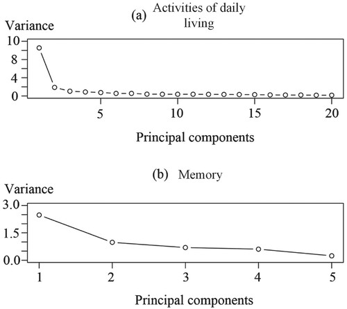
After calculating the eigenvalues and the principal components, the first few components are examined to determine if they account for a large proportion of the total variance. This study selects the components that account for more than 70% of cumulative variance. Figure 1 shows that the first principal components of both ADL and memory account for the overwhelming majority (over 70%) of the total variation in the original information. To balance between the number of components and the amount of original information, two principal components are used in subsequent analyses: the first principal components of ADL denoted as $\mathbf{\text{S}}$, and the first principal components of memory denoted as $\mathbf{\text{M}}$. The PCA transforming parameters of the two first principal components are shown in Tables 2 and 3.

3. Model formulation

3.1. Residual life prediction

Typically, deteriorating health means the reduction of residual life. Since health status is an ambiguous concept difficult to quantify, the residual life can be used as a health indicator. In this case, the health status information, including ADL and memory, is used to monitor our model. Generally, physical health is strongly associated with ADL, while mental health is positively related to memory; therefore, people in a feebler health status usually exhibit deteriorative performance in ADL and memory. Thus, there is a stochastic relationship between health status monitoring data and the unobserved actual health status.

In this study, a new filtering methodology with a recursive nature is adopted. The model use all past information about ADL and memory as covariates to predict residual life. From the PCA analyses, two principal components are shown to contain most of the initially observed information, and therefore, can be used to represent the original ADL and memory data. In practice, the first principal component means a weighted average of the original information where the weights are obtained by maximizing the variance. Let ${\mathbf{\text{S}}}_i$ denote the first principal components calculated based on the observed ADL at the time of the $i\text{th}$ survey, $t_i,$ let $x_i$ denote the residual life of the participant at $t_i$, provided that this individual has survived to $t_i$, and let ${\widetilde{\mathbf{\text{S}}}}_i$ denote the history values of $s_i$, where ${\widetilde{\mathbf{\text{S}}}}_i=\left\{s_1,s_2,\dots ,s_i\right\}$. ${\widetilde{\mathbf{\text{M}}}}_i$ is defined in the same pattern. Then the objective is to establish the Probability Distribution Function (PDF) of $x_i$ given ${\widetilde{\mathbf{\text{S}}}}_i$ and ${\widetilde{\mathbf{\text{M}}}}_i$, i.e. $p_i\left(x_i|{\widetilde{\mathbf{\text{S}}}}_i,{\widetilde{\mathbf{\text{M}}}}_i\right)$.

The relationship between residual lives at times $t_i$ and $t_{i-1}$ can be expressed as (3) $x_i=\left\{\begin{array}{ccc}{x}_{i-1}-\left(t_i-t_{i-1}\right)& \text{if }& x_{i-1}\ge t_i-t_{i-1}\text{,}\\ \text{not defined }& \text{if }& x_{i-1}<t_i-t_{i-1}\text{.}\end{array}\right.$(3) Equation (3) shows that $x_i$ must be conditional on $x_{i-1}\ge t_i-t_{i-1}$ so that $p_i\left(x_i|{\widetilde{\mathbf{\text{S}}}}_i,{\widetilde{\mathbf{\text{M}}}}_i,x_{i-1}\ge t_i-t_{i-1}\right)=p_i(x_i|{\widetilde{\mathbf{\text{S}}}}_i,{\widetilde{\mathbf{\text{M}}}}_i)$. Our model assumes that after obtaining the health status information (ADL and memory) at time $t_i$, the residual life distribution estimated is altered by the difference between the actual and expected health status decrements over $\left(t_{i-1},t_i\right)$. A similar concept has been used in accelerated life models where the survival function is accelerated by a deterministic constant (Crowder et al., 1991). Then $p_i\left(x_i|{\widetilde{\mathbf{\text{S}}}}_i,{\widetilde{\mathbf{\text{M}}}}_i,x_{i-1}\ge t_i-t_{i-1}\right)$ is given by (4) $\begin{array}{rl}& p_i\left(x_i|{\widetilde{\mathbf{\text{S}}}}_i,{\widetilde{\mathbf{\text{M}}}}_i,x_{i-1}\ge t_i-t_{i-1}\right)\\ & =p_i\left(x_i|{\widetilde{\mathbf{\text{S}}}}_i,{\widetilde{\mathbf{\text{M}}}}_i\right)\\ & =p_i\left(x_{i}f\left(\mathrm{\Delta }{w}_i-\mathrm{\Delta }{\overline{w}}_i\right)|{\widetilde{\mathbf{\text{S}}}}_{i-1},{\widetilde{\mathbf{\text{M}}}}_{i-1}\right)\frac{1}{f\left(\mathrm{\Delta }{w}_i-\mathrm{\Delta }{\overline{w}}_i\right)}\end{array}$(4) where $\mathrm{\Delta }{w}_i$ denotes the actual health status decrement and $\mathrm{\Delta }{\overline{w}}_i$ denotes the expected health status decrement over $\left(t_{i-1},t_i\right)$. Both $\mathrm{\Delta }{w}_i$ and $\mathrm{\Delta }{\overline{w}}_i$ may not be observed directly, but they can be indicated by $s_i$ and $m_i$ as $\mathrm{\Delta }{w}_i-\mathrm{\Delta }{\overline{w}}_i={\text{g}}_{\text{s}}\left(s_i-s_{i-1}-{\overline{s}}_i+{\overline{s}}_{i-1}\right)+{\text{g}}_{\text{m}}(m_i-m_{i-1}-{\overline{m}}_i+{\overline{m}}_{i-1})={\text{g}}_{\text{s}}\left(\mathrm{\Delta }{s}_i-\mathrm{\Delta }{\overline{s}}_i\right)+{\text{g}}_{\text{m}}\left(\mathrm{\Delta }{m}_i-\mathrm{\Delta }{\overline{m}}_i\right)$. Here, ${\overline{s}}_i$ and ${\overline{m}}_i$ denote expected $s_i$ and $m_i$, while $f$, ${\text{g}}_{\text{s}},$ and ${\text{g}}_{\text{m}}$ are functions $f\left(\mathrm{\Delta }{w}_i-\mathrm{\Delta }{\overline{w}}_i\right)=e^{-\left(\mathrm{\Delta }{w}_i-\mathrm{\Delta }{\overline{w}}_i\right)}$, ${\text{g}}_{\text{s}}\left(\mathrm{\Delta }{s}_i-\mathrm{\Delta }{\overline{s}}_i\right)=a\left(\mathrm{\Delta }{s}_i-\mathrm{\Delta }{\overline{s}}_i\right),$ respectively and ${\text{g}}_{\text{m}}(\mathrm{\Delta }{m}_i-\mathrm{\Delta }{\overline{m}}_i)=b(\mathrm{\Delta }{m}_i-\mathrm{\Delta }{\overline{m}}_i)$, where $a$ and $b$ are parameters to be specified.

The form of function $f\left(\mathrm{\Delta }{w}_i-\mathrm{\Delta }{\overline{w}}_i\right)$ is chosen based on the proportional hazard model. This model is a semi-parametric model with good performance in analysing and explaining the hazard for different values of the concerned variables. The form of function $f\left(\mathrm{\Delta }{w}_i-\mathrm{\Delta }{\overline{w}}_i\right)$ can be easily extended to other cases.

To calculate ${\text{g}}_{\text{s}}\left(\mathrm{\Delta }{s}_i-\mathrm{\Delta }{\overline{s}}_i\right)$ and ${\text{g}}_{\text{m}}\left(\mathrm{\Delta }{m}_i-\mathrm{\Delta }{\overline{m}}_i\right)$, we need first quantify the relationships between expected health status information (${\overline{\mathrm{s}}}_i$ and ${\overline{m}}_i$) and survival time ($t_i$) which also is the age when the participant was surveyed. We employed linear regression to quantify this relationship since the parameter estimation and prediction of linear regression are efficient, and the parameter in linear regression is easy to interpret. Thus, the two relationships can be expressed as ${\overline{\mathrm{s}}}_i=c_s{t}_i+d_s$ and ${\overline{m}}_i=c_m{t}_i+d_m$, where $c_s$, $d_s$, $c_m$ and $d_m$ are parameters. The form of the two relationships can be extended to other cases.

Then Equation (4) can be expressed as (5) $\begin{array}{rl}{p}_i\left(x_i|{\widetilde{\mathbf{\text{S}}}}_i,{\widetilde{\mathbf{\text{M}}}}_i\right)& =p_i\left(x_i{e}^{-a\left(\mathrm{\Delta }{s}_i-\mathrm{\Delta }{\overline{s}}_i\right)-b\left(\mathrm{\Delta }{m}_i-\mathrm{\Delta }{\overline{m}}_i\right)}|{\widetilde{\mathbf{\text{S}}}}_{i-1},{\widetilde{\mathbf{\text{M}}}}_{i-1}\right)\\ & \times e^{a\left(\mathrm{\Delta }{s}_i-\mathrm{\Delta }{\overline{s}}_i\right)+b\left(\mathrm{\Delta }{m}_i-\mathrm{\Delta }{\overline{m}}_i\right)}\end{array}$(5) which is a proportional function. If the health status is stable without deterioration, so that $\mathrm{\Delta }{s}_i-\mathrm{\Delta }{\overline{s}}_i=0$ and $\mathrm{\Delta }{m}_i-\mathrm{\Delta }{\overline{m}}_i=0$, then the residual life prediction should also be stable and $p_i\left(x_i|{\widetilde{\mathbf{\text{S}}}}_i,{\widetilde{\mathbf{\text{M}}}}_i\right)=p_i\left(x_i|{\widetilde{\mathbf{\text{S}}}}_{i-1},{\widetilde{\mathbf{\text{M}}}}_{i-1}\right)$. Otherwise, residual life prediction will vary proportionally with $\mathrm{\Delta }{s}_i-\mathrm{\Delta }{\overline{s}}_i$ and $\mathrm{\Delta }{m}_i-\mathrm{\Delta }{\overline{m}}_i$. By specifying an initial PDF of $x_0$, $p_0\left(x_0\right)$, and using the fact that (6) $p_i\left(x_i|{\widetilde{\mathbf{\text{S}}}}_{i-1},{\widetilde{\mathbf{\text{M}}}}_{i-1}\right)=\frac{p_i\left(x_i+t_i-t_{i-1}|{\widetilde{\mathbf{\text{S}}}}_{i-1},{\widetilde{\mathbf{\text{M}}}}_{i-1}\right)}{{\int }_{t_i-t_{i-1}}^{\mathrm{\infty }}{p}_i\left(u|{\widetilde{\mathbf{\text{S}}}}_{i-1},{\widetilde{\mathbf{\text{M}}}}_{i-1}\right)du},$(6) and Equation (5), after some recursive manipulations, it can be shown that the PDF of $x_i$ conditional on ${\widetilde{\mathbf{\text{S}}}}_{i-1}$ and ${\widetilde{\mathbf{\text{M}}}}_{i-1}$, and $x_i\ge t_i-t_{i-1}$ can be expressed as (7) $p_i\left(x_i|{\tilde{\mathbf{S}}}_i,{\tilde{\mathbf{M}}}_i\right)=\frac{\begin{array}{c}{p}_i\left(x_i\right.\\ e^{a\left(s_i-{\overline{\mathrm{s}}}_i\right)+b\left(m_i-{\overline{m}}_i\right)}\\ +\sum _{k=2}^i\left(t_k-t_{k-1}\right)\\ \left.e^{a\left(s_i-{\overline{s}}_{i-1}\right)+b\left(m_i-{\overline{m}}_{i-1}\right)}+t_1\right)\\ e^{a\left(\mathrm{\Delta }{s}_i-\mathrm{\Delta }{\overline{s}}_i\right)+b\left(\mathrm{\Delta }{m}_i-\mathrm{\Delta }{\overline{m}}_i\right)}\end{array}}{\begin{array}{c}{\int }_{t_i-t_{i-1}}^{\mathrm{\infty }}{p}_0\\ \left(u{e}^{a\left(s_i-{\overline{s}}_{i-1}\right)+b\left(m_i-{\overline{m}}_{i-1}\right)}\right.\\ +\sum _{k=2}^{i-1}\left(t_k-t_{k-1}\right)\\ \left.e^{a\left(s_i-{\overline{s}}_{i-1}\right)+b\left(m_i-{\overline{m}}_{i-1}\right)}+t_1\right)du\end{array}}.$(7) Equation (7) shows an advantage of this model: $x_k$ is conditional on all past $s_k$ and $m_k$, $k=1,2,...,i$, rather than just the current $s_i$ and $m_i$. If all $\mathrm{\Delta }{s}_i-\mathrm{\Delta }{\overline{s}}_i=0$ and $\mathrm{\Delta }{m}_i-\mathrm{\Delta }{\overline{m}}_i=0$, this equation then returns to the conventional conditional survival PDF. If all observed data conform to the expected mean, then $p_i\left(x_i|{\widetilde{\mathbf{\text{S}}}}_{\mathit{i}},{\widetilde{\mathbf{\text{M}}}}_{\mathit{i}}\right)=p_0\left(x_i+t_i\right)/{\int }_{t_i}^{\mathrm{\infty }}{p}_0\left(u\right)du$ as there is no evidence of deviation from the original prediction. Only in some cases when $\mathrm{\Delta }{\text{s}}_i-\mathrm{\Delta }{\overline{s}}_i\ne 0$ or $\mathrm{\Delta }{m}_i-\mathrm{\Delta }{\overline{m}}_i\ne 0$, $p_i\left(x_i|{\widetilde{\mathbf{\text{S}}}}_{\mathit{i}},{\widetilde{\mathbf{\text{M}}}}_{\mathit{i}}\right)$ $\text{is}$ revised accordingly. However, it should be noted that this is not the case in using the proportional hazard model, where the hazard can only return to the baseline hazard if all $s$ and $m=0$. There is no difficulty in extending the model to use more principal components. However, for the balance between the accuracy and the number of parameters estimated, this study focuses on the case where only the two most important principal components are used.

For the initial residual life distribution $p_0\left(x_0\right)$, an appropriate choice is the Weibull distribution, $p_0\left(x_0\right)={\alpha }^{\text{β}}\text{β}{x}_0^{\text{β}-1}{e}^{-{\left(\alpha x_0\right)}^{\text{β}}}$, where $\alpha$ is the scale parameter and $\text{β}$ is the shape parameter. The Weibull distribution is a widely used survival analysis distribution. The closed-form of the survival function and the wide variety of shapes exhibited by density functions make the Weibull distribution a particularly convenient generalization of the exponential distribution. It can be used to flexibly describe time distribution, especially when the hazard rate may increase, decrease, or remain invariant.

3.2. Parameter estimation

There are three sets of parameters estimated in our model, as shown in Table 4. The first set includes the Weibull distribution $p_0\left(x_0\right)$ that includes the scale parameter $\alpha$ and the shape parameter $\text{β}$. If there are enough residual life data, the two parameters can be estimated using the maximum likelihood method. From the available information sources, among the $n$ participants’ life data, $h$ of them are complete life data, and the $h_c$ of them are censored data, then the likelihood function is $L=\left\{{\prod }_{j=1}^{h}f\left(t_{jf}\right)\right\}\left\{{\prod }_{l=1}^{h_c}s\left(t_l\right)\right\}$, where $f$ is the PDF of lifetime, $s$ is the survival function, $t_{jf}$ is the final lifespan of the $i$th participants, and $t_l$ is the last survey time of the $l$th censored participant. The estimated values of the scale parameter $\alpha$ and the shape parameter $\text{β}$ can be obtained by maximizing the likelihood function.

Table 4. Parameter estimated.

Parameter set	Parameters
1	$\alpha$, $\text{β}$
2	$c_s$, $d_s$, $c_m$, $d_m$
3	$a$, $b$

The second set is within the linear regression for the relationships between health status information and survival time, including $c_s$, $d_s$, $c_m$, and $d_m$. The estimation for this parameter set is conducted based on the available data. In practice, the parameters in the second set can also be adjusted by health workers’ experience.

The third set includes the parameters $a$ and $b,$ which govern the relation between $x_i$ and $\mathrm{\Delta }{w}_i,$ and they are called governor parameters. The two parameters are the core parameters in the proposed model, and they are estimated by the following method.

For any participant, the following events have been observed at each survey: $x_{i-1}\ge t_i-t_{i-1}$ if the participant is alive; or $x_n\ge t_f-t_n$, where $t_f$ is the lifespan and $t_n$ is the time of the last survey before $t_f$. The likelihood function of all observed events for a participant is (8) $\begin{array}{rl}L& =p_0\left(x_0>t_1\right)\times p_1\left(x_1>t_2-t_1|{\text{s}}_1\right)\\ & \times p_{n-1}\left(x_{n-1}>t_{n-1}-t_{n-2}|{\text{s}}_{n-1}\right)\\ & \times p_n\left(x_n=t_f-t_n|s_n\right).\end{array}$(8) Note that these events are all conditioned on the participant having survived up to the time of the events, so the events are statistically independent. Using Equation (7) after some manipulations, the likelihood function for a single participant over his or her lifetime can be expressed as (9) $\begin{array}{rl}L& =p_0\left(\phantom{\sum _{n=1}^N}\left(t_f-t_n\right)e^{a\left(s_n-{\overline{s}}_n\right)+b\left(m_n-{\overline{m}}_n\right)}\right.\\ & +\left.\sum _{k=2}^n\left(t_k-t_{k-1}\right)e^{a\left(s_i-{\overline{s}}_{i-1}\right)+b\left(m_i-{\overline{m}}_{i-1}\right)}+t_1\right)\\ & \times {e^{\left(a\right(}}^{\mathrm{\Delta }{s}_i-\mathrm{\Delta }{\overline{s}}_i)+b(\mathrm{\Delta }{m}_i-\mathrm{\Delta }{\overline{m}}_i\left)\right)}.\end{array}$(9) The likelihood function for h participants is given by (10) $\begin{array}{rl}L& ={\prod }_{j=1}^h\left\{\phantom{\sum _{n=1}^N}{p}_0\left(\phantom{\sum _{n=1}^N}\left(t_{jf}-t_{j{n}_j}\right)e^{a\left(s_{j{n}_j}-{\overline{s}}_{j{n}_j}\right)+b\left(m_{j{n}_j}-{\overline{m}}_{j{n}_j}\right)}\right.\right.\\ & \left.+\sum _{k=2}^{n_j}\left(t_{jk}-t_{j,k-1}\right)e^{a\left(s_{j,k-1}-{\overline{s}}_{j,k-1}\right)+b\left(m_{j,k-1}-{\overline{m}}_{j,k-1}\right)}+t_{j1}\right)\\ & \times \left.\phantom{\sum _{n=1}^N}{e}^{a\left(\mathrm{\Delta }{s}_{j{n}_j}-\mathrm{\Delta }{\overline{s}}_{j{n}_j}\right)+b\left(\mathrm{\Delta }{m}_{j{n}_j}-\mathrm{\Delta }{\overline{m}}_{j{n}_j}\right)}\right\}\end{array}$(10) where $t_{jf}$ is the lifespan of the $j$th participant, $t_{jk}$ is the time of the $k$th survey of the $j$th participant, $s_{jk}$ and $m_{jk}$ are the first principal components of the $j$th participant at $t_{jk}$, and $n_j$ is the number of surveys before the death of the $j$th participant.

Equation (10) represents the probability that all the events reflected by the data happened. Herein, once we have the first two sets of parameters, the values of $a$ and $b$ can be estimated by maximizing the logarithm of Equation (10).

4. Model fitting

4.1. Fitting the model to the data

In this section, the model introduced above is fitted to the health status data from the CHNS. To keep as much as the original information as possible, both the complete and censored samples are used; 9566 randomly selected samples were to fit the model and the remaining 1420 samples were used to test the fitted model. Since the ADL and memory test information are only collected from people aged 55 and older, all the fitting analyses are limited to this population. Participants observed after the age of 55, $p\left(t\ge 55\right)=1$ and $p\left(x|t\ge 55\right)=p\left(x\right)$. For simplicity, the survival time $t$ is calculated from age 55, that is $t_i=\text{the age of }i\text{th survey}-55$.

For the initial residual life distribution $p_0\left(x_0\right)$, where $p_0\left(x_0\right)={\alpha }^{\text{β}}\text{β}{x}_0^{\text{β}-1}{e}^{-{\left(\alpha x_0\right)}^{\text{β}}}$, the scale parameter $\alpha$ and the shape parameter $\text{β}$ of the Weibull distribution are estimated using the maximum likelihood method based on data from 9566 samples. Incorporating the Weibull distribution into the likelihood function can beexpressed as (11) $\begin{array}{rl}L& =\left\{\prod _{j=1}^{h}f\left(t_{jf}\right)\right\}\left\{\prod _{l=1}^{h_c}s\left(t_l\right)\right\}\\ & =\left\{\prod _{j=1}^h{\alpha }^{\text{β}}\text{β}{t}_{jf}^{\text{β}-1}{e}^{-{\left(\alpha t_{jf}\right)}^{\text{β}}}\right\}\left\{\prod _{l=1}^{h_c}{e}^{-{\left(\alpha t_l\right)}^{\text{β}}}\right\},\end{array}$(11) where $t_{jf}$ is the life span of the $j$th complete participant and $t_l$ is the last survey time of the $l$th censored participant. Taking the logarithm on both sides of Equation (11), it can be transformed to (12) $\begin{array}{rl}\text{Ln}L& =h\text{β}\log \alpha +h\log \text{β}\\ & +\sum _{(j=1)}^h\left\{(\text{β}-1)\text{log}{t}_{jf}-{\left(\alpha t_{jf}\right)}^{\text{β}}+\right\}\\ & +\sum _{(j=1)}^h\left\{-{\left(\alpha t_l\right)}^{\text{β}}\right\}.\end{array}$(12) By maximizing Equation (12), the estimates of $\alpha$ and $\text{β}$ are $\hat{\alpha }=0.033494$ and $\widehat{\text{β}}=2.896380$, respectively; by inverting the information matrix, the variances and covariance of estimated parameters $\alpha$ and $\text{β}$ can be approximated, then $\text{Var}\left(\alpha \right)=5.98\times {10}^{-8}$, $\text{Var}\left(\text{β}\right)=1.65\times {10}^{-8}$ and $\text{Cov}\left(\alpha ,\text{β}\right)=6.25\times {10}^{-5}$. The variances and the covariance of the estimated $\alpha$ and $\text{β}$ are minimal compared with their estimated values, which means that they are stable and probably uncorrelated.

The health status information and survival time relationships are expressed as ${\overline{\mathrm{s}}}_i=c_s{t}_i+d_s$ and ${\overline{m}}_i=c_m{t}_i+d_m$. The results of the regression show that $c_s=0.13$, $d_s=4.48$, $c_m=0.15$ and $d_m=-3.28$ and all the regression parameters are significant (P-Value $<2\times {10}^{-5}$). In other words, with age (survival time) increase, the ADL and memory will deteriorate.

Next, parameters $a$ and $b$ can be estimated using the maximum likelihood method as (13) $\begin{array}{rl}L& =\prod _{j=1}^h\left\{\phantom{\prod _{k=2}^{n_l}}{p}_0\left(x_0>t_{j1}\right)\right.\\ & \times \left(\prod _{k=2}^{n_j}{p}_{k-1}\left(x_{k-1}>t_{jk}-t_{jk-1}|{\tilde{\mathrm{S}}}_{j,k-1},{\tilde{\mathrm{M}}}_{j,k-1}\right)\right)\\ & \times \left.p_{n_j}\left(x_{n_j}=t_{jf}-t_{n_j}|{\tilde{\mathrm{S}}}_{j{n}_j},{\tilde{\mathrm{M}}}_{j{n}_j}\right)\phantom{\prod _{k=2}^{n_l}}\right\}\\ & \times \prod _{l=1}^{h_c}\left\{p_0\left(x_0>t_{l1}\right)\times \left(\prod _{k=2}^{n_l}{p}_{k-1}(x_{k-1}>t_{lk}-t_{lk-1}\right.\right.\\ & \left.\times \left.|{\tilde{\mathrm{S}}}_{l,k-1},{\tilde{\mathrm{M}}}_{l,k-1})\phantom{\prod _{k=2}^{n_l}}\right)\right\},\end{array}$(13) where ${\tilde{\mathrm{S}}}_{\cdot ,k}=\left[s_{\cdot ,1},\dots ,s_{\cdot ,k}\right]$ and ${\tilde{\mathrm{M}}}_{\cdot ,k}=\left[m_{\cdot ,1},\dots ,m_{\cdot ,k}\right]$. Using Equation (7), $p_0\left(x_0\right)$, and taking ln on both sides of Equation (13), it can be expressed as (14) $\begin{array}{rl}\text{Ln}L& =h\text{β}\ln \alpha +h\ln \text{β}\\ & +\sum _{j=1}^h\left\{\phantom{\prod _{k=2}^{n_l}}a\left(\mathrm{\Delta }{s}_{n_j}-\mathrm{\Delta }{\overline{s}}_{n_j}\right)+b\left(\mathrm{\Delta }{m}_{n_j}-\mathrm{\Delta }{\overline{m}}_{n_j}\right)\right.\\ & +\left(\text{β}-1\right)\ln \left(\sum _{k=2}^{n_j+1}{\mathrm{\Lambda }}_{j,k-1}\left(t_{jk}-t_{j,k-1}\right)+t_1\right)\\ & \left.-{\left(\alpha \left(\sum _{k=2}^{n_j}{\mathrm{\Lambda }}_{j,k-1}\left(t_{jk}-t_{j,k-1}\right)+t_{j1}\right)\right)}^{\text{β}}\right\}\\ & -\sum _{l=2}^{n_l}{\left\{\alpha \left(\sum _{k=2}^{n_l}{\mathrm{\Lambda }}_{l,k-1}\left(t_{lk}-t_{l,k-1}\right)+t_{l1}\right)\right\}}^{\text{β}},\end{array}$(14) where ${\mathrm{\Lambda }}_{\cdot ,k}=e^{a\left(z_{\cdot k}-{\overline{z}}_{\cdot k}\right)}$ and $t_{jf}=t_{n_j+1}$. By maximizing Equation (14), the estimated values of $\hat{a}=1.58\times {10}^{-2}$ and $\hat{b}=1.49\times {10}^{-2}$, given that $\alpha$ and $\text{β}$ are substituted by their estimated values $\hat{\alpha }$ and $\widehat{\text{β}}$. The variance of the estimated parameter $a$ is calculated by $\text{Var}\left(a\right)\approx -\text{E}({\mathrm{\partial }}^2\ln L/\mathrm{\partial }{a}^2{)}^{-1}$. $\text{Var}\left(b\right)$ and $\text{Cov}\left(a,b\right)$ can also be calculated in the same way. Then we have $\text{Var}\left(a\right)=6.14\times {10}^{-5}$, $\text{Var}\left(b\right)=7.25\times {10}^{-5}$ and $\text{Cov}\left(a,b\right)=9.71\times {10}^{-5}$. For $a\text{and}b$, the calculated variances and co-variances are extremely small compared with the estimated values, so that they are stable and uncorrelated.

The residual life of a participant at time $t_i$ is predicted based upon estimated model parameters and the information of first two principal components. The ${\mathit{p}}_{\mathit{i}}\left({\mathit{x}}_{\mathit{i}}|{\widetilde{\mathbf{\text{S}}}}_{\mathit{i}},{\widetilde{\mathbf{\text{M}}}}_{\mathit{i}}\right)$ is expressed by the following function: (15) $\begin{array}{rl}& p_i\left(x_i|{\tilde{\mathbf{S}}}_i,{\tilde{\mathbf{M}}}_i\right)\\ & =\frac{\begin{array}{c}{\alpha }^{\text{β}}\text{β}{\left(x_i{\mathrm{\Lambda }}_i+\sum _{k=2}^i{\mathrm{\Lambda }}_{k-1}\left(t_k-t_{k-1}\right)+t_1\right)}^{\text{β}-1}\\ e^{-{\left(\alpha \left(x_i{\mathrm{\Lambda }}_i+\sum _{k=2}^i{\mathrm{\Lambda }}_{k-1}\left(t_k-t_{k-1}\right)+t_1\right)\right)}^{\text{β}}}\\ e^{a\left(\mathrm{\Delta }{s}_i-\mathrm{\Delta }{\overline{s}}_i\right)+b\left(\mathrm{\Delta }{m}_i-\mathrm{\Delta }{\overline{m}}_i\right)}\end{array}}{\begin{array}{c}{e}^{-{\left(\alpha \left(\sum _{k=2}^i{\mathrm{\Lambda }}_{k-1}\left(t_k-t_{k-1}\right)+t_1\right)\right)}^{\text{β}}}\\ e^{-a\left(s_i-{\overline{s}}_i\right)+b\left(m_i-{\overline{m}}_i\right)}\end{array}}\end{array}$(15) This equation shows a life mechanism that predicts how residual life is influenced by the deviation between the expected and real components’ information, while increasing health status deterioration indicates a relatively shorter residual life.

4.2. Goodness-of-fit

To assess the model fit, 1420 samples were chosen as test set and the chi-square goodness-of-fit test $\left({\chi }^2\right)$ was used to carry out the test (Fisher, 1922; Pearson, 1992). This study of the chi-squared test is not applied since there is only one observation for each distribution $p_i\left(x_i|{\widetilde{\mathbf{\text{S}}}}_{\mathit{i}},{\widetilde{\mathbf{\text{M}}}}_{\mathit{i}}\right)$. It is feasible to carry out the chi-squared test in this situation by partitioning each distribution $p_i\left(x_i|{\widetilde{\mathbf{\text{S}}}}_{\mathit{i}},{\widetilde{\mathbf{\text{M}}}}_{\mathit{i}}\right)$ into some intervals with equal probability; then $x_i$ will have an equal probability to be in any one of the intervals. This effectively transforms $x_i$ into a uniform distribution. Specifically, $x_i$ is partitioned into $N$ cells here so that each cell had an equal probability, $p=1/N$. Under the hypothesized distribution, each observation cell is examined. After this transformation, all $x_i$ follow an identical uniform distribution, the number of observations $G$ per cell counted and compared with the expected values followed by goodness-of-fit test.

However, for the censored participants, their real residual life cannot be known at each survey. For these samples, $p_i\left(x_i>t_l|{\widetilde{\mathbf{\text{S}}}}_{\mathit{i}},{\widetilde{\mathbf{\text{M}}}}_{\mathit{i}}\right)$ is calculated and the $x_i$ is assumed to have an equal probability of being in any one of the $K$ cells covered by $p_i\left(x_i>t_l|{\widetilde{\mathbf{\text{S}}}}_{\mathit{i}},{\widetilde{\mathbf{\text{M}}}}_{\mathit{i}}\right)$. In this case, all the numbers of observations in these $K$ cells increase by $1/K$.

The null hypothesis $H_0$ is that the elderly’s residual life $x_i$ follows the stated probability distribution $p_i\left(x_i|{\widetilde{\mathbf{\text{S}}}}_{\mathit{i}},{\widetilde{\mathbf{\text{M}}}}_{\mathit{i}}\right)$. Since all parameters in $p_i\left(x_i|{\widetilde{\mathbf{\text{S}}}}_{\mathit{i}},{\widetilde{\mathbf{\text{M}}}}_{\mathit{i}}\right)$ are already estimated by the other 9566 randomly selected samples, the hypothesis here is simple. To do the test, we need to decide the number of partitions, namely, $N$. It is recommended that for a sample of size $n$ (large) and significance level $\alpha =0.05$, one should use approximately $N=2n^{2/5}$ (D’Agostino & Stephens, 1986). Then the expected number of observations in each cell is $np=n/N,$ and finally, the sum of standard deviation can be expressed by (16) $\text{Sum}=\sum _{i=1}^N\frac{{\left(G_i-np\right)}^2}{np}=\sum _{i=1}^N\frac{{\left(G_i-n/N\right)}^2}{n/N}$(16)

In this study, $N\approx 2n^{2/5}=36.47$, thus choosing $N=36$ is reasonable. Then the degree of freedom is $36-2=34$, the equal probability of each cell $p$ is $1/36,$ and the expected number of observations in each cell is $np=1420/36=39.44$. Substituting these values into Equation (16), the sum of standard deviation is 32.43. On the other hand, if we choose a significance level of 0.05, referring to the ${\chi }^2$ table, the critical value is ${\chi }_{0.95}^2\left(34\right)=48.60$. As 32.43 is smaller than 48.60, the hypothesis is true, so that there is no evidence to reject the established model.

5. Case study

In this section, a participant was chosen as an example to exhibit the fitted model. The participant was first surveyed when he was 61 years old and the subsequent surveys were carried out at the ages of 65, 68, 72, and 74. Finally, he passed away just ten months after the last survey. The residual life distribution of the participant was predicted after each survey based on his ADL and memory information using the model fitted in Section 6.

To illustrate the effectiveness of the proposed model, two perspectives of comparisons are provided based on this example: (1) the fitted model itself, including the comparisons for the result from the initial distribution (Weibull distribution) before using the proposed model and the result from using exponential distribution instead of Weibull distribution as the initial distribution in the fitted model; (2) the proposed model vs. other prediction methods, including the comparisons for the result from multiple regression and the result from the life table.

5.1. The proposed model

To provide the effectiveness in terms of the proposed model itself, we calculate the results from two methods: (1) the initial distribution using the Weibull distribution without the stochastic filtering; (2) exponential distribution as the initial distribution that is using exponential distribution to replace the Weibull distribution as the initial distribution.

5.1.1. Comparison with initial distribution (Weibull distribution)

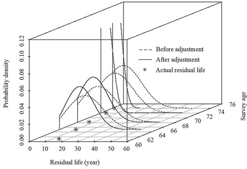
This comparison shows the difference between the results from the fitted model and the initial distribution (before adjustment, Weibull distribution), as shown in Figure 2. The residual life prediction using the fitted model in this study is more accurate than the initial distribution in general. The Mean Square Error (MSE) is also calculated. The MSE using our model is 6.2, and without it is 66.3. This proves that the fitted model provides a more reasonable prediction distribution. In addition, with increasing survey times and information amount, the fitted model is more precise and stable. The fitted model work only after the second survey because both $\mathrm{\Delta }{w}_i$ and $\mathrm{\Delta }{\overline{w}}_i$ used in this model need at least two observations to calculate.

Figure 2. Comparison of the predicted residual life distribution based on the fitted model and the initial distribution. (Note: the distribution curves of the fourth and fifth predictions are too centralized to be shown in the plot, so the last two curves are interrupted; the following figures also have the similar situations).

5.1.2. Comparison with exponential distribution as the initial distribution

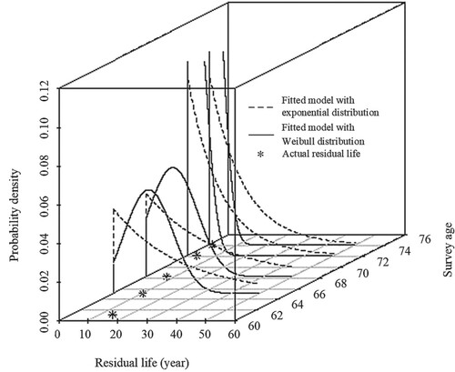
The exponential distribution is widely used to depict the residual life, especially those whose residual life is irrelevant to their history. Thus, this comparison shows the difference between the results from the fitted model with the Weibull or the exponential distribution as the initial distribution, as shown in Figure 3.

Figure 3. Comparison of the predicted residual life distribution based on the fitted model with Weibull distribution and the fitted model with exponential distribution.

In this study, the exponential distribution is fitted with the same data from the Weibull distribution, which is $\left(1/\theta \right){\text{e}}^{\left(-x/\theta \right)}$, where $\theta =0.034494$. The residual life prediction using the fitted model with Weibull distribution is more accurate than with an exponential distribution. This proves that using the Weibull distribution in the fitted model provides a more reasonable prediction than the exponential distribution.

5.2. The proposed model vs. other prediction methods

To further illustrate the proposed model’s effectiveness, we further provide the results from other methods of residual life prediction as comparative studies. Among the life prediction methods for human beings, regression analysis and life table are the two most commonly used methods. Regression analysis is a classical and straightforward statistical method to conduct prediction, especially for predicting with a large amount of data. The life table is a statistical table reflecting the death of a group of people (usually 10,000 people), compiled according to the age-specific mortality. The comparisons of the proposed model using multiple regression and life table are presented below.

5.2.1. Comparison with multiple linear regression

The formula of the multiple linear regression is $x_i=l_s{s}_i+l_m{m}_i+l_a+ϵ$, where $l_a$ is the constant, $ϵ$ is the random error following $N\left(0,{\sigma }^2\right)$, $l_s$ and $l_m$ are the coefficients of the first principle components of ADL and memory, respectively. Using the same data as in the fitting for the proposed model, the values of $l_a$, $l_s$, $l_m,$ and $\sigma$ can be estimated to 6.55318, 0.26129, 0.07349, and 0.25761, respectively. Then we used this multiple linear regression model to predict the residual life, $\widehat{x_i}$. According to the linear regression, the prediction distribution is a normal distribution $N\left(\widehat{x_i},{\sigma }^2\right)$. Finally, we compared the difference between the results from the fitted model and the multiple regression, as shown in Figure 4.

Figure 4. Comparison of the predicted residual life distributions from the proposed model and multiple linear regression.

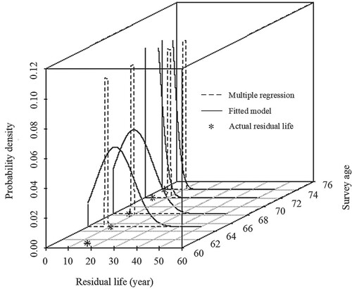
The residual life prediction using the proposed model is more accurate than using multiple linear regression, especially at the last two survey times when more historical health information was collected and integrated into the model.

5.2.2. Comparison with life table

Since the survey data ended in 2011, we use the 2010 life table of the Chinese population, as shown in Table 5. To provide a comparison, a normal distribution, based on a Life Table, is presented. The expectation is the residual life from the Life Table, while the standard deviation is set as 1 since the expected residual life is updated with age annually. Thus, we compare the difference between the fitted model and life table results, respectively, as shown in Figure 5.

Figure 5. Comparison of the predicted residual life distribution based on the fitted model with Weibull distribution and the fitted model with exponential distribution.

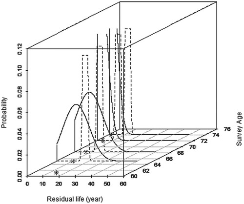
Table 5. Life table of Chinese population in 2010.

Age	Expected residual life
61	20.76
65	17.62
68	15.39
72	12.72
74	11.50

Our results show that the residual life prediction using the proposed model is more accurate than using a life table. Generally, residual life prediction from the life table is longer, and the proposed model can update the prediction according to the historical health information compared with the life table.

6. Discussion

The proposed model in this study is based on the stochastic filtering theory, which solves drawbacks of quantitative analysis of the previous statistical models. The proposed model can use time-series data through a recursive method to constantly update the prediction and improve its reliability. In terms of the data, ADL and memory were used to extract an indicator that comprehensively reflects people’s health status. This method is different from the previous health assessment using biochemical indicators. The information we used is a more comprehensive reflection of health level, emphasizing the ability to live. This method is more conducive to promotion and application, especially in economically underdeveloped areas with poor medical conditions.

According to the research results, ADL and memory are adequate information for calculating the remaining human life. With the deterioration of health, residual life will decrease, and at the same time, ADL and memory will worsen. If ADL and memory reflect the acceleration of this trend, residual life will also be accelerated until the end of life. This implies that society should pay more attention to people’s ADL and memory to guard against health deterioration. In addition, for health management agencies and insurance companies, ADL and memory should also become important references for guiding work.

7. Conclusions

This study presents an improved method to estimate the residual life of the elderly by using a recursive model. Compared to the previous study model, the proposed model is developed to integrate the health information extracted from ADL and memory, which is the progressive feature of this study. This paper provides a physiologic relationship between the health status and ADL and memory. When memory is introduced as a mental factor, the usage and feasibility of the stochastic filtering are further verified. As ageing is an increasingly serious issue in many countries, the government and the public should pay attention to the ADL and memory of the elderly.

There are two possible limitations of the proposed method. On the one hand, the method is a little complex in terms of its mathematical calculation. However, this limitation can be addressed by developing this method into algorithms and models embedded in the software. On the other hand, the accuracy and precision of the prediction by this method increases with the quantity of historical information, so that this method requires an effective health information recording system or organization.

This article can be extended in a few directions. One direction is to extend the method for the application to the young population. Another direction is to apply this method to other survey data where the health information may be different. Also, it is also meaningful to study the optimization of health behaviour based on the prediction of the proposed method.

Disclosure statement

No potential conflict of interest was reported by the author(s).

Additional information

Funding

This research was funded by the National Natural Science Foundation of China [grant number 72001027] and Beijing Municipal Education Commission [grant number KM202111232007].

References

- Arora, A., Spatz, E., Herrin, J., Riley, C., Roy, B., Kell, K., Coberley, C., Rula, E., & Krumholz, H. M. (2016). Population well-being measures help explain geographic disparities in life expectancy at the county level. Health Affairs, 35(11), 2075–2082. https://doi.org/https://doi.org/10.1377/hlthaff.2016.0715
- Atance, D., Debón, A., & Navarro, E. (2020). A Comparison of forecasting mortality models using resampling methods. Mathematics, 8(9), 1550. https://doi.org/https://doi.org/10.3390/math8091550
- Beard, J., & Bloom, D. (2015). Towards a comprehensive public health response to population ageing. The Lancet, 385(9968), 658–661. https://doi.org/https://doi.org/10.1016/S0140-6736(14)61461-6
- Boudoulas, K. D., Triposkiadis, F., Stefanadis, C., & Boudoulas, H. (2017). The endlessness evolution of medicine, continuous increase in life expectancy and constant role of the physician. Hellenic Journal of Cardiology, 58(5), 322–330. https://doi.org/https://doi.org/10.1016/j.hjc.2017.05.001
- Brewer, W. J., Francey, S. M., Wood, S. J., Pantelis, H. J., Phillips, L. J., Yung, A. R., Anderson, V. A., & McGorry, P. D. (2005). Memory impairments identified in people at ultra-high risk for psychosis who later develop first-episode psychosis. American Journal of Psychiatry, 162(1), 71–78. https://doi.org/https://doi.org/10.1176/appi.ajp.162.1.71
- Cho, G., Kim, D., Jung, S., Jung, I. H., & Kim, S. (2020). Estimating age-specific natural mortality for sandfish in the eastern coastal waters of Korea. Mathematics, 8(9), 1612. https://doi.org/https://doi.org/10.3390/math8091612
- Covinsky, K. E., Palmer, R. M., Fortinsky, R. H., Counsell, S. R., Stewart, A. L., Kresevic, D., & Burant, C. J. (2003). Loss of independence in activities of daily living in older adults hospitalized with medical illnesses: Increased vulnerability with age. Journal of the American Geriatrics Society, 51(4), 451–458. https://doi.org/https://doi.org/10.1046/j.1532-5415.2003.51152.x
- Crowder, M. J., Kimber, A. C., Smith, R. L., & Sweeting, T. J. (1991). Statistical analysis of reliability data. Chapman and Hall.
- D’Agostino, R. B., & Stephens, M. A. (1986). Goodness-of-fit-techniques. Marcel Dekker.
- de Cabo, R., & Mattason, M. P. (2019). Effects of intermittent fasting on health, aging, and disease. New England Journal of Medicine, 381(26), 2541–2551. https://doi.org/https://doi.org/10.1056/NEJMra1905136.
- DESA. (2007). Development in an ageing world. World economic and social survey (pp. v–viii). United Nations. http://citeseerx.ist.psu.edu/viewdoc/download;jsessionid=2302B1B61C64FB890F208EB0DD218401?doi=10.1.1.177.2319&rep=rep1&type=pdf
- Díaz-Rojo, G., Debón, A., & Mosquera, J. (2020). Multivariate control chart and Lee–Carter models to study mortality changes. Mathematics, 8(11), 2093. https://doi.org/https://doi.org/10.3390/math8112093
- Dunlop, D., Hughes, S., & Manheim, L. (1997). Disability in activities of daily living: Patterns of change and a hierarchy of disability. American Journal of Public Health, 87(3), 378–383. https://doi.org/https://doi.org/10.2105/AJPH.87.3.378
- Evans, G. F., & Soliman, E. Z. (2019). Happier countries, longer lives: An ecological study on the relationship between subjective sense of well-being and life expectancy. Global Health Promotion, 26(2), 36–40. https://doi.org/https://doi.org/10.1177/1757975917714035
- Fisher, R. (1922). On the interpretation of χ2 from contingency tables, and the calculation of P. Journal of the Royal Statistical Society, 85(1), 87–94. https://doi.org/https://doi.org/10.2307/2340521
- Fitzmaurice, C., Abate, D., Abbasi, N., Abbastabar, H., Abd-Allah, F., Abdel-Rahman, O., Abdelalim, A., Abdoli, A., Abdollahpour, I., Abdulle, A. S. M., Abebe, N. D., Abraha, H. N., Abu-Raddad, L. J., Abualhasan, A., Adedeji, I. A., Advani, S. M., Afarideh, M., Afshari, M., Aghaali, M., & Agius, D. (2019). Global, regional, and national cancer incidence, mortality, years of life lost, years lived with disability, and disability-adjusted life-years for 29 cancer groups, 1990 to 2017 a systematic analysis for the Global Burden of Disease Study. JAMA Oncology, 5(12), 1749–1768. https://doi.org/https://doi.org/10.1001/jamaoncol.2019.2996
- Gregersen, F. (2014). The impact of ageing on health care expenditures: A study of steepening. The European Journal of Health Economics, 15(9), 979–989. https://doi.org/https://doi.org/10.1007/s10198-013-0541-9
- Hashir, M., & Sawhney, R. (2020). Towards unstructured mortality prediction with free-text clinical notes. Journal of Biomedical Informatics, 108, 103489. https://doi.org/https://doi.org/10.1016/j.jbi.2020.103489
- Jagger, C., Matthews, R., Matthews, F., Robinson, T., Robine, J. M., Brayne, C., & Medical Research Council Cognitive Function and Ageing Study Investigators. (2007). The burden of diseases on disability-free life expectancy in later life. The Journals of Gerontology Series A: Biological Sciences and Medical Sciences, 62(4), 408–414. https://doi.org/https://doi.org/10.1093/gerona/62.4.408
- Katz, S. (1983). Assessing self-maintenance: Activities of daily living, mobility, and instrumental activities of daily living. Journal of the American Geriatrics Society, 31(12), 721–727. https://doi.org/https://doi.org/10.1111/j.1532-5415.1983.tb03391.x
- Li, R., & Liu, Y. (2020). Sparse representation-based classification for the planetary gearbox with improved KPCA and dictionary learning. Systems Science & Control Engineering, 8(1), 369–379. https://doi.org/https://doi.org/10.1080/21642583.2020.1777218
- Li, X., Liu, H. F., Yang, J. G., Xie, G. T., Xu, M. L., & Yang, Y. J. (2017). Using machine learning models to predict in-hospital mortality for ST-elevation myocardial infarction patients. Studies in Health Technology and Informatics, 245, 476–480. https://doi.org/https://doi.org/10.3233/978-1-61499-830-3-476
- Liu, D., Wang, Z. D., Liu, L. R., & Alsaadi, F. E. (2021). Recursive filtering for stochastic parameter systems with measurement quantizations and packet disorders. Applied Mathematics and Computation, 398, 125960. https://doi.org/https://doi.org/10.1016/j.amc.2021.125960
- Lubitz, J., Cai, L., Kramarow, E., & Lentzner, H. (2003). Health, life expectancy, and health care spending among the elderly. New England Journal of Medicine, 349(11), 1048–1055. https://doi.org/https://doi.org/10.1056/NEJMsa020614
- McGuire, L., Ford, E., & Ajani, U. (2006). Cognitive functioning as a predictor of functional disability in later life. The American Journal of Geriatric Psychiatry, 14(1), 36–42. https://doi.org/https://doi.org/10.1097/01.JGP.0000192502.10692.d6
- Miao, C., & Lv, Z. (2020). Nonlinear chemical processes fault detection based on adaptive kernel principal component analysis. Systems Science & Control Engineering, 8(1), 350–358. https://doi.org/https://doi.org/10.1080/21642583.2020.1768173
- Oliver, D., Foot, C., & Humphries, R. (2014). Making our health and care systems fit for an ageing population. King’s Fund.
- Parker, M., Bucknall, M., Jagger, C., & Wilkie, R. (2020). Extending working lives: A systematic review of healthy working life expectancy at age 50. Social Indicators Research, 150(1), 337–350. https://doi.org/https://doi.org/10.1007/s11205-020-02302-1
- Pearson, K. (1992). On the criterion that a given system of deviations from the probable in the case of a correlated system of variables is such that it can be reasonably supposed to have arisen from random sampling. In S. Kotz & N. L. Johnson (Eds.), Breakthroughs in statistics. Springer series in statistics (perspectives in statistics) (pp. 11–28). Springer.
- Popkin, B. M., Du, S., Zhai, F., & Zhang, B. (2009). Cohort profile: The China health and nutrition survey – Monitoring and understanding socio-economic and health change in China, 1989–2011. International Journal of Epidemiology, 39(6), 1435–1440. https://doi.org/https://doi.org/10.1093/ije/dyp322
- Rudd, K. E., Johnson, S. C., Agesa, K. M., Shackelford, K. A., Tsoi, D., Kievlan, D. R., Colombara, D. V., Ikuta, K. S., Kissoon, N., Finfer, S., Fleischmann-Struzek, C., Machado, F. R., Reinhart, K. K., Rowan, K., Seymour, C. W., Watson, R. S., West, T. E., Marinho, F., Hay, S. I., … Naghvi, M. (2020). Global, regional, and national sepsis incidence and mortality, 1990-2017: Analysis for the Global Burden of Disease Study. The Lancet, 395(10219), 200–211. https://doi.org/https://doi.org/10.1016/S0140-6736(19)32989-7
- Samuel, R. T., & Cao, Y. (2016). Nonlinear process fault detection and identification using kernel PCA and kernel density estimation. Systems Science & Control Engineering, 4(1), 165–174. https://doi.org/https://doi.org/10.1080/21642583.2016.1198940
- Senne, K. (1972). Stochastic processes and filtering theory – Andrew H. Jazwinski. IEEE Transactions on Automatic Control, 17(5), 752–753. https://doi.org/https://doi.org/10.1109/TAC.1972.1100136
- Spiers, N. A., Matthews, R. J., Jagger, C., Matthews, F. E., Boult, C., Robinson, T. G., & Brayne, C. (2005). Diseases and impairments as risk factors for onset of disability in the older population in England and Wales: Findings from the Medical Research Council Cognitive Function and Ageing study. The Journals of Gerontology Series A: Biological Sciences and Medical Sciences, 60(2), 248–254. https://doi.org/https://doi.org/10.1093/gerona/60.2.248
- Stuck, A. E., Walthert, J. M., Nikolaus, T., Büla, C. J., Hohmann, C., & Beck, J. C. (1999). Risk factors for functional status decline in community-living elderly people: A systematic literature review. Social Science & Medicine, 48(4), 445–469. https://doi.org/https://doi.org/10.1016/S0277-9536(98)00370-0
- Su, M. H., Yuan, J., Peng, J. R., Wu, M. J., Yang, Y. S., & Peng, Y. G. (2020). Clinical prediction model for mortality of adult diabetes inpatients with COVID-19 in Wuhan, China: A retrospective pilot study. Journal of Clinical Anesthesia, 66, 109927. https://doi.org/https://doi.org/10.1016/j.jclinane.2020.109927
- Wandeler, G., Johnson, L. F., & Egger, M. (2016). Trends in life expectancy of HIV-positive adults on antiretroviral therapy across the globe: Comparisons with general population. Current Opinion in HIV and AIDS, 11(5), 492–500. https://doi.org/https://doi.org/10.1097/COH.0000000000000298
- Wang, W., & Christer, A. (2000). Towards a general condition based maintenance model for a stochastic dynamic system. Journal of the Operational Research Society, 51(2), 145–155. https://doi.org/https://doi.org/10.1057/palgrave.jors.2600863
- Wang, Z., Yao, L. J., Li, D. D., Ruan, T., Liu, M., & Gao, J. (2018). Mortality prediction system for heart failure with orthogonal relief and dynamic radius means. International Journal of Medical Informatics, 115, 10–17. https://doi.org/https://doi.org/10.1016/j.ijmedinf.2018.04.003
- World Health Organization (2015). World health statistics. WHO Press.
- Yang, H., Wang, Z. D., Shen, Y. X., & Alsaadi, F. E. (2021). Self-triggered filter design for a class of nonlinear stochastic systems with Markovian jumping parameters. Nonlinear Analysis-Hybrid Systems, 40, 101022. https://doi.org/https://doi.org/10.1016/J.NAHS.2021.101022