Texture feature extraction and optimization of facial expression based on weakly supervised clustering

Abstract

In order to improve the recognition rate of weak annotation data in facial expression recognition task, this paper proposes a multi-scale and multi-region vector triangle texture feature extraction scheme based on weakly supervised clustering algorithm. According to the information gain rate of extracted features, combined with threshold selection and random dropout strategy, the best selection of vector triangle texture feature scale is explored, and the feature space is optimized under the premise of sufficient feature space information, the reduction of feature space is realized and the information redundancy is reduced. For the positive and negative expression units, the facial expression images in the data set are divided into two categories. The positive and negative facial expressions are taken to form the same kind of samples, the positive and negative facial expressions are taken to form the positive and negative samples, and the annotation labels are taken to form the weak annotation labels. The experimental results show that the best recognition rate of the proposed scheme is 84.1%, which is 5.8% higher than the unoptimized texture feature scheme.

KEYWORDS:

• Facial expression recognition
• weakly supervised clustering
• texture feature
• feature optimization

1. Introduction

As one of the important components of face recognition technology, facial expression recognition has received extensive attention in many fields such as computer vision, information security, and interaction design. Compared with face recognition, facial expression recognition is more modular, that is, different people will make the same expression according to the same pattern. Currently in the process of facial expression recognition, there is often a great dependence on the accuracy of the information obtained He (2015). How to provide accurate people emotion information for the recognition system in the recognition process is still an important target of the facial expression recognition technology.

However, facial expressions themselves are highly complex. Apart from the 6 common facial expressions, like happiness, sadness, anger, surprise, fear and disgust, there are at least 15 facial expressions more. In addition, different facial expressions are also differences between different individuals Barman and Dutta (2019), even if an expert manually annotates the facial expression image, it cannot guarantee that the annotation result is completely correct.

Currently, the algorithms used for facial expression classification mainly include distance classification, neural network classification, and classification using classifiers, such as Bayesian classifiers, support vector machines, and so on. Most of them use completely correct annotation during learning, while weakly supervised learning uses inaccurate, incomplete or inaccurate annotations, that is, weak annotation data, and proves its effectiveness in visual tasks. Bilen et al. Hong and Tao (2014) used latent SVM with convex clustering to locate the window of objects with high probability in the image set from noisy and incompletely annotated complex images. Prest et al. Ghahari et al. (2009) proposed a method of weakly supervised learning, which studied the incomplete label of ‘action’ in the process of human-object interaction to determine the relative position of the action-related object and its relative position to the human body. The Weakly Supervised Clustering (WSC) algorithm is proposed by Zhao et al. (2018) based on the spectral clustering algorithm to improve the weakly annotated facial expression data collected from the Internet. However, there is no feature extraction scheme was designed that matches WSC algorithm. Feature extraction, as a key step in the pattern recognition process, has an important impact on recognition accuracy and recognition efficiency. For WSC algorithm, the extracted features need to meet the following conditions:

1. The extracted features should contain enough facial expression information.

2. The extracted features must be distinguishable.

3. The extracted features must have generalization ability and have certain similarities in similar pictures.

The facial expression texture feature is a common feature in the facial expression feature, which describes the texture information of the image by counting the change mode of the pixel value between adjacent pixels. Commonly used methods include Gray Level Co-occurrence Matrix (GLCM), Gabor wavelet and Local Binary Pattern (LBP). For example, Zheng et al. (2010) used the improved algorithm of Gray Level Co-occurrence Matrix to extract facial expression features. Their MB-LGBP (Multi-block Local Gabor Binary Patterns) feature extraction method combines Gray Level Co-occurrence Matrix and MB -LGBP, which enhances the algorithm's ability to express texture space in facial expression images. Gabor wavelet has good adaptability in extracting target local space and frequency domain information due to its similarity with simple cell visual stimulus response in the human visual system. Gabor wavelet is sensitive to the edge of the image and can provide good direction selection and the choice of scale is not sensitive to changes in light and can avoid the impact of changes in light to a certain extent Kubicek et al. (2020). Such as Gu et al. (2012) coded Gabor wavelet transform images through radial networks and then classified them, and achieved satisfactory results. However, the Gabor wavelet feature dimension is too large, and the computational complexity for facial expression recognition tasks is too high. LBP is an operator that describes the local texture features of an image. It has the advantages of small feature dimension, fast calculation speed, rotation invariance and gray invariance. It performs binary coding to describe the image texture information in the local window by compares the size changes between the point pixel in the window and the surrounding pixels. For example, Shan et al. Caifeng et al. (2005) used LBP to extract the texture features of facial expressions and obtained good results. In addition to the standard LBP feature extraction method, many researchers have made improvements on the basis of LBP. Such as, Fu Xiaofeng et al.Meng et al. (2019) proposed an advanced local binary pattern histogram mapping method, which has better recognition than LBP. However, the above-mentioned LBP and LBP improvement methods are all aimed at the pattern extraction of symmetric pixels, and the asymmetry is not considered. Therefore, this paper proposes a multi-scale and multi-region vector triangle texture feature extraction scheme. Under the premise of taking into account the texture information between asymmetric adjacent pixels, the feature space dimension is controlled by the change of scale and region, and texture features between the pixel points of the appropriate distance are extracted.

In order to make the extracted features contain sufficient facial expression information, the multi-scale and multi-region vector triangle texture feature space is often a high-dimensional feature space. The high-dimensional feature space usually contains a large number of redundant features that will cause poor classification, and the feature dimension is too large to affect the classification efficiency. Therefore, the optimization of features is also very critical. Among the commonly used feature optimization methods, the univariate feature selection method can optimize the model through feature ranking, but it cannot solve the problem of redundancy. The regularized linear model is very effective in feature selection. L1 regularization can generate a model of coefficients, so that the coefficients corresponding to the features with weaker characterization ability are all 0, but L1 regularization is unstable Meng et al. (2019). If there are many associated features in the feature, subtle fluctuations in the feature value will also cause big difference in models. In contrast, L2 regularization uses quadratic power in the penalty term, and the coefficient values after regularization will become more average, which is a more stable model for feature selection. In addition, as one of the most popular algorithms in machine learning algorithms, Random Forest also provides two feature selection methods, namely reduction in average impurity and reduction in average accuracy Cheng-Dong et al. (2019). The average accuracy reduction method directly performs feature selection by measuring the impact of each feature on the accuracy of the model. However, when the feature dimension is large and the calculation accuracy is low, the overhead of feature selection is very high. The average impurity reduction method is implemented based on the decision tree calculation in the feature space itself. This method has high computational efficiency and low overhead, and is more suitable for the multi-scale and multi-region vector triangle texture feature selection used in this paper. Commonly used impurity standards for classification problems include Gini impurity, information gain, etc., regression problems commonly used variance, least squares fitting, etc. The feature selection method used in this paper is based on the information gain rate, combined with threshold selection and random dropout strategies to perform feature selection. On the premise of removing the features with poor characterization ability, it is possible to ensure the discrimination and information richness of the feature space.

In summary, this paper uses weakly supervised clustering algorithm to classify expression units, and based on this, proposes a multi-scale and multi-region vector triangle texture feature extraction and optimization scheme. This paper will introduce weakly supervised clustering algorithm in Section 2, introduce the multi-scale and multi-region vector triangle texture feature extraction and optimization scheme in Section 3, and in Section 4 will introduce the experimental program and experimental results.

2. Weakly supervised clustering

WSC is an algorithm that can use weakly annotated facial expression data to perform facial expression classification. It is mainly divided into two steps: embedding space solving and re-annotation. The first step is to use Weakly-supervised Spectral Embedding (WSE) to solve an embedding space from the feature space. The embedding space must meet the following conditions: (1) The embedding space has visual consistency (2) The embedding space has weak annotation. Unlike traditional methods that only consider one factor, WSE takes into account that the semantics of samples with similar distances in the feature space may not be the same, that is, the samples are weakly annotated, and the semantic description of the samples is disturbing. The WSE algorithm can selectively ‘trust’ the annotation results, and balance the visual consistency and weak annotation between samples. The specific calculation method is as follows.

The WSE algorithm is implemented based on the spectral clustering algorithm. Assuming a feature space with N sample data, that is, the feature space is expressed as $\{{\text{X}}_{\text{i}}{\}}_{\text{i}=1}^{\text{N}}$. Then the feature matrix of the data can be expressed as $\text{X}\in {\text{R}}^{\text{d}\times \text{N}}$, where d represents the dimension of the sample data feature, and N represents the number of sample data. After that, by calculating each component of the symmetric k-neighboring graph, an affinity matrix $\text{A}\in {\text{R}}^{\text{N}\times \text{N}}$ is formed. The specific calculation method is as formula (1). (1) ${\text{A}}_{\text{ij}}=\left\{\begin{array}{l}exp\left(-\gamma d\left({\text{x}}_{\text{i}},{\text{x}}_{\text{j}}\right)\right),if{\text{x}}_{\text{i}}ϵ{\text{N}}_{\text{k}}\left({\text{x}}_{\text{j}}\right)\\ 0,others\end{array}\right.$(1) Where ${\text{N}}_{\text{k}}\left({\text{x}}_{\text{j}}\right)$ represents the set of k neighboring components of the feature vector ${\text{x}}_{\text{j}}$ in the k neighboring graph, and $\gamma$ is the optimization parameter.

After obtaining the affinity matrix A, the Laplacian matrix $\text{L}\in {\text{R}}^{\text{N}\times \text{N}}$ can be calculated by formula (2) or (3). (2) $\begin{array}{rl}\text{L}& =\text{D}-\text{A}\end{array}$(2) (3) $\begin{array}{rl}\text{L}& ={\text{D}}^{-\frac{1}{2}}\left(\text{D}-\text{A}\right){\text{D}}^{-\frac{1}{2}}\end{array}$(3) Where D is the degree matrix of the finite graph represented by A. At this time, the commonly used spectral clustering to solve the embedding space $\text{W}\in {\text{R}}^{\text{N}\times \text{K}}$ can be realized by formula (4). (4) $\begin{array}{l}\underset{\text{W}}{min}\text{Tr}\left({\text{W}}^{\text{T}}\text{LW}\right),\\ \text{s}.\text{t}.{\text{W}}^{\text{T}}\text{W}={\text{I}}_{\text{K}}\end{array}$(4) Among them, ${\text{I}}_{\text{K}}\in {\text{R}}^{\text{K}\times \text{K}}$ is the identity matrix, and K is the dimension of the embedded space. The embedding space solved by formula (4) takes into account the visual consistency between the clustering results and the original data, but does not take into account the weak annotation of the original data.

In order to add the weak annotation of the data in the process of solving the embedding space, suppose the weakly annotated label set $\text{Y}=\{{\text{y}}_{\text{i}}{\}}_{\text{i}=1}^{\text{N}}$, and then use ${\text{G}}_{\text{i}}$ to represent the image set annotated as the same group, and the weakly annotated expression data set can use as $\text{G}=\{{\text{G}}_{\text{g}}{\}}_{\text{g}=1}^{|\text{g}|}$. The ‘representation’ of the g-th group of image data can be described by formula (5). (5) ${\psi }_{\text{g}}\left(\text{W},{\text{G}}_{\text{g}}\right)=\frac{1}{{\text{n}}_{\text{g}}}\left(\sum _{{\text{w}}_{\text{i}}\in {\text{G}}_{\text{g}}}{\left({\text{w}}_{\text{i}}-{\overline{\text{w}}}_{\text{g}}\right)}^{\text{T}}\left({\text{w}}_{\text{i}}-{\overline{\text{w}}}_{\text{g}}\right)\right)$(5) Where ${\text{w}}_{\text{i}}$ is the i-th row of data in the embedding space W, and ${\overline{\text{w}}}_{\text{g}}$ is the average value of the rows belonging to the g-th group in the embedding space. Formula (5) can also be rewritten into a more compact matrix form, as in the form of formula (6). (6) ${\psi }_{\text{g}}\left(\text{W},{\text{G}}_{\text{g}}\right)=\frac{1}{{\text{n}}_{\text{g}}}\text{Tr}\left({\text{W}}^{\text{T}}{\text{C}}_{\text{g}}\text{W}\right)$(6) Where ${\text{C}}_{\text{g}}={\text{I}}_{{\text{n}}_{\text{g}}}-\frac{1}{{\text{n}}_{\text{g}}}{11}^{\text{T}}$ is a centering matrix with a size of ${\text{n}}_{\text{g}}\times {\text{n}}_{\text{g}}$, ${\text{n}}_{\text{g}}$ is the number of picture samples in the group ${\text{G}}_{\text{g}}$, and 1 is a vector of all ones. In other words, the smaller the value of ${\psi }_{\text{g}}\left(\text{W},{\text{G}}_{\text{g}}\right)$, the higher the consistency of weak annotations between the same set of image data. Use $\psi \left(\text{W},\text{G}\right)=\sum _{{\text{G}}_{\text{g}}\in \text{G}}{\psi }_{\text{g}}\left(\text{W},{\text{G}}_{\text{g}}\right)$ to describe the consistency of all grouped weak annotations in the sample data, and then the WSE algorithm to solve the embedding space can be rewritten as the formula (7). (7) $\begin{array}{l}\underset{\text{W}\in {\text{R}}^{\text{N}\times \text{K}}}{min}\text{f}\left(\text{W},\text{L}\right)+\frac{\lambda }{|\text{G}|}\psi \left(\text{W},\text{G}\right),\\ \text{s}.\text{t}.{\text{W}}^{\text{T}}\text{W}={\text{I}}_{\text{K}}\end{array}$(7) Where $\text{f}\left(\text{W},\text{L}\right)$ is the solution of formula (4), $\psi \left(\text{W},\text{G}\right)$ encourages images with similar weak annotations to approach during the calculation process, and λ is used to balance visual similarity and weak annotations. The larger the λ, the stronger the weak annotation of the embedded space, and the smaller the λ, the stronger the visual consistency of the embedded space.

After using the WSE algorithm to obtain the embedded space to be solved from the weak annotation data, the data needs to be re-annotated in the second step. The basic steps of re-annotation are divided into two steps: (1) Use Rank-Order Clustering (ROC) Zhu et al. (2011) to classify the embedding space, (2) Make annotation improvements in each classification.

In order to implement the ROC algorithm, it is necessary to use the Rank-Order distance to construct an undirected graph in the embedding space. The Rank-Order distance is based on a discovery: samples from the same category often have many top-level neighbors in common, but samples from different categories are usually very different. In the task of facial expression recognition, it is easier to describe the similarity of facial expression patterns. After obtaining the undirected graph constructed using Rank-Order distance, use hierarchical clustering to create a clustering tree from bottom to top. The specific steps are as follows:

1. Initialization, treat each sample as a category, that is, each sample is a leaf node of the clustering tree, calculate the Rank-Order distance between every two categories, and construct a Rank-Order distance matrix D.

2. Find the nearest two categories according to the Rank-Order distance matrix D, merge the leaf nodes, and become a new category.

3. Update the Rank-Order distance matrix D.

4. Repeat steps (2) and (3) until all samples are classified into one category, and the creation of the clustering tree is completed.

It can be seen from the above steps that the final classification result of hierarchical clustering is directly related to the number of categories, which also affects the accuracy of the final re-annotation result. Therefore, it is important to determine the appropriate number of categories. In order to evaluate the effect of hierarchical cluster classification under different numbers of categories. In this paper, we use modularity Zhuo et al. (2019) to describe the quality of clustering. The formula for calculating modularity is as follows: (8) $\text{Q}=\frac{1}{2\text{m}}\sum _{\text{c}=1}^{\text{n}}\left[2\text{lc}-\frac{\text{d}{\text{c}}^2}{2\text{m}}\right]$(8) Where m is the total number of connected edges in the original neighbor matrix, c is the category number, lc is the number of edges contained in category c, and dc is the number of nodes contained in category c. Q is the degree of modularity, and the value range is $[-0.5,1)$. For the general standard of clustering, the clustering effect is better when the value of Q is between 0.3 and 0.7, and the larger the Q, the better the clustering effect.

After completing the hierarchical classification according to the Rank-Order distance, the classification goal of the original sample data of the ROC is realized. There are several samples in each cluster obtained through ROC. We can judge which label class the cluster belongs to through the weak annotation label of the sample, that is, the label data is relabeled according to the voting principle of ‘the minority obeys the majority’ to realize the final sample classification and labeling improvement.

3. Vector triangle texture feature extraction and optimization

3.1. Pattern of vector triangle

After the facial expression image is gray-scaled, take any point $\text{P}\left(x,y=\right)$, and the pixels in the same row and the same column of the point P are respectively taken to obtain the point ${\text{P}}_1\left(x_1,y\right)$ and the point ${\text{P}}_2\left(x,y{=}_2\right)$. The gray values corresponding to points P, P₁ and P₂ are I, I₁, and I₂, respectively. These three points can form a right triangle, as shown in Figure 1.

Figure 1. Triangle selection diagram of gray image

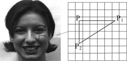
The relative positional relationship of points P, P₁ and P₂ in the Figure 1 can be described by the following formula. (9) $\left\{\begin{array}{l}x<x_1\text{, }y=y_1\\ x=x_2\text{, }y<y_2\end{array}\right.$(9) The formula (9) describes the numerical relationship of the abscissa and ordinate values of the constituent points P, P₁ and P₂, where the abscissa is from left to right, and the ordinate is from top to bottom. In addition to the numerical relationship of the abscissa and ordinate values in the figure, there are three other types. Therefore, according to the relative positions of the points forming the triangle, a total of 4 different right-angled triangles can be formed, as shown in Figure 2.

Figure 2. Schematic diagram of 4 right-angled triangle

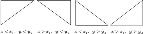
According to the schematic diagram, the 4 types of right-angled triangles are coded sequentially, which are 0, 1, 2, and 3 respectively.

Define the binary description function S(x): (10) $\text{S}\left(x\right)=\left\{\begin{array}{l}0\text{, }x<0\\ 1\text{, }x>0\end{array}\right.$(10) According to the 4 types of triangle vertex coordinates in formula (10) and Figure 2, the code of the above triangle can be calculated according to formula (11). (11) $\text{c}\left(\text{P},{\text{P}}_1,{\text{P}}_2\right)=\text{S}\left(x-x_1\right)+2\text{S}\left(y-y_2\right)$(11) In the same triangle type, 13 different triangles can be obtained according to the different gray values of the triangle vertices, as shown in Table 1.

Table 1. Table of vector triangle pattern

diagram	relationship	code	diagram	relationship	code
	$\text{I}<{\text{I}}_2<{\text{I}}_1$	−6		${\text{I}}_2<I={\text{I}}_1$	1
	$\text{I}<{\text{I}}_1<{\text{I}}_2$	−5		${\text{I}}_1<I<{\text{I}}_2$	2
	$\text{I}<{\text{I}}_1={\text{I}}_2$	−4		${\text{I}}_1<I={\text{I}}_2$	3
	$\text{I}={\text{I}}_2<{\text{I}}_1$	−3		${\text{I}}_1={\text{I}}_2<I$	4
	${\text{I}}_2<I<{\text{I}}_1$	−2		${\text{I}}_2<{\text{I}}_1<I$	5
	$\text{I}={\text{I}}_1<{\text{I}}_2$	−1		${\text{I}}_1<{\text{I}}_2<I$	6
	$\text{I}={\text{I}}_2={\text{I}}_1$	0

Similar to coding with 4 types of right-angled triangles, comparing I and I₁, there are 3 numerical relationships:, and comparing I and I₂, there are also 3 numerical relationships. Therefore, it is necessary to define a three-value description function ${\text{S}}_2\left(x\right)$: (12) ${\text{S}}_2\left(x\right)=\left\{\begin{array}{l}\begin{array}{c}-1\text{, }x<0\\ 0\text{, }x=0\end{array}\\ 1\text{, }x>0\end{array}\right.$(12) Combining the numerical relationship of I and I₁, I and I₂ can get a total of 9 results, respectively: (1) $\text{I}<{\text{I}}_1\text{and I}<{\text{I}}_2$, (2) $\text{I}<{\text{I}}_1\text{and I}={\text{I}}_2$, (3) $\text{I}〈{\text{I}}_1\text{and I}〉{\text{I}}_2$, (4) $\text{I}={\text{I}}_1\text{and I}<{\text{I}}_2$, (5) $\text{I}={\text{I}}_1\text{and I}={\text{I}}_2$, (6) $\text{I}={\text{I}}_1\text{and I}>{\text{I}}_2$, (7) $\text{I}>{\text{I}}_1\text{and I}<{\text{I}}_2$, (8) $\text{I}>{\text{I}}_1\text{and I}={\text{I}}_2$, (9) $\text{I}>{\text{I}}_1\text{and I}>{\text{I}}_2$. Also, because I₁ and I₂ also have 3 numerical relationships, among the 9 combined relationships, relationship (1) and relationship (9) can be further obtained by combining the 3 numerical relationships of I₁ and I₂. The results are (10) $\text{I}<{\text{I}}_1<{\text{I}}_2$, (11) $\text{I}<{\text{I}}_1={\text{I}}_2$, (12) $\text{I}<{\text{I}}_2<{\text{I}}_1$, (13) $\text{I}>{\text{I}}_1>{\text{I}}_2$, (14) $\text{I}>{\text{I}}_1={\text{I}}_2$, (15)$\text{I}>{\text{I}}_2>{\text{I}}_1$. The remaining 7 kinds of results plus the 6 kinds of results obtained, finally get the numerical relationship of I, I₁ and I₂, a total of 13 kinds, that is, the 13 kinds of numerical relationships described in Table 1. In order to make the program code more concise, we encode the vector triangle pattern from −6 to 6.

Through the numerical relationship of I, I₁ and I₂, the coding is arranged in the order in Table 1, and the coding results are 13 from −6 to 6. Combined with the three-value description function ${\text{S}}_2\left(x\right)$ of formula (12), the mathematical description after vector triangle coding is defined, as in formula (13). (13) $\begin{array}{rl}& \text{v}\left(\text{I},{\text{I}}_1,{\text{I}}_2\right)\\ & =\left(\begin{array}{c}3{\text{S}}_2\left(\text{I}-{\text{I}}_2\right)+{\text{S}}_2\left(\text{I}-{\text{I}}_1\right)+0.5{\text{S}}_2\left({\text{I}}_1-{\text{I}}_2\right)-1.5,\\ \text{I}<{\text{I}}_1,\text{I}<{\text{I}}_2\text{and }{\text{I}}_1\ne {\text{I}}_2\\ 3{\text{S}}_2\left(\text{I}-{\text{I}}_2\right)+{\text{S}}_2\left(\text{I}-{\text{I}}_1\right)+0.5{\text{S}}_2\left({\text{I}}_1-{\text{I}}_2\right)+1.5,\\ \text{I}>{\text{I}}_1,\text{I}>{\text{I}}_2\text{and }{\text{I}}_1\ne {\text{I}}_2\\ 3{\text{S}}_2\left(\text{I}-{\text{I}}_2\right)+{\text{S}}_2\left(\text{I}-{\text{I}}_1\right),\text{others}\end{array}\right)\end{array}$(13) In summary, a total of 52 (4×13) vector triangle patterns can be obtained. From formula (12) and formula (13), 52 vector triangle coding mathematical descriptions can be obtained, such as formula (14). (14) $\text{T}\left(\text{c},\text{v}\right)=13\text{c}\left(\text{P},{\text{P}}_1,{\text{P}}_2\right)+6+\text{v}\left(\text{I},{\text{I}}_1,{\text{I}}_2\right)$(14) The 52 kinds of vector triangle patterns describe the relationship between any three pixels in the image that meet the conditions of a right-angled triangle. When counting the number of vector triangles in the facial expression image, first fix the position of a pixel P, then determine the length relationship of multiple groups of different two right-angle sides, after that calculate the number according to the 52 kinds of vector triangle patterns to obtain the vector triangle statistics histogram H, where $\text{H}=\left\{{\text{H}}_0,{\text{H}}_1,{\text{H}}_2,\dots ,{\text{H}}_{51}\right\}$. The statistical method of ${\text{H}}_{\text{i}}$ is as in formula (15) and formula (16). (15) $\begin{array}{rl}{\text{H}}_{\text{i}}& =\sum _{\text{p}}\text{I}\left\{\text{T}\left(\text{c},\text{v}\right)=\text{i}\right\},\text{i}=0,1,2,\dots ,51\end{array}$(15) (16) $\begin{array}{rl}\text{I}\left\{\text{A}\right\}& =\left\{\begin{array}{l}0,Aisfalse\\ 1,Aistrue\end{array}\right.\end{array}$(16) Through the above method, the texture information between pixels in the facial expression image is counted according to the vector triangle pattern, and the counted number of vector triangles of different patterns is used as the facial expression feature.

3.2. Vector triangle scale and region selection

When extracting vector triangle features, we need to fix $\mathrm{\Delta }\text{x}$ and $\mathrm{\Delta }\text{y}$, that is, fix the length of the right-angle side of the right-angled triangle parallel to the abscissa and the length of the right-angle side parallel to the ordinate, and count the number of vector triangles at different scales. Different $\mathrm{\Delta }\text{x}$ and $\mathrm{\Delta }\text{y}$ reflect the texture feature information between different pixel distances. Figure 3 shows an example of the vector triangle scale mode.

Figure 3. Sample of vector triangle scale model

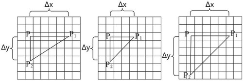
Different values of $\mathrm{\Delta }\text{x}$ and $\mathrm{\Delta }\text{y}$ correspond to a vector triangle scale, and the texture information of neighboring pixels obtained by counting the number of vector triangles in the facial expression image with different scales or combinations of different scales is also completely different. Every time a scale is selected, a 52-dimensional feature space can be obtained. Assuming that vector triangles of n kinds of scales or combinations of scales are counted, the statistical histogram of vector triangle patterns can be expressed in the form of formula (17). (17) $\text{H}=\left\{{\text{H}}_{1,0},\dots ,{\text{H}}_{1,51,}{\text{H}}_{2,0},\dots ,{\text{H}}_{\text{n},0},\dots ,{\text{H}}_{\text{n},51}\right\}$(17) Among them, each histogram in the statistical histogram represents the statistical quantity of the feature vector triangle pattern under a specific scale or combination of scales. Similar to formula (15), we can get the mathematical representation of each histogram, such as formula (18). (18) $\begin{array}{l}{\text{H}}_{\text{j},\text{i}}=\sum _{\text{p}}\sum _{\mathrm{\Delta }\text{x},\mathrm{\Delta }\text{y}}\text{I}\left\{{\text{T}}_{\mathrm{\Delta }\text{x},\mathrm{\Delta }\text{y}}\left(\text{c},\text{v}\right)=\text{i}\right\},\\ \text{i}=0,1,2,\dots ,51,\text{j}=1,2,\dots ,\text{n}\end{array}$(18) In summary, the dimension of the final extracted texture feature space is directly related to the number of selected scales or scale combinations. When n types of scales or scale combinations are selected, a texture feature matrix of 52×n can be obtained. Generally, in order to more completely represent the texture relationship between local pixels, vector triangles of multiple scales are selected for statistics. For example, there are 9 scale selection methods in a 3×3 pixel area, and there are 16 scale selection methods in a 4×4 pixel area, in addition to the use of a combination of multiple scales as statistical standards, which leads to the size of the feature space extracted during feature extraction is too large, under the premise of increasing the difficulty of optimization and recognition It is also easy to cause mixed information. Moreover, the extracted features can only describe the geometric information between adjacent pixels. If describe the pixels that are far away is needed, increase the scale is also necessary. Therefore, the texture feature extraction scheme selected in this paper adds a region extraction strategy to the vector triangle statistics combined with a single scale, which achieves the goal of extracting complete feature information with fewer scales through the combination of scales and regions. From the pixel level, the original facial expression picture is divided into multiple non-overlapping rectangular regions. The schematic diagram of the region division is shown in Figure 4.

Figure 4. Schematic diagram of image region division

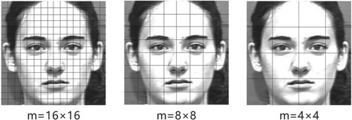
After dividing the facial expression image into several equal rectangular regions, all the pixels in the rectangular region are averaged according to formula (19), and the averaged value is used to represent the value of the rectangular region. (19) ${\text{I}}_{\text{m}}=\frac{1}{\text{m}}\sum _{\text{i}=1}^{\text{m}}{\text{I}}_{\text{i}}$(19)

Where m represents the number of pixels in the rectangular region, and I_i is the gray value of the i-th pixel in the rectangular region. Regarding the rectangular region as a whole, the set of pixel points is taken as the ‘point’ of the comparison vector triangle pattern, and the average value of the gray value of all points in the pixel point set is taken as the value corresponding to the ‘point’. As shown in Figure 4, there are 3 different region division methods. Select a single-scale combination to extract features, and the corresponding feature space will have 156 (3×52) dimensional feature values. At this time, the original vector triangle pattern with a smaller scale can be scaled by selecting different regions, and different scale combinations can be selected in different regions. The feature space can be selected more flexibly while ensuring that the feature space is not too large. So that the feature space can better describe the texture features of the image, and the regional averaging operation reduces the impact of individual pixel values when the interference changes, and improves the resistance of the feature space to interference.

The region division method selected in this paper is as follows: region 1, a single pixel is a region; region 2, a pixel in the adjacent 2×2 range is a region; region 3, a pixel in the adjacent 4×4 range is one Area, that is, starting from region 1, the pixels in the 2×2 range of the previous region are combined to become the next region division. The selection of specific scales in each region is discussed in Section 4.

In the task of facial expression recognition, high-dimensional features often have the following problems: too many features with weak characterization ability affect the accuracy of feature recognition; too large feature space affects the computational efficiency of feature classification. Therefore, the main purpose of feature optimization is to reduce the dimension of the feature space as much as possible on the premise that the feature space has enough information to support the classification task. In other words, it is to remove the redundancy in the original feature space, so that the feature space can more efficiently describe the relationship between the solution problem and the model.

In this paper we draw on the idea of feature selection in the decision tree, and regard each feature extracted as a decision, and the specific feature value is regarded as a decision option. Then the results that may appear in the data set, that is, the expression results we need to classify. Similar to the method of calculating the gain matrices (Chen et al. 2020), the information it contains can be represented by the concept of information entropy, and the calculation method is shown in formula (20). (20) $\text{H}\left(\text{D}\right)=-\sum _{\text{K}=1}^{\text{K}}\frac{|{\text{C}}_{\text{K}}|}{|\text{D}|}\log \frac{|{\text{C}}_{\text{K}}|}{|\text{D}|}$(20) Where K represents the number of labels of image classification in the data set, D represents the number of pictures in the data set, and ${\text{C}}_{\text{K}}$ represents the number of pictures of a specific label. We quantify the information contained in all pictures as information entropy H(D). From formula (20), it can be seen that the label with the smaller the probability of appearing in the data set, the more information it contains. On the contrary, the label with the larger the probability of appearing, the less information it contains.

When we choose to use a feature to divide the entire data set, the information entropy contained in the data will also change accordingly. The difference of the information entropy before and after the feature division can represent the information gain brought by using the feature to divide the data. Larger information gain can be understood as the ‘purity’ of the data set rises faster if the data set is divided by the feature value. Simply put, the feature is better in the data set. The calculation formula of information gain is as formula (21). (21) $\text{H}\left(\text{D},\text{A}\right)=\text{H}\left(\text{D}\right)-\text{H}\left(\text{D|A}\right)$(21) $\text{H}\left(\text{D|A}\right)$ is the information entropy of the data set divided by feature A, similar to formula (20), and can be obtained by formula (22) and formula (23). (22) $\begin{array}{rl}\text{H}\left(\text{D|A}\right)& =\sum _{\text{V}=1}^{\text{V}}\frac{|{\text{D}}_{\text{V}}|}{|\text{D}|}\text{H}\left({\text{D}}_{\text{V}}\right)\end{array}$(22) (23) $\begin{array}{rl}\text{H}\left({\text{D}}_{\text{V}}\right)& =-\sum _{\text{K}=1}^{\text{K}}\frac{|{\text{C}}_{\text{VK}}|}{|{\text{D}}_{\text{V}}|}\log \frac{|{\text{C}}_{\text{VK}}|}{|{\text{D}}_{\text{V}}|}\end{array}$(23) Among them, V represents different values of the feature, and $\text{H}\left({\text{D}}_{\text{V}}\right)$ represents the information entropy of the feature value at different values. In order to calculate $\text{H}\left({\text{D}}_{\text{V}}\right)$, it is necessary to calculate the number of pictures with different labels corresponding to different values of feature A, that is, ${\text{C}}_{\text{VK}}$. Therefore, the information entropy of the data set after the feature division can be calculated, and the information gain can be obtained.

However, the above method of calculating and calculating information gain has another drawback. When there are many feature values, that is, when the number of V is large, no matter what the value of V, the value of ${\text{C}}_{\text{VK}}$ will always be a small value, then $\text{H}\left({\text{D}}_{\text{V}}\right)$ will always be a large value, thus the calculated information gain cannot accurately express the quality of the feature. For facial expression image recognition tasks, most of the extracted feature values are continuous values. When calculating information entropy, it usually needs to be converted into discrete data segments. At this time, there are more possible values for features, and the above problems will occur. For this reason, we consider using the information gain rate to describe the representation ability of the feature value.

Compared with the information gain, the information gain rate adds a penalty parameter. The penalty parameter is smaller when the number of feature value is larger, the penalty parameter is larger when the number of feature value is smaller. The information gain rate is obtained through the product of the information gain and the penalty parameter, so as to alleviate the problem of inaccurate description caused by more number of feature value. The penalty parameter is as in formula (24). (24) $\text{P}=\frac{1}{{\text{H}}_{\text{A}}\left(\text{D}\right)}=\frac{1}{-{\sum }_{\text{i}=1}^{\text{n}}\frac{|{\text{D}}_{\text{i}}|}{|\text{D}|}{\log }_2\frac{|{\text{D}}_{\text{i}}|}{|\text{D}|}}$(24) Where ${\text{H}}_{\text{A}}\left(\text{D}\right)$ is the entropy of the random variable when the data set D is divided by the feature A. $|{\text{D}}_{\text{i}}|$ is the number of feature A in the data set whose value is ${\text{D}}_{\text{i}}$. That is, the penalty parameter is the reciprocal of the information entropy calculated after the data set D is divided according to the characteristics of the data set as a random variable.

The above methods for calculating the information gain rate are all realized on the basis of converting the extracted continuous facial expression feature values into discrete decision options. Different conversion methods directly affect the number of decision options. In this paper, we directly divide the value interval according to the intermediate value of adjacent values, and convert continuous feature values into discrete feature options. Experimental results show that this direct conversion method is convenient for calculation and has good results. Specific steps are as follows:

1. The initial value interval is $\left(-\mathrm{\infty },\mathrm{\infty }\right)$. Calculate the intermediate value ${\text{a}}_{\text{n}}$ for the next two continuous feature values ${\text{f}}_0\text{and }{\text{f}}_1$, and insert the intermediate value ${\text{a}}_{\text{n}}$ into the value interval.

2. Calculate the intermediate values ${\text{a}}_{\text{n}}$ and ${\text{b}}_{\text{n}}$ for the following continuous feature value ${\text{f}}_{\text{n}+1}$ and the two ends of the value interval.

3. Determine whether the difference between ${\text{a}}_{\text{n}}$ and the two ends of the current value interval is bigger than the threshold $\rho$, if yes, insert the intermediate value ${\text{a}}_{\text{n}}$ into the value interval, if not, do nothing.

4. Determine whether the difference between ${\text{b}}_{\text{n}}$ and the two ends of the current value interval is greater than the threshold $\rho$ if yes, insert the intermediate value ${\text{b}}_{\text{n}}$ into the value interval, if not, do nothing.

5. Iterative calculation, if the traversal of continuous feature value has not been completed, skip to step (2).

Finally, continuous feature values are transformed into discrete decision options through the divided value interval, and the threshold $\rho$ selected in this paper is ${10}^{-6}$.

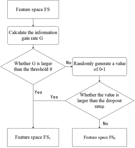
After obtaining the high-dimensional feature space and the information gain rate corresponding to each feature through the above method, feature selection is required. The most common feature selection strategy is threshold selection. Assuming that the threshold for feature selection by the information gain rate is $\theta$, then the original feature space can be divided into two sets, as shown in formula (25). (25) $\text{FS}=\text{F}{\text{S}}_1+\text{F}{\text{S}}_0$(25) Among them, FS₁ is the selected feature, the information gain rate corresponding to each feature in FS₁ is bigger than or equal to the threshold $\theta$, FS₀ is the unselected feature, and the information gain rate corresponding to each feature in FS₀ is smaller than the threshold $\theta$, and the collection of the set FS₁ and the set FS₀ is the feature space FS.

Threshold selection can filter out most of the features with poor characterization ability, but it will also bring corresponding problems. For example, when the feature space is reduced through the threshold selection strategy, in order to improve the feature space representation ability, a larger threshold is often used, which will also make the generalization ability of the feature space poor, resulting in the problem of overfitting. Moreover, the information gain rate of the features in this paper has a small gap within the optimal threshold range, and it is difficult to avoid overfitting only by the method of threshold selection. Therefore, this paper adds a random dropout strategy to the threshold selection strategy.

The random dropout strategy was originally a strategy used in machine learning to effectively alleviate the occurrence of overfitting Salehinejad and Valaee (2019). The basic principle is to hide some neurons randomly during the propagation of neural network neurons to make the model's generalization ability stronger and will not rely too much on dictating local features. In this paper, referring to the application of random dropout strategy in neural networks, when the feature is selected by the threshold, it is not simply based on the threshold to simply delete the features whose information gain rate is smaller than the threshold from the feature space, but based on the random dropout rate $\mu$, the features whose information gain rate is smaller than the threshold are discarded. Figure 5 shows the basic steps of using threshold selection strategy and random dropout strategy for feature selection. The specific selection threshold and random discard rate are determined by experiments, see section 4 for details.

Figure 5. Basic steps of feature selection results

4. Experiment

4.1. Experimental data and platform

The experiment in this paper starts with the opposite expression unit of positive expression and negative expression, using The Extended Cohn-Kanade (CK+) data set. 3589 images were selected as the training set, including 1668 positive expression images (mainly labeled as happy or surprised) and 1921 negative expression images (mainly labeled as disgust, fear, and sadness). Selected 1301 images as the test set, including 664 positive expression images and 637 negative expression images. Table 2 shows the details.

Table 2. Table of experimental data

	Train set	Test set
positive	1668	664
negative	1921	637
all	3589	1301

The experimental platform of this paper is windows7, and the development environment includes Python3.6 and matlab2016. The hardware configuration of this experiment is Intel corei7-9700 K, 8-core 16-wire, 3.60 GHz, 48GB memory, NVIDIA GTX2080 8G graphics card.

4.2. Similarity evaluation criteria

The purpose in the stage of feature selection is to improve the characterization ability of the feature space, so that it can distinguish between positive and negative samples and have similarity when facing similar samples. In the feature selection method based on the information gain rate as described above, it is necessary to select an appropriate selection threshold and dropout rate to improve the characterization ability of the feature space under the premise of ensuring the diversity of features. Therefore, at this stage, this paper uses Pearson Correlation Coefficient and Tanimoto Coefficient to describe the similarity between sample features. The calculation method of Pearson's correlation coefficient is shown in formula (26). (26) $\text{r}=\frac{{\sum }_{\text{i}=1}^{\text{n}}\left({\text{X}}_{\text{i}}-\overline{\text{X}}\right)\left({\text{Y}}_{\text{i}}-\overline{\text{Y}}\right))}{\sqrt{{\sum }_{\text{i}=1}^{\text{n}}{\left({\text{X}}_{\text{i}}-\overline{\text{X}}\right)}^2}\sqrt{{\sum }_{\text{i}=1}^{\text{n}}{\left({\text{Y}}_{\text{i}}-\overline{\text{Y}}\right)}^2}}$(26) Where r represents the Pearson Correlation Coefficient, and $\overline{\text{X}}$ and $\overline{\text{Y}}$ are the sample averages of the variables X and Y, respectively. The value range of Pearson Correlation Coefficient is between [−1, 1. When the value is 0, it means that the two variables are not correlated. When the value is −1 or 1, it means that the two variables are strongly correlated. The value of −1 shows a negative correlation, and the value of 1 shows a positive correlation.

The calculation method of Tanimoto Coefficient is shown in formula (27). (27) $\text{T}\left(\text{X},\text{Y}\right)=\frac{\text{X}\cdot \text{Y}}{{||\text{X}||}^2+{||\text{y}||}^2-\text{X}\cdot \text{Y}}$(27) Where $\text{X}\cdot \text{Y}$ represents the product of the sample vector, and ${\text{X}}^2=\sqrt{\sum _{\text{i}=1}^{\text{n}}{\text{X}}_{\text{i}}}$ represents the modulus of the vector. The larger the value, the higher the similarity of the samples.

4.3. Experimental results and analysis

In order to explore the best vector triangle feature extraction scales under different region division modes, this paper randomly selects 200 groups of similar samples (between 100 groups of positive expression images and 100 groups of negative expression images) and 200 groups of positive and negative under different region division modes from CK+ data set. Samples extracted vector triangle texture features of different scales, and calculated the Pearson Correlation Coefficient between samples of the same type and between positive and negative samples.

As shown in Table 3, it is the average Pearson Correlation Coefficient between the vector triangle texture features extracted at different scales between the similar samples under the division of region 1. Among them, the rows in the table indicate the pixel values of the vector triangle scale on the Y axis, and the columns indicate the pixel values on the X axis. For example, the first row and the second column indicate that the vector triangle scale is selected as $\mathrm{\Delta }\text{x}=2\text{, }\mathrm{\Delta }\text{y}=1$. At this time, the average Pearson Correlation Coefficient between 200 groups of similar samples under the division of area 1 is 0.028532.

Table 3. Table of Pearson Correlation Coefficient of the same sample at different scales in region 1

X/Y	1	2	3	4	5
1	0.013733	0.028532	0.027642	0.045692	0.031781
2	0.010283	0.009076	0.038918	0.062623	0.077319
3	0.019125	0.044253	0.066344	0.089632	0.087257
4	0.041662	0.058973	0.102010	0.112845	0.153321
5	0.051835	0.074214	0.126495	0.151254	0.189170

The same processing is done for the positive and negative samples, and the average Pearson Correlation Coefficient between the vector triangle texture features extracted at different scales between the positive and negative samples under the division of region 1 is obtained. As shown in Table 4.

Table 4. Table of Pearson Correlation Coefficient of the positive and negative samples at different scales in region 1

X/Y	1	2	3	4	5
1	0.015317	0.01646	0.026948	0.022446	0.03602
2	0.006791	0.014646	0.024425	0.05305	0.05772
3	0.020751	0.033688	0.044006	0.078128	0.077317
4	0.027245	0.067109	0.086031	0.070522	0.144535
5	0.065349	0.054434	0.131504	0.136674	0.204841

For the final classification task, in the most ideal feature space, the features of similar samples should be as similar as possible, that is, the larger the average Pearson Correlation Coefficient between similar samples, the better. And the features between positive and negative samples should be more different, that is, the smaller the average Pearson Correlation Coefficient between positive and negative samples, the better. Therefore, this paper uses the difference of the average Pearson Correlation Coefficient between the similar sample and the positive and negative samples to describe the quality of the vector triangle texture features extracted with different scales in the current regional mode.

Figure 6 shows the three dimensional effect diagram of the difference in the average Pearson Correlation Coefficient between the similar sample and the positive and negative samples at different scales in area 1.

Figure 6. Three-dimensional rendering of average Pearson Correlation Coefficient difference in region 1

The X axis and Y axis value changes correspond to the $\mathrm{\Delta }\text{x}$ and $\mathrm{\Delta }\text{y}$ selected by the vector triangle scale, and the Z axis value represents the difference of the average Pearson Correlation Coefficient. It can be found that when x=4 and y=4, the average Pearson Correlation Coefficient difference reaches the highest peak, so under the division of region 1, the best scale is $\mathrm{\Delta }\text{x}=4\text{, }\mathrm{\Delta }\text{y}=4$.

In the same way, in order to explore the best scale selection under the division of region 2 and region 3, this paper calculates the average Pearson Correlation Coefficient of vector triangle texture features between similar samples and the positive and negative samples under the division of region 2 and region 3. The results are shown in Figures 7–8.

Figure 7. Three-dimensional rendering of average Pearson Correlation Coefficient difference in region 2

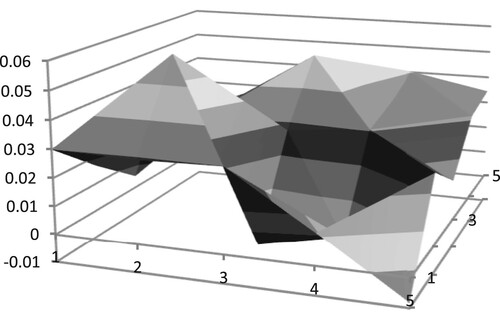
Figure 8. Three-dimensional rendering of average Pearson Correlation Coefficient difference in region 3

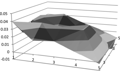
Among them, when x=2 and y=2, the average Pearson Correlation Coefficient difference reaches the highest peak, so under the division of region 2, the best scale is $\mathrm{\Delta }\text{x}=2\text{, }\mathrm{\Delta }\text{y}=2$.

Among them, when x=1 and y=1, the average Pearson Correlation Coefficient difference reaches the highest peak, so under the division of region 3, the best scale is $\mathrm{\Delta }\text{x}=1\text{, }\mathrm{\Delta }\text{y}=1$.

After determining the area division method and the selection of the vector triangle scale, it is necessary to explore the optimal selection threshold and random dropout rate in the feature optimization stage according to the information gain rate of the feature. According to the description in Section 3, this paper calculates the information gain rate of the feature space, and calculates the difference between the positive and negative samples and the average Pearson Correlation Coefficient and the average Tanimoto Coefficient before and after optimization of the positive and negative samples and similar samples according to different selection thresholds and random dropout rates.

Table 5 shows the results of the positive and negative sample experiment, where the selection threshold is from 0.175–0.100, the span is 0.025, and the random dropout rate is 0.7 or 0.5.

Table 5. Experimental results of positive and negative samples

Select threshold	Dropout rate	Pearson correlation coefficient difference	Tanimoto coefficient difference
0.175	0.7	0.037196	0.029084
0.175	0.5	0.026052	0.014121
0.150	0.7	0.059815	0.033724
0.150	0.5	0.026140	0.013311
0.125	0.7	0.078500	0.029157
0.125	0.5	0.037192	0.013056
0.100	0.7	0.082734	0.015023
0.100	0.5	0.034848	0.006604

In the positive and negative samples, the similarity between the ideal features should be low. In this case, the smaller the correlation, the better. That is, the Pearson Correlation Coefficient is close to −1, and the Tanimoto Coefficient is close to 0. In order to better describe the changes in the feature space before and after optimization, this paper uses the correlation before optimization minus the correlation after optimization when processing positive and negative samples, and uses the difference in correlation to describe the optimization effect. The greater the difference, the optimization effect the better.

The three sets of data with the largest average Pearson Correlation Coefficient difference are selected as the 3rd, 5th, and 7th rows, and the three sets of data with the largest average Tanimoto Coefficient difference are selected as the 1st, 3rd, and 5th rows. Comprehensively compare the difference between Pearson Correlation Coefficient and Tanimoto Coefficient, the selection threshold and random dropout rate used in the 3rd and 5th rows are the optimal solutions between positive and negative samples. That is, the selection threshold is 0.150, the random dropout rate is 0.7, and the selection threshold is 0.125, and the random dropout rate is 0.7.

Similar to the positive and negative sample experiments, Table 6 shows the experimental results of similar samples. The difference from the experiment of the positive and negative sample group is that the similarity between the ideal features in the same sample is higher. At this time, the larger the correlation, the better, that is, the Pearson Correlation Coefficient and the Tanimoto Coefficient are both close to 1. So, this paper uses the correlation degree after optimization minus the correlation degree before optimization to describe the optimization effect. The larger the difference, the better the optimization effect. The three sets of data with the largest average Pearson Correlation Coefficient difference are selected as the 3rd, 5th, and 7th rows, and the three sets of data with the largest average Tanimoto Coefficient difference are selected as the 1st, 3rd, and 5th rows. Comprehensively compare the difference between Pearson Correlation Coefficient and Tanimoto Coefficient, the selection threshold and random dropout rate used in the 3rd and 5th rows are the best solutions among similar samples. That is, the selection threshold is 0.150, the random dropout rate is 0.7, and the selection threshold is 0.125, and the random dropout rate is 0.7.

Table 6. Experimental results of similar samples

Select threshold	Dropout rate	Pearson correlation coefficient difference	Tanimoto coefficient difference
0.175	0.7	0.046481	0.039295
0.175	0.5	0.010432	0.009685
0.150	0.7	0.060255	0.034169
0.150	0.5	0.019860	0.009933
0.125	0.7	0.081274	0.024763
0.125	0.5	0.038695	0.014688
0.100	0.7	0.076061	0.016102
0.100	0.5	0.038679	0.004919

In summary, when feature optimization is performed, the selection threshold is 0.150, the random dropout rate is 0.7, and the selection threshold is 0.125, and the random dropout rate is 0.7 as the optimal solution. But comparing another set of choices, when the selection threshold is 0.150 and the random dropout rate is 0.7, the number of features in the feature space is too small, and the generalization ability of the feature space cannot be guaranteed. This is contrary to the original intention of using the random dropout strategy, so this paper chooses the threshold value is 0.125, and the random dropout rate is 0.7 as the parameters for feature optimization.

After obtaining the feature space, according to the description in Section 2, the WSC algorithm is used for facial expression recognition. The result is shown in Figure 9.

Figure 9. Expression recognition result graph based WSC

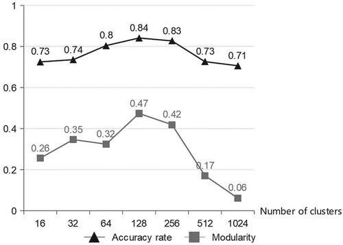
The abscissa indicates that the number of clusters of hierarchical clustering during re-annotation is 16(2⁴), 32(2⁵), 64(2⁶), 128(2⁷), 256(2⁸), 512(2⁹), 1024(2¹⁰), from left to right, the triangle represents the accuracy of the classification result and the true label, and the square represents the clustering modularity corresponding to the number of clusters. The weakly annotated facial expression data is obtained by inverting the real label according to a specific ratio. The graphic experiment is carried out under the condition of the weak annotation accuracy rate of 0.7, that is, the label data with a ratio of 0.3 is inverted.

When the number of clusters is 128(2⁷), the modularity reaches the maximum, and within the range of 0.3–0.7, the clustering effect is good. At this time, the accuracy of the classification result of the WSC algorithm is 0.84, which is also the highest accuracy for different clustering numbers. And observe the change trend of accuracy rate broken line and the change trend of modularity, the two trends are very similar. Therefore, modularity can be used as an index to determine the number of clusters in hierarchical clustering in the re-annotation stage, that is, select the number of clusters which the modularity is the largest.

Observing the changing trend of the accuracy rate and modularity, both increase first and then decrease, that is, when the number of clusters is too much or too few, the accuracy and modularity are both low. Analyze the steps of the re-annotation algorithm. When the number of clusters is too small, several large clusters are often formed when clustering weak annotation data, and some data in the large clusters that are classified into one category due to subtle differences cannot be correct. Therefore, when the number of clusters is too small, the accuracy is often not high. When the number of clusters is too large, there will be many small clusters in the result of clustering weakly annotated data, that is, the number of sample points in the cluster is too small, and there may be only one or two samples. In this case, use voting to improve the effect of label data is not very obvious, so the accuracy rate is also close to the selected weak annotation accuracy rate of 0.7.

Table 7 shows the comparison with the recognition results of other methods. UD means using Unannotated Data, PN means Pruning Noisy annotation, and rows 1st, 2nd and 3rd are the experimental results of classifying using Fuzzy C-Means Clustering (FCM), Fuzzy Inference System (FIS) and Support Vector Machine (SVM), respectively. The 4th row uses the WSC algorithm to classify the unoptimized feature space, and the 5th row is the experimental result of classifying the optimized feature space. The above experiments are all carried out on the weak annotation data set with a weak annotation rate of 0.7, that is, the annotation accuracy rate is 0.7.

Table 7. Table of different methods results

Classifier or feature method	Accuracy rate	UD	PN
FCM Liliana et al. (2018)	80.71%	✓	✗
FIS Liliana et al. (2018)	72.0%	✓	✗
SVM Melacci and Belkin (2011)	93.1%	✗	✗
Unoptimized features	78.3%	✓	✓
ours	84.1%	✓	✓

Both FCM and FIS directly use the coordinates of the face points, instead of transforming the coordinates of the face points into realistic expression features as in this paper. Although it is possible to use unannotated data for semi-supervised learning, it is impossible to modify the erroneous noise data in the data. In addition, the accuracy of our facial expression recognition scheme is still better than these two methods. The advantage of using the fuzzy method is that because the nature of facial expressions is fuzzy, the fuzzy method can tolerate the input conditions and produce the best recognition results. The biggest difference between this method and our method is the difference in input. Our method uses multi-scale and multi-region vector triangle texture features. Compared with the direct use of face pixels, it greatly reduces the processing of pixels that are irrelevant to emotional expression and improves the efficiency of the framework. SVM is recognized as an effective algorithm in pattern recognition and facial expression recognition, and has a high recognition rate. However, the fully annotated data must be used and the noise data cannot be modified.

In order to verify the experimental conclusions of the selection threshold and the random dropout rate, this paper classifies the feature spaces obtained under different selection thresholds and random dropout rates, and calculates the accuracy of facial expression recognition. The results are shown in Table 8.

Table 8. Table of feature optimization verification Experimental results

Select threshold	Dropout rate	Accuracy rate
0.175	0.7	0.833
0.150	0.7	0.839
0.125	0.7	0.841
0.100	0.7	0.787

When the selection threshold is 0.150, the random dropout rate is 0.7, and when the selection threshold is 0.125, the random dropout rate is 0.7, the recognition accuracy is higher, which is consistent with the results discussed in the previous experiment. And when the selection threshold is 0.125 and the random dropout rate is 0.7, the recognition accuracy is the highest.

In addition to the above experiments, in order to verify the versatility of the facial expression recognition scheme in this paper, we also use the expression images of the JAFFE data set and the Oulu-CASIA data set to conduct experiments. The JAFFE data set contains 7 expressions from Japanese female students, and the Oulu-CASIA data set contains 6 typical expressions under the imaging system of near-infrared light and visible light. This paper only uses expression images under visible light imaging conditions. The positive expression images and negative expression images of the JAFFE data set and Oulu-CASIA data set are identified using the WSC algorithm model trained by CK+ image, and compared and analyzed with other methods. The experimental results are shown in Table 9.

Table 9. Table of different data sets experimental results

Data set	Classification	Accuracy rate	UD	PN
JAFFE	FERF (Liliana and Basaruddin (2020))	82.0%	Π	Ο
	ISR (Liu et al. (2017))	83.5%	Ο	Ο
	ours	82.5%	Π	Π
Oulu-CASIA	Atlases (Guo et al. (2012))	75.5%	Π	Ο
	PPDN (Zhao et al. (2016))	84.6%	Ο	Ο
	ours	82.7%	Π	Π

It can be seen from Table 9 that the method in this paper can have a good recognition rate in both the JAFFE data set and the Oulu-CASIA data set, and can process unannotated data and pruning noisy annotation.

5 Conclusion

Aiming at the weakly supervised clustering algorithm that can use weak annotation data for facial expression recognition, this paper proposes a multi-scale and multi-region vector triangle texture feature extraction scheme, and based on the information gain rate combined with the strategy of threshold selection and random dropout to carry out the feature space Optimization. The experimental results show that, the feature extraction and optimization schemes in this paper are effective in the WSC algorithm, and the recognition accuracy after optimization is improved by 5.8%. And compared with traditional facial expression recognition schemes, it not only has a higher accuracy rate, but also has more usage scenarios (Handling weak annotation data). In addition, this paper also explores the optimal scale selection in the feature extraction stage and the optimal selection threshold and random dropout rate in the feature optimization stage through experiments, which have been verified in the recognition stage. Finally, facial expression image data that is different from the training and test data set is used to verify the generalization ability of the proposed scheme.

At present, the expression recognition scheme in this paper is still inadequate, and WSC algorithms often perform poorly when dealing with multi-label problems. Subsequent research will extend the scheme of this paper to more expression units, and then further realize the multi-label classification problem. In addition, it is also necessary to consider the randomly occurring uncertainties and stability in the optimization stage (Li & Liang, 2020; Zhao et al., 2020), increase stability analysis (Zou et al., 2021), and further improve the optimization effect of the feature space.

Acknowledgments

This work is supported by National Natural Science Foundation of China (No. 61873082), the ZheJiang province Natural Science Foundation of China (Nos. LY20F020022), and the National Key R&D Program of China (No. 2018YFB0204003), Basic Public Welfare Research Project of Zhejiang Province in China (No. LGG18F030002).

Disclosure statement

No potential conflict of interest was reported by the author(s).

Additional information

Funding

This work was supported by National Natural Science Foundation of China: [Grant Number No.61873082]; ZheJiang Provincial  Natural Science Foundation of China: [Grant Number No.LY20F020022]; Basic Public Welfare Research Project of Zhejiang Province in China: [Grant Number No. LGG18F030002]; National Key R&D Program of China: [Grant Number No. 2018YFB0204003].

References

- Barman, A., & Dutta, P. (2019). Influence of shape and texture features on facial expression recognition[J. IET Image Processing, 13(8), 1349–1363. https://doi.org/https://doi.org/10.1049/iet-ipr.2018.5481
- Caifeng, S., Shaogang, G., & Peter, W. M. (2005, September 14–14). Robust facial expression recognition using local binary patterns[C. IEEE International Conference on image processing. 370–373. https://doi.org/https://doi.org/10.1109/ICIP.2005.1530069
- Chen, Yun, Chen, Zhangping, Chen, Zhenyu, & Xue, Anke. (2020). Observer-based passive control of non-homogeneous Markov jump systems with random communication delays. International Journal of Systems Science, 51(6), 1133–1147. https://doi.org/https://doi.org/10.1080/00207721.2020.1752844
- Cheng-Dong, W. U., Zi-Wei, L. U., & Xiao-Sheng, Y. U. (2019). Image super resolution reconstruction algorithm based on weighted random forest. Control and decision. Control and Decision, 34(10), 2243–2248. https://doi.org/https://doi.org/10.13195/j.kzyjc.2018.0140
- Ghahari, A., Fatmehsari Y. R., & Zoroofi R. A. (2009, September 12–14). A novel clustering-based feature extraction method for an automatic facial expression analysis system[C//. International Conference on intelligent information hiding & multimedia signal processing, IEEE. https://doi.org/https://doi.org/10.1109/IIH-MSP.2009.38
- Gu, W., Cheng, X., Venkatesh, Y. V., Huang, D., & Lin, H. (2012). Facial expression recognition using radial encoding of local Gabor features and classifier synthesis. Pattern Recognition, 45(1), 80–91. https://doi.org/https://doi.org/10.1016/j.patcog.2011.05.006
- Guo, Y., Zhao, G., & Pietikäinen, M. (2012). Dynamic Facial Expression Recognition Using Longitudinal Facial Expression Atlases[M// Computer Vision – ECCV 2012. Springer Berlin Heidelberg, 2012.
- He, J. (2015). Research on extraction of facial expression features and hierarchical classification [D. Hefei University of Technology.
- Hong, B., & Tao, M. (2014, September 11–13). Feature extraction and facial expression recognition based on bezier curve[C//. IEEE International Conference on computer & information technology. IEEE. https://doi.org/https://doi.org/10.1109/CIT.2014.140
- Kubicek, B., Gupta A, S., & Kirsteins, I. (2020). Sonar target representation using two-dimensional Gabor wavelet features. The Journal of the Acoustical Society of America, 148(4), 2061–2072. https://doi.org/https://doi.org/10.1121/10.0002168
- Li, Qiang, & Liang, Jinling. (2020). Dissipativity of the stochastic Markovian switching CVNNs with randomly occurring uncertainties and general uncertain transition rates. International Journal of Systems Science, 51(6), 1102–1118. https://doi.org/https://doi.org/10.1080/00207721.2020.1752418
- Liliana D. Y., & Basaruddin, T. (2020, November 12–14). The fuzzy emotion recognition framework using semantic-linguistic facial features[C//. 2019 IEEE R10 humanitarian Technology Conference (R10-HTC)(47129). IEEE. https://doi.org/https://doi.org/10.1109/R10-HTC47129.2019.9042442
- Liliana D. Y., Widyanto M. R., & Basaruddin, T. (2018, October 27–28). Geometric facial components feature extraction for facial expression recognition[C. 2018 International Conference on advanced Computer science and information systems (ICACSIS). https://doi.org/https://doi.org/10.1109/ICACSIS.2018.8618248
- Liu, S., Li, L., Peng, Y., Qiu, G., & Tao, L. (2017). Improved sparse representation method for image classification. Iet Computer Vision, 11(4), 319–330. https://doi.org/https://doi.org/10.1049/iet-cvi.2016.0186
- Melacci, S., & Belkin, M. (2011). Laplacian support vector machines trained in the primal. Journal of Machine Learning Research, 12(3), 1149–1184.
- Meng, X., Xie, R., Jia, H., & Li, H. (2019). Identification of light Oil in 2D NMR spectra of tight sandstone reservoirs by using L1/L2 Two-parameter regularization. Energy & Fuels, 33(11), 10537–10546. https://doi.org/https://doi.org/10.1021/acs.energyfuels.9b02114
- Salehinejad, H., & Valaee, S. (2019, May 12–17). Ising-dropout: a regularization method for training and compression of deep neural networks[C//. ICASSP 2019-2019 IEEE International Conference on Acoustics, Speech and Signal Processing (ICASSP), Brighton, UK. https://doi.org/https://doi.org/10.1109/ICASSP.2019.8682914
- Zhao, K., Chu W. S., & Martinez, A. M. (2018, June 18–23). Learning facial action units from Web images with scalable weakly supervised clustering[C// 2018. IEEE/CVF Conference on Computer Vision and pattern recognition. IEEE. https://doi.org/https://doi.org/10.1109/CVPR.2018.00223
- Zhao, X., Liang, X., Liu, L., Li, T., Han, Y., Vasconcelos, N., & Yan, S. (2016, October 11–14). Peak-Piloted deep network for facial expression recognition[C//. European Conference on Computer vision, Springer, Cham. https://doi.org/https://doi.org/10.1007/978-3-319-46475-6_27
- Zhao, Zhongyi, Wang, Zidong, Zou, Lei, & Guo, Jiyue. (2020). Set-membership filtering for time-varying complex networks with uniform quantisations over randomly delayed redundant channels. International Journal of Systems Science, 51(16), 3364–3377. https://doi.org/https://doi.org/10.1080/00207721.2020.1814898
- Zheng, Z., Zheng, Z., & Tiantian, Y. (2010). Facial expression recognition based on Two-dimensional multi-scale Local Gabor Binary Pattern features. Journal of Computer Applications, 30(4), 964–966. https://doi.org/https://doi.org/10.3724/SP.J.1087.2010.00964
- Zhu, C., Wen, F., & Sun, J. (2011). A rank-order distance based clustering algorithm for face tagging[C// CVPR 2011. IEEE, 2011.
- Zhuo, K., Yang, Z., Yan, G., Yu, K., & Guo, W. (2019). An efficient graph clustering algorithm in signed graph based on modularity maximization. International Journal of Modern Physics C, 30(11), 1950095. https://doi.org/https://doi.org/10.1142/S0129183119500955
- Zou, Lei, Wang, Zidong, Hu, Jun, Liu, Yurong, & Liu, Xiaohui. (2021). Communication-protocol-based analysis and synthesis of networked systems: progress, prospects and challenges. International Journal of Systems Science, 1–22. https://doi.org/https://doi.org/10.1080/00207721.2021.1917721