Multi-layer Gaussian Mixture Model algorithm and its application in lithology classification

Abstract

Even in the same block, the difference in lithology distribution is small, but there is still a big difference in the distribution of the central wells and the edge wells in the block at the same level of depth. This is because we need to find data points of the same stratum depth instead of being disturbed by data points of horizontal depths. According to this problem, we propose two GMM algorithms based on EM: multi-layer GMM and two-layer GMM. The feature of multi-layer GMM is that even if there are edge wells far away from the exploratory well, this algorithm can still filter out data points that are not in the same formation depth through continuous averaging of initialization information in order to achieve a better effect of accurately predicting the lithology distribution of the stratum. Moreover, the robustness is more suitable for the general situation. In addition, in the blocks with relatively concentrated wells, we also propose a two-layer GMM method complementary. Compared with the multi-layer structure, due to the parallel structure, it is faster but less robust. The simulation results show that the multi-layer GMM algorithm proposed in this paper is compared with the multi-resolution clustering method based on graph theory, single-layer GMM and double-layer GMM. This algorithm achieves a better clustering effect than other methods.

Index Terms:

• Log interpretation
• lithology identification
• Gaussian Mixture Model
• clustering
• log response characteristics

I. Introduction

With the further increasing in the exploration and development of international oil and gas fields, the lithology of the reservoirs facing them has become more complicated, such as deep igneous rock reservoirs, tight limestone reservoirs, oil shale reservoirs, shale gas reservoirs and sandstone reservoirs, etc (Liu (2005); Tan and Zhao (2006); Tan and Zhang (2010); Huang et al. (2011); Zhang (2012); Hao et al. (2012); Shen et al. (2012); Wu et al. (2013)). As one of the major data sources of underground rock information, geophysical logging data has become increasingly significant in the interpretation of stratigraphic lithology on account of its high vertical resolution, good continuity and convenient acquisition Wang and Guo (2000). Lithology interpretation on the basis of logging data is the basis for ‘subsequent reservoir parameter calculations’, ‘oil and gas evaluations’ and also provides a basis for geological research such as ‘formation rhythm feature analysis’, ‘sedimentary facies division’ and ‘sedimentary environment analysis’.

On the basis of analyzing logging response characteristics, mathematical algorithms are introduced to solve the problem (Hu et al. (2015); Mou et al. (2015)), An, P., et al. An and Cao (2018) have studied the use of deep learning to divide 9 types of lithology, including sandstone, mudstone, carbonate and so on. Good results have been achieved. Cluster analysis is one of the very important algorithms for data mining. Since it has been proposed as a logging curve analysis tool An and Cao (2018), domestic and foreign researchers have also carried out some work on this. Tian, Y., et al. Tian et al. (2016) have used clustering methods. Lithofacies prediction has been carried out in the carbonate intra-platform gas field in the right bank of the Amu Darya Basin. Shi, X. L., et al. Shi et al. (2018) have determined the corresponding relationship between the logging facies and the rock facies in reference to the logging facies constraint. Moreover Shi has established the permeability evaluation model in accordance with the logging facies constraint. Bergamaschi, S., Ferreira, FJF., et al. Bergamaschi and Pereira (2001), Ferreira et al. (2010) have identified the lithology of non-core intervals with the aid of interpretation gamma ray logging. Gamma-ray logging has been performed well in correlation and sequence stratigraphy in the Ponta Grossa formation of the Devonian Basin in Parana, Brazil. Now it has become the most extensive lithology identifications method in the area. Identifying lithology in logging is founded on relevant principles that logging response and path lithology changes. However, no logging curve can clearly distinguish lithology. For example, the radioactivity of bentonite clay is lower than that of sandstone Dypvik and Eriksenf (1983). Other researchers have attempted to combine the extensive prior knowledge acquired for years with the study of fossils, sediments and gamma ray records in ‘sequence stratigraphy’ or ‘sedimentary and paleoenvironmental processes’ (Carelli and Borghi (2011); Grahn et al. (2013); Grahn et al. (2013)).

Cluster analysis involves the use of clustering algorithms to divide a set of logging data into electrical facies element, which is defined as ‘A set of logging responses that characterize sediments and we can distinguish them from other sediments.’ They can be displayed as inferred lithology profiles to help perform sequence stratigraphy and correlation Ye and Rabiller (2005). The usual clustering methods include ‘K-means clustering algorithm’ (K-means) Selim and Ismail (1984), ‘Ascendent Hierarchical Clustering’ (AHC) Johnson (1967), ‘Self-Organizing Map’ (SOM) Kohonen (1990) and ‘Multi-Resolution Clustering model based on Graph theory’ (MRGC) Kohonen (1990). Among them, the MRGC method performs best in the lithofacies clustering problem in the formation Ye and Rabiller (2000), Rahsepar et al. (2016). It is a multi-dimensional point pattern recognition method based upon non-parametric K nearest neighbors and graphical data representation. It can form natural data groups that may have different densities, sizes, shapes and relative intervals by analyzing the underlying structure of the data. This method can automatically determine the optimal number of clusters. But for special areas, such as low-permeability areas, it is impossible to obtain more detailed and accurate formation information. Since in block wells we need to infer the oil storage of the formation on the basis of various lithologies. This makes observing the distribution of lithologies in the formation that become an important link. However, due to the discontinuity and non-uniformity of the formation, we need to probe the formation in advance to artificially determine the parameter thresholds of the target well section to eliminate outliers impact when we cluster the lithology distribution of each well. That is to say, the problem greatly increases the difficulty of the work because we need to re-measure other wells in the block except exploratory wells.

Gaussian Mixture Model (GMM) Reynolds (2009) is a clustering method based on probability distribution. Not only can it make the classification of categories more non-linear, but it can also mine more important information from the data. But because this method is susceptible to outliers owing to its poor robustness. We randomly select exploratory wells in the block as initialization wells. Afterwards, we use the prior knowledge obtained from exploratory wells as initialization weights to pass to the next layer of GMM. Then the information generated by this layer and the information of the previous layer are averaged as the initialization weight and sent to the next layer of GMM. This not only makes use of the soft clustering characteristics of GMM to obtain a more detailed classification, but also increases the robustness of the model by connecting multiple single-layer GMM models in series. This method makes it possible to enjoy the benefits of mean initialization in the block even at the edge of the well and the classification will not cause the clustering to ‘deviate’ due to the interference of outliers. In view of the situation that the random exploratory wells are known and the exploratory wells are not at the edge of the block (robustness does not need to be considered), we have also proposed a two-layer GMM method complementary. In addition to the same accuracy as multi-layer, the two-layer GMM is faster and more efficient.

The rest of this article is organized as follows. Section II introduces the GMM algorithm. Section III describes the designed two-layer and multi-layer GMM algorithm in detail. Section IV presents the experimental results and evaluation. Finally, conclusions are drawn in Section V.

II. Related work

1. GMM modelLet the data set $\{X_1,X_2,\dots ,X_n\}$ be a random sample of size n from the variable mixed model. (1) $f(x,\alpha ,\theta )=\sum _{k\text{ 1}}^c{\alpha }_{k}f(x;{\theta }_k)$(1)

Where ${\alpha }_k>0$ represents the mixing ratio with constraint $\sum _{k\text{ 1}}^c{\alpha }_k=1$. $f(x;{\theta }_k)$indicates the density of x of the k-th category and the corresponding parameter ${\theta }_k$. Let $Z=\{Z_1,Z_2,\dots ,Z_n\}$be the missing data of $Z_i\in \{1,2,\dots ,c\}$. If $Z_i=k$, it means that the i-th data point belongs to the k-th category. Therefore, the joint probability density of the complete data $\{X_1,X_2,\dots ,X_n,Z_1,Z_2,\dots ,Z_n\}$ becomes (2) $f(x_1,\dots ,x_n,z_1,\dots ,z_n;\alpha ,\theta )=\prod _{i=1}^n\prod _{k=1}^c{[{\alpha }_{k}f(x_i;{\theta }_k)]}^{z_{ki}}.$(2) The log likelihood function is obtained as follows: (3) $L(\alpha ,\theta ;x_1,\dots ,x_n,z_1,\dots ,z_n)=\sum _{i=1}^n\sum _{k=1}^c{z}_{ki}\ln [{\alpha }_{k}f(x_i;{\theta }_k)]$(3) Where

$E$ step : Since the latent variable $z_{ki}$ is unknown, the conditional expected value $E(Z_{ki}|x_i;{\alpha }_k,{\theta }_k)$ is replaced with $z_{ki}$. According to Bayes’ theorem, we have (4) ${\hat{z}}_{ki}=E(Z_{ki}|x_i;{\alpha }_k,{\theta }_k)=\frac{{\alpha }_{k}f(x_i;{\theta }_k)}{\sum _{s=1}^c{\alpha }_{s}f(x_i;{\theta }_s)}$(4) $M$ step : Under the constraints of $\sum _{k=1}^c{\alpha }_k=1$, maximize (5) $L(\alpha ,\theta ;x_1,\dots ,x_n)=\stackrel{n}{\sum _{i=1}}\stackrel{c}{\sum _{k=1}}{\hat{z}}_{ki}\ln [{\alpha }_{k}f(x_i;{\theta }_k)].$(5) We can obtain a new equation for the mixing ratio (6) ${\alpha }_k=\frac{\sum _{i=1}^n{\hat{z}}_{ki}}{n}.$(6) Now we consider GMM with d variables (7) $\begin{array}{rl}& f(x;\alpha ,\theta )\\ & =\sum _{k=1}^c{\alpha }_{k}f(x;{\theta }_k)\\ & =\sum _{k=1}^c{\alpha }_k{(2\pi )}^{-(d/2)}{|{\mathrm{\Sigma }}_k|}^{-(1//2)}{e}^{-(1/2){(x-{\mu }_k)}^{\mathrm{\prime }}{\mathrm{\Sigma }}_k^{-1}(x-{\mu }_k)}.\end{array}$(7) The parameter ${\theta }_k$ consists of the mean vector ${\mu }_k$ and the covariance matrix ${\mathrm{\Sigma }}_k$. These parameters are updated as follows: (8) $\begin{array}{rl}{\mu }_k& =\frac{\sum _{i=1}^n{\hat{z}}_{ki}{x}_i}{\sum _{i=1}^n{\hat{z}}_{ki}},\end{array}$(8) (9) $\begin{array}{rl}{\mathrm{\Sigma }}_k& =\frac{\sum _{i=1}^n{\hat{z}}_{ki}(x_i-{\mu }_k)(x_i-{\mu }_k{)}^T}{\sum _{i=1}^n{\hat{z}}_{ki}}.\end{array}$(9) Therefore, the EM clustering algorithm can be summarized as ALGOL 1.

Table

ALGOL 1. Exact process of GMM

Input: Missing data $Z=\{Z_1,Z_2,\dots ,Z_n\}$.

Output: The category of each data point in $Z=\{Z_1,Z_2,\dots ,Z_n\}$.

01. Fixed $2\le c\le n$, $\epsilon >0$. Give initial value ${\hat{z}}^{(0)}=({\hat{z}}_1^{(0)},\dots ,{\hat{z}}_c^{(0)})$. And let $s=1$.

02. Use a convenient normal distribution matrix $||\cdot ||$ to compare ${\hat{z}}^{(s)}$ and ${\hat{z}}^{(s-1)}$.

03. Set the threshold for model iteration $\epsilon$.

07. While $(||{\hat{z}}^{(s)}-{\hat{z}}^{(s-1)}||>\epsilon )$

08. The ${\alpha }^{(s)}$ and ${\mu }^{(s)}$ is calculate by formula (4)(6)

${\displaystyle \sum ^{(s)}}$ is calculate by formula (7)

${\hat{z}}^{(s)}$ is calculate by formula (2)

if $||{\hat{z}}^{(s)}-{\hat{z}}^{(s-1)}||<\epsilon$

Break

else:

s = s+1

continue

End if

End while

(a) 09. Output the category of each data point in $Z=\{Z_1,Z_2,\dots ,Z_n\}$.

III. Robust multi-layer gmm model

A. Evaluation criteria

Bayesian Information Criterion (BIC) is a one of standard to measure the goodness of statistical model fitting. It is rooted in the concept of entropy, which can weigh the complexity of the estimated model and the goodness of the model to fit the data. The formula is given as follow: (10) $BIC=\ln (n)\ast m-2\ln (L)$(10) Where m is the number of parameters, $n$ is the size of the sample, and $L$ is the likelihood function. Moreover, increasing the number of free parameters can improves the goodness of the fitting. BIC encourages the goodness of data fitting but try to avoid overfitting. So the preferred model should be the one with the smallest BIC value. Generally speaking, when the corresponding model complexity m increases, the likelihood function L will also increase, which can make the BIC smaller. However, when m is too large, the likelihood function growth rate will slow down, as a consequence of the increasing in BIC. Overly complex models can easily cause over-fitting. The parameter n takes into account the sample size, and a large number of samples will increase the penalty so as to prevent the problem of high model complexity caused by high accuracy model.

B. Filter

For general logging data, we only focus on the data points that account for 90-95% of the data points and we choose to discard the 5-10% of the out-of-range values. According to the basic geomorphological characteristics of the logging section in a specific block, the range selected from the logging curve is roughly as follows: Permeability K(0.01-1000 $md$), Porosity POR(0-1%), Water saturation SW(0-1%), Mud content VSH(0-1%), Sonic AC(50-150 $1/v$), neutron CNC(−0.18-0.42 $v/v$), density ZDEN(2-3 $g/c{m}^3$), γGR(0-200 $API$), Resistivity RD, RS, R0(0.2-2000 $\Omega /m$).

C. Multi-layer GMM model

This part introduces the multi-layer GMM model in detail. Since the general GMM model is susceptible to outliers, how to initialize correctly is particularly important for the clustering results. Here we set the first layer of GMM model as the initialization layer, first pick random wells from the block, use logging knowledge as a priori to make filters to filter out inconsistent outliers and then iterate on the data. At the n-th iteration. The change of the normal distribution matrix ${\hat{z}}^{(n)}$ is less than the minimum lower bound as follows: (11) $||{\hat{z}}^{(n)}-{\hat{z}}^{(n-1)}||<\epsilon$(11) Where $\epsilon$ is the minimum lower bound.

According to the iteration of (4) in step E. At this time, the expectation of the latent variable is ${\hat{z}}_{ki}$, which is used as the initialization weight of the next layer of GMM. Enter random well data in the second-level GMM model and then iterate the EM algorithm. Since the result of the last iteration of the first-level GMM model is used as the input of the second-level initial weight, the random well data does not need any processing and the convergence speed is better than that of the single-level GMM.

When the second-level model iteration is completed, recording the last ${\hat{z}}_{ki}^2$, and performing the averaging operation with the first-level model ${\hat{z}}_{ki}^1$. The formula is as follows: (12) ${\hat{z}}_{ki}^{12}=\frac{{\hat{z}}_{ki}^1+{\hat{z}}_{ki}^2}{2}$(12) where ${\hat{z}}_{ki}^{12}$ is the initial weights after the averaging operation. At this time, ${\hat{z}}_{ki}^{12}$ is applied to initialize the weight of the third layer model. The input data is also random well data without any processing. In the same way, we repeat the above operations for the fourth layer. 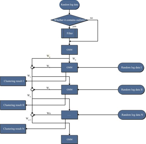When the n-th layer is reached, the initial weights obtained are as follow: (13) ${\hat{z}}_{ki}^{(n-1)n}=\frac{{\hat{z}}_{ki}^{(n-2)(n-1)}+{\hat{z}}_{ki}^n}{2}$(13) In this way, the initialization of each layer will be affected by the previous layer and the filter layer and the filter layers in the block will not have much difference due to random traps. The robustness and generalization ability of the model are greatly enhanced because each GMM integrates the feature distribution of the random well input of the previous layer. The multi-layer GMM model method can be summarized as the following steps:

Step 1: Input the random well data I in the block into the filter;

Step 2: Feed the data output by the filter into the GMM model, and the weight ${\hat{z}}_{ki}^0$ of the last iteration is obtained as the initial weight of the next layer;

Step 3: Let the random well data II be the input of the second layer of GMM model and initialize the weight using the weight ${\hat{z}}_{ki}^0$ of the previous layer, and output the clustering result as well as the weight ${\hat{z}}_{ki}^1$ of the last iteration of the second layer;

Step 4: Let the random well data III be the input of the third layer of GMM model and initialize the weight using the average value of the previous layer and the starting layer to the previous layer (not including the previous layer) for averaging operation;

Step 5: Perform the operation of Step 4 on the remaining N-3 wells in the block in turn, until the N-th layer is reached. In this way, the clustering task is completed for the data of N wells in the block.

The system process of the multi-layer GMM model is shown in Figure 1.

1. D. Double-layer GMM model

Figure 1. Multiple GMM flowchart.

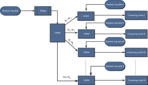
On account of the top-down serial operation mode adopted by the multi-layer GMM and the individual logging data in the block may affect the overall weight, here we give a parallel two-layer GMM model. Due to the use of parallel model, the operation speed will be significantly better than the serial mode, but this will make the random well selection in the first step very important. This is also the main reason why the two-layer GMM model is given, which allows us to perform flexible operations to achieve the desired clustering results.

The main difference between the two-layer GMM model and the multi-layer GMM model is that one GMM unit is added to n in the second layer and the initial weights is used by each GMM unit in this layer that are based on the last iteration of the first layer GMM unit. The generated weight is used as the initial weight. The input of the first layer here is the same as the multi-layer GMM model, which uses the data of random well data after passing the filter as input.

The method of the two-layer GMM model can be summarized as the following steps:

Step 1: Input the random well data I in the block into the filter;

Step 2: Send the data outputted by the filter to the GMM model, and the weight ${\hat{z}}_{ki}^0$ of the first iteration is obtained as the initialization weight of all parallel GMM units in the next layer;

Step 3: Use random well data as the input of each parallel GMM unit, the output is the clustering results. The system process of the GMM model is shown in Figure 2.

Figure 2. Double GMM flowchart.

IV. Analysis of the simulation results

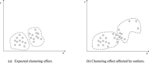
In a two-dimensional space, visualizing data can more intuitively analyze the influence of outliers on GMM. The schematic diagram is as follows:

Due to the influence of outliers, the expected clustering effect shown in Figure 3(a) is prone to changes in Figure 3(b).

Figure 3. Schematic diagram of the influence of outliers.

Although the outliers in the Euclidean space can be removed by calculating the Euclidean distance artificially based on observations and prior knowledge, this pair of high-dimensional spaces (such as Riemann space) makes the outlier Metrics that are difficult to define. It is very difficult to cluster the logging curves with multi-dimensional characteristics because the outliers in the high-dimensional space are difficult to define. Here we select exploratory wells from the block diagram in Figure 4 below to analyze the prior knowledge.

Figure 4. Block well diagram.

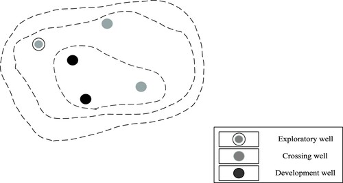
The dotted line in Figure 4 is the contour line. The gray solid with the outer ring is the exploratory well. As the data features of the exploration well are relatively complete, we select it and observe the distribution of the formations and faults in this block according to the logging data to determine whether it is part of the data of the entire interval of the initial well. The result analysis of the best cluster through BIC is shown in Figure 5:

Figure 5. BIC assessment results.

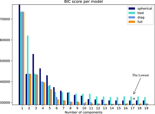
In Figure 5, we have carried out a BIC evaluation of the effects of the 1–20 categories of the model. When using the diagonal covariance matrix (non-diagonal is zero, diagonal is not zero), the Bayes index reaches the lowest and the clustering effect is the best at this time.

The processed initial wells are sent to the multi-layer GMM. And then take the initialization weights generated by the initial wells, the development wells and crossing wells in the block as input. The two-dimensional visualization results of the output difference are shown in Figure 6.

Figure 6. The difference between single and multiple GMM.

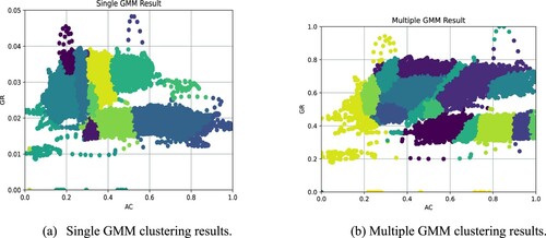
Figure 6(a) shows the results of single-layer GMM clustering with 17 categories. It can be seen that the data is divided extremely unbalanced due to a large number of outliers, and most of the clusters are divided into outliers. And the image is compressed due to the existence of outliers, here we perform the same compression on the normalized Y axis to visualize the original data distribution of the image. Figure 6(b) shows the results of 17 categories after the multi-layer GMM processing. Since we have processed the data of the initial well re ckoned on the prior, the clustering result shows the distribution of the class Gaussian and the distribution among classes is also relatively concentrated, which provides a good precondition for the next evaluation.

Depending to the previous introduction, since the performance of MRGC is the best in the current logging interpretation clustering, we will only compare MRGC and single-layer GMM with double-layer GMM and multilayer GMM in the follow-up. In logging interpretation, we generally considers that the basis for correct classification is depended upon two points: The first is threshold classification: we perform classification operations when logging data is higher/lower than a certain value. The second classification situation is where the difference is obvious: we carry out classification operations at the peak/valley (local) of the logging data. The data is analyzed and visualized with ‘Geolog’ professional logging interpretation software behind clustering. The analysis results are shown in Figures 7 and 8.

Figure 7. The clustering results correspond to the classification of XI well lithofacies.

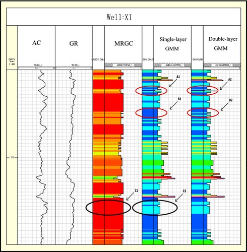
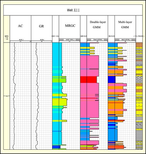
Figure 8. The clustering results correspond to the classification of XII well lithofacies.

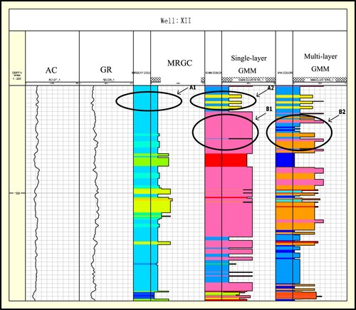
Figure 7 shows the clustering results. The different colors in the rectangle indicate different categories. The length of the rectangle in the figure is just for a clearer visualization and it does not affect the analysis. Firstly, depending on the comparison of C1 and C2, MRGC has divided the high and low values of AC into one category in C1, and no more categories have been found where there is a significant decline in both AC and GR. The cause of this phenomenon is that MRGC uses the KNN kernel, which makes it less sensitive to data fluctuations. Compared with traditional MRGC, GMM has discovered more detailed categories. This means GMM is more sensitive at the peaks and valleys of the curve and it can reflect the trend of stratigraphic changes in time. Secondly, in the comparison between single-layer and double-layer, we have used the better initialization exploratory wells in the block wells for the two-layer GMM model. It can be found a smaller category has been found in the double GMM at the fluctuation of AC and GR relative to the single layer in the comparison of the results of A1, A2 and B1, B2. Finally, this also shows that the given initialization behavior used in the double-layer GMM can better identify the finer classes in the logging curve fluctuation benefit from the overall distribution of the block. Double layer GMM absorbs global prior knowledge to make clustering more sufficient.

Figure 8 shows the clustering results. Due to the use of remote wells near the edge of the block as initialization, this will lead to large initialization error. Therefore, we have adopted the multi-layer GMM model. It can be seen from the fluctuations of AC and GR corresponding to A1, A2 that the performance of single-layer GMM in this segment has been still stronger than MRGC but there will be some fluctuations that cannot be fed back in time as depth increases. Because the multi-layer GMM adopts a connection form similar to the Markov chain, each well can obtain the information of its previous well and store these information. It can be seen from B1 and B2 that even if the isolated remote wells in the block have been selected, the multi-layer GMM can still classify the logging curves more accurately in consideration of the observation data. Multilayer robustness is stronger than double layer.

Figure 9 shows the comparison between the GMM classification results of Well XII and the actual lithology classification. The rightmost is a schematic diagram of lithology at different depths. We have selected core samples with a depth of 1250-1570 m from Well XII. This figure shows the multi-layer GMM method. The classification result is basically consistent with the actual situation, and some depths have errors. The comparison results show that the effect of the multi-layer GMM in this paper is more accurate than the two-layer GMM and MRGC methods.

Figure 9. XII lithology multi-layer GMM classification results and actual comparison.

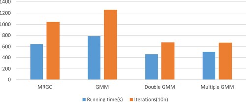
Take the well-positioned XI and the marginal well XIII as the initialization conditions to test their operating efficiency respectively as shown in Figures 10 and 11. It can be seen from the table that the double-layer GMM has the highest efficiency (a shorter time to achieve the expected effect) when the position of the exploratory well is better (XI well), but the efficiency of the multilayer GMM is the highest when the initialization is not good (XIII well).This is because the multi-layer (assuming n-layer) structure has performed n-2 more initialization operations compared to the double-layer structure. Although some time is lost, the multi-layer one achieves higher accuracy than double-layer. After experimentation, we find that both effects are better than other methods.

Figure 10. Operation efficiency of XI as an initialization well.

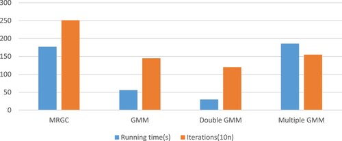
Figure 11. Operation efficiency of XIII as an initialization well.

V. Conclusion

In this paper, a multi-layer GMM and two-layer GMM algorithm are proposed and applied to the cluster interpretation analysis of block wells and strata. The proposed algorithm can more sensitively capture the fluctuation of the logging curve. The multi-layer form adopts the Markov chain mode, which makes the initializing of outliers have less impact on the clustering results and the robustness is greatly enhanced. The advantage of the double layer is that it has a faster effect after the initial layer is given a non-interference initial value, but there is still the problem of being affected by outliers. Subsequently, through subjective visual observation and objective data analysis, the performance of the algorithm is compared with the traditional logging clustering method MRGC and single-layer GMM. The conclusion is that the multi-layer GMM algorithm can reduce the influence of outliers on the clustering results in a certain block and restore the original information of the formation. In future work, we aim to study the parameter selection issues of the multi-layer GMM method, such as how to select accuracy parameters to obtain more accurate clustering results and deal with the noise in the observed logging data (Li et al. (2020); Han et al. (2020); Li et al. (2017); Gao et al. (2020)).

Disclosure statement

No potential conflict of interest was reported by the author(s).

Additional information

Funding

This work was supported in part by Natural Science Foundation of Heilongjiang province F2018004.

REFERENCES

- An, P., & Cao, D. P. (2018). Research and application of logging lithology recognition method based on deep learning. Progress in Geophysics, 33(3), 1029–1034. https://doi.org/https://doi.org/10.6038/pg2018BB0319
- Bergamaschi, S., & Pereira, E. (2001). Characterization of 3rd order depositional sequences for the Siluro-Devonian in the Apucarana Sub-basin, Paraná Basin. Brazil. Ciência Técnica do Petróleo, (20), 63–72.
- Carelli, T., & Borghi, L. (2011). Characterization of sedimentary microfacies in shales of the Ponta Grossa formation (Devonian) on the eastern edge of the Paraná basin. Anuário do Instituto de Geociências - UFRJ, 34(2), 84–104. https://doi.org/https://doi.org/10.11137/2011_2_84-104
- Dypvik, H., & Eriksenf, D. (1983). Natural radioactivity of clastic sediments and the contributions of U, thand K. Journal of Petroleum Geology, 5(4), 409–416. https://doi.org/https://doi.org/10.1111/j.1747-5457.1983.tb00592.x
- Ferreira, F. J. F., Candido, A. G., & Rostirolla, S. P. (2010). Gamma-spectrometric correlation of outcrops and wells: A case study in the Ponta Grossa formation (Paraná Basin, Brazil). Revista Brasileira de Geofisica, 28(3), 371–396. https://doi.org/https://doi.org/10.1590/S0102-261X2010000300005
- Gao, H., Ma, L., Dong, H., Lu, J., & Li, G. (2020). An improved two-dimensional variational mode decomposition algorithm and its application in oil pipeline image. Systems Science and Control Engineering: An Open Access Journal, 8(1), 297–307. https://doi.org/https://doi.org/10.1080/21642583.2020.1756523
- Grahn, Y., Mauller, P. M., Bergamaschi, S., & Bosetti, E. P. (2013). Palynology and sequence stratigraphy of three Devonian rock units in the Apucarana Sub-basin (Paraná Basin, south Brazil): additional data and correlation. Review of Palaeobotany and Palynology, 198, 27–44. https://doi.org/https://doi.org/10.1016/j.revpalbo.2011.10.006
- Han, F., He, Q., Gao, H., Song, J., & Li, J. (2020). Decouple design of leader-following consensus control for nonlinear multi-agent systems. Systems Science and Control Engineering: An Open Access Journal, 8(1), 288–296. https://doi.org/https://doi.org/10.1080/21642583.2020.1748138
- Hao, J. F., Zhou, C. C., & Li, X. (2012). Summary of shale gas evaluation applying geophysical loggings. Progress in Geophysics, 27(4), 1624–1632. doi:https://doi.org/10.6038/j.issn.1004-2093.2012.04.040
- Hu, H., Zeng, H. Y., & Liang, H. B. (2015). Neural network lithology recognition method based on principal component analysis and learning vectorization. Logging Technology, 39(5), 586–590. doi:https://doi.org/10.16489/j.issn.1004-1338.2015.05.09
- Huang, Y. L., Sun, D. Y., & Wang, P. J. (2011). Characteristics of well-logging response to lava flow units of the lower cretaceous basalts in songliao basin. Chinese Journal of Geophysics, 54(2), 169–180. https://doi.org/https://doi.org/10.1002/cjg2.1598
- Johnson, S. (1967). Hierarchical clustering schemes. Psychometrika, 32(3), 241–254. https://doi.org/https://doi.org/10.1007/BF02289588
- Kohonen, T. (1990). The self-organizing map. Proceedings of the IEEE, 78(9), 1464–1480. https://doi.org/https://doi.org/10.1109/5.58325
- Li, J., Dong, H., Han, F., Hou, N., & Li, X. (2017 Jul). Filter design, fault estimation and reliable control for networked time-varying systems: A survey. Systems Science and Control Engineering, 5(1), 331–341. https://doi.org/https://doi.org/10.1080/21642583.2017.1355760
- Li, X., Han, F., Hou, N., Dong, H., & Liu, H. (2020). Set-membership filtering for piecewise linear systems with censored measurements under round-robin protocol. International Journal of Systems Science, 51(9), 1578–1588. https://doi.org/https://doi.org/10.1080/00207721.2020.1768453
- Liu, G. D. (2005). Main problems and countermeasures existed in explorating oil and gas resources in China. Progress in Geophysics, 20(1), 1004–2903. doi:https://doi.org/10.3969/j.issn.1004-2903.2005.01.001
- Mou, D., Wang, Z. W., & Huang, Y. L. (2015). Lithology identification of volcanic rocks based on SVM logging data: Taking the eastern depression of liaohe basin as an example. Journal of Geophysics, 58(5), 1785–1793. doi: CNKI:SUN:DQWX.0.2015-05-028
- Rahsepar, A., Kadkhodaie, A., & Bidhendi, M. (2016). Determination of reservoir electrofacies using clustering methods (MRGC, AHC, SOM, DYNCLUST) throughout ARAB part in SALMAN oil field 2S-05 well. Petroleum Research, 26(87-2), 107–117. https://doi.org/https://doi.org/10.22078/pr.2016.634
- Reynolds, D. (2009). Gaussian mixture models. Encyclopedia of Biometric Recognition, 659–663. https://doi.org/https://doi.org/10.1007/978-0-387-73003-5_196
- Selim, S., & Ismail, M. (1984). K-means-type algorithms: A generalized convergence theorem and characterization of local optimality. IEEE Transactions on Pattern Analysis and Machine Intelligence, PAMI-6(1), 81–87. https://doi.org/https://doi.org/10.1109/TPAMI.1984.4767478
- Shen, B. K., Zhao, H. B., & Cui, W. F. (2012). Sandy conglomerate reservoir logging evaluation study. Progress in Geophysics, 27(3), 1051–1058. doi:https://doi.org/10.6038/j.issn.1004-2903.2012.03.027
- Shi, X. L., Lv, H. Z., & Cui, Y. J. (2018). Log facies division and permeability evaluation based on graph theory multi-resolution clustering method: A case of guantao formation in W well block of Bohai P oilfield. China Offshore Oil and Gas, 30(1), 81–88. doi:https://doi.org/10.11935/j.issn.1673-1506.2018.01.010
- Tan, M. J., & Zhang, S. Y. (2010). Research progress of shale gas reservoir geophysical logging. Progress in Geophysics, 25(6), 2024–2030. doi:https://doi.org/10.3969/j.issn.1004-2903.2010.06.018
- Tan, M. J., & Zhao, W. J. (2006). Description of carbonate reservoirs with NMR log analysis method. Progress in Geophysics, 21(2), 489–493. doi:https://doi.org/10.1016/S1001-8042(06)60011-0
- Tian, Y., Xu, H., & Zhang, X. Y. (2016). Multi-resolution graph-based clustering analysis for lithofacies identification from well log data: Case study of intraplatform bank gas fields, Amu Darya basin. Applied Geophysics, 13(4), 598–607. https://doi.org/https://doi.org/10.1007/s11770-016-0588-3
- Wang, G. W., & Guo, R. K. (2000). Well logging Geology. Petroleum Industry Press, pp. 1-9, 2000.
- Wu, Y. Y., Zhang, W. M., & Tian, C. B. (2013). Application of image logging in identifying lithologies and sedimental facies in reef- shoal carbonate reservoir-take rumaila oil field in Iraq for example. Progress in Geophysics, 28(3), 1497–1506. doi:https://doi.org/10.6038/pg20130345
- Ye, S., & Rabiller, P. (2000). A new tool for electro-facies analysis: multi-resolution graph-based clustering. SPWLA 41st Annual Logging Symposium. Dallas, Texas, pp. 1–14, 2000.
- Ye, S. J., & Rabiller, P. (2005). Automated electrofacies ordering. Petrophysics, 46(6), 409–423. https://onepetro.org/petrophysics/articleabstract/171115/Automated-Electrofacies-Ordering
- Zhang, J. Y. (2012). Well logging evaluation method of shale oil reservoirs and its applications. Progress in Geophysics, 27(3), 1154–1162. doi:https://doi.org/10.6038/j.issn.1004-2903.2012.03.040