Full article: Consumer satisfaction-oriented residential appliance scheduling algorithms

Formulae display: $MathJax Logo$ ?Mathematical formulae have been encoded as MathML and are displayed in this HTML version using MathJax in order to improve their display. Uncheck the box to turn MathJax off. This feature requires Javascript. Click on a formula to zoom.

Abstract

Through effective demand side management, residential energy consumers can enjoy both lower electricity bills and satisfactory electricity-consuming experiences. Lots of residential appliance scheduling algorithms have been proposed, and consumer satisfaction has attracted more and more attention. In this paper, the consumer satisfaction index is defined, and AHP (Analytic Hierarchy Process) is applied to describe the consumer sensitivity to the usage time of each appliance. The time and appliance models are constructed, by use of which the minimum electricity bill model is set up. Based on these models, the consumer satisfaction-oriented residential appliance scheduling algorithm is developed. A case study shows that the new algorithm can help consumers cut down the electricity bill and use the appliances at their favourite time slots. Compared with the consumer's original energy usage scheme, the optimized scheme reduces the electricity bill by 33.56%. At the same time, the Peak-to-Average Ratio can be lowered by 5.26%.

Keywords:

1. Introduction

A smart grid is a digital technology-based electricity network for supplying electricity to consumers via bi-directional digital communication. It can improve the power grid efficiency, reduce energy consumption and cost (Celik & Meral, Citation2019; Fang et al., Citation2012). Since the residential sector in the smart grid contributes to high load, it is necessary to schedule residential appliances effectively to reduce the demand-supply gap (Safdarian et al., Citation2014). Scheduling of residential appliances belongs to demand side management (DSM), and it is an essential part of the smart grid. DSM aims to ensure the efficient and reasonable use of electricity, and at the same time to improve the energy usage habits of consumers (Jin & Mechenhoul, Citation2010). Since it can increase energy efficiency and decrease electricity bills, high-quality DSM is one of the most important parts of power resource management (Hassan et al., Citation2013).

Many research results about DSM have been achieved. Michael et al. built a power consumption model for appliances, such as air conditioners, fridges, and batteries. A mixed-integer linear optimization model was developed to reduce the algorithm complexity (Michael et al., Citation2019). To cultivate good consumer electricity usage behaviours, a modern pricing scheme was proposed (Steriotis et al., Citation2018). A two-stage hierarchical energy management system is designed for smart homes by considering both day-ahead and actual operation stages scheduling (Luo et al., Citation2019). Grey Wolf Optimization based appliance scheduling scheme is presented to reduce electricity cost and PAR (Peak-to-Average Ratio) (Makhadmeh et al., Citation2018). A real-time and price-based home energy management model was propose by Mojtaba et al. This model helps conservative householders save energy and improve energy efficiency through managing electrical appliances (Mojtaba et al., Citation2020). Machine learning algorithms are introduced to DSM in recent years. The reinforcement learning method is applied to find the optimal energy consumption of smart homes with a rooftop solar photovoltaic system, an energy storage system, and smart appliances (Lee & Choi, Citation2019). Consumers' load profiles are put into the input pool for household load forecasting, and deep learning is applied to handle the uncertainty of load profiles (Shi et al., Citation2018). To forecast the load profiles of residential energy management, a novel pooling-based deep neural network was proposed by Jeyaraj et al. This network avoids over-fitting in training and testing by increasing the variety and size of automatic metering infrastructure data (Jeyaraj & Nadar, Citation2021). By introducing an additional inter-supplier cooperation mechanism among consumers, Hupez et al. presented a cooperative demand side management scenario in a low-voltage network considering the context of liberalized electricity markets. They confirmed that the mechanism proposed was able to obtain the minimum cost of all consumers (Hupez et al., Citation2018). A hybrid algorithm combining genetic algorithm and support vector machine was proposed for non-intrusive load monitoring, and the overall accuracy can reach 91.8% (Chui et al., Citation2018).

Consumers become concerning more and more about their life quality, so researchers pay more and more attention to the satisfaction level of consumer electricity usage. Normally, the consumer satisfaction is evaluated in terms of waiting time (Shewale et al., Citation2020). The smaller the waiting time, the closer the starting usage time to what the consumer desires. A hybrid algorithm that integrates the genetic algorithm with the teacher learning-based optimization algorithm was proposed. It describes the relationship among power consumption, cost, and user discomfort region. Consumer discomfort consists of two parts. One is the operation time slot change for time-flexible appliances, and the other is the compression of consumers' demand for power-flexible appliances (Manzoor et al., Citation2017). Economical and user comfortable factors are combined in a multi-objective model proposed by Qu et al., and their simulation shows that the proposed model is effective (Qu et al., Citation2018). An optimization algorithm was proposed to minimize daily energy costs while considering user comfort level and renewable energy consumption rate (Shi et al., Citation2019). Two levels of user satisfaction are defined, i.e. time-based satisfaction and device-based satisfaction (Elavarasan et al., Citation2021). Time-based satisfaction refers to the satisfaction difference when using the same appliance during different time slots. In a given time slot, the use of different appliances brings different satisfaction levels to the consumer. This is the so called device-based satisfaction. The concepts of time-based preference and device-based preference are proposed by Ayub et al., which have the same meaning as those of time-based satisfaction and device-based satisfaction (Ayub et al., Citation2020).

The focus of our proposed residential appliance scheduling algorithms is to decrease the electricity bill while maintaining the comfort degree of consumers on using the appliances. In the literature, the consumer satisfaction level of an appliance is evaluated by the time difference between its actual starting time and the consumer's desired starting time. The satisfaction index in our algorithm is defined similarly, with a few modifications to make its meaning more intuitive. Using the new definition, the larger the satisfaction index, the more comfortable the consumer feels when using the appliances. Normally, a consumer has different sensitivities to the usage time of different appliances. To the best of our knowledge, no current work considers this issue when scheduling appliances. The main contribution of this paper is the introduction of the appliance sensitivity weight to calculate the consumer satisfaction index. The weight of each appliance reflects its importance to the consumer. Our new energy scheduling algorithms help consumers pay less for electricity and use the appliances at their favourite time slots. Additionally, the PAR can also be lowered.

The rest of this paper is organized as follows. Models for our scheduling algorithms are described in Section 2. Section 3 presents the energy scheduling algorithms. Section 4 shows a case study to validate the proposed algorithms. Section 5 gives the conclusion and future work.

2. Models for energy scheduling

Assume that in a smart grid, every family is equipped with a smart metre, and all data from smart metres are shared by power consumers and the corresponding electricity companies. Every appliance can be controlled according to the energy scheduling algorithms. To develop the consumer satisfaction-oriented residential energy scheduling algorithm, the time model and the appliance models should be built first. For the readers' convenience, the parameters in these models are listed in Table .

Table 1. Parameter list.

Display Table

2.1. Time model

A time slot is the time unit used to schedule the working periods for appliances. In most literature, one hour is divided into several time slots for more accurate scheduling. Let the time interval of each time slot be $Δ t$ and $h = 1 / Δ t$ . Then there are h time slots in an hour. Define $h_{max}$ as the total number of time slots in one day, then $h_{max} = 24 \times h$ , and the set of time slots $H = [1, 2, 3, \dots, h_{max}]$ .

2.2. Appliance model

Let AppC be the set of consumer's appliances, e.g. AppC includes a washing machine, an electric kettle, two electric heaters, and an electric vehicle, etc. There are two classifications of appliances, i.e. interruptible and non-interruptible. Non-interruptible appliances cannot be interrupted during their functioning, such as a washing machine. Comparatively, interruptible appliances are those whose tasks can be paused for some time and resumed later, such as an electric heater. $e_{b}^{a}$ is the energy that appliance a consumed during time slot b, and $e_{b}^{a} \geq 0$ , $a \in A p p C$ , $b \in H$ . $E_{a} = {e_{a}^{1}, e_{a}^{2}, \dots, e_{a}^{h_{max}}}$ is the energy used by appliance a during one day. The rated power and standby power of appliance a are $p_{a}^{max}$ and $p_{a}^{min}$ , respectively.

2.2.1. Interruptible appliance model

A sign representing the status of an appliance is introduced in Equation (Equation1(1) $\begin{aligned} f l a g x_{a}^{b} = {\begin{cases} 0 & Appliance a is idle during time slot b \\ 1 & Appliance a is working during time slot b \end{cases} \end{aligned}$ (1) ). (1) $\begin{aligned} f l a g x_{a}^{b} = {\begin{cases} 0 & Appliance a is idle during time slot b \\ 1 & Appliance a is working during time slot b \end{cases} \end{aligned}$ (1) The relationship between $e_{a}^{b}$ and $f l a g x_{a}^{b}$ is shown in Equation (Equation2(2) $e_{a}^{b} = f l a g x_{a}^{b} \times p_{a}^{max} / h + (1 - f l a g x_{a}^{b}) \times p_{a}^{min} / h$ (2) ). (2) $e_{a}^{b} = f l a g x_{a}^{b} \times p_{a}^{max} / h + (1 - f l a g x_{a}^{b}) \times p_{a}^{min} / h$ (2) Assume the maximum energy consumption of each family in one hour is $E_{max}$ , and to avoid circuit overload, for $\forall b \in H$ , it has, (3) $\sum_{a \in A p p C} e_{a}^{b} \leq E_{max} / h$ (3)

2.2.2. Non-interruptible appliance model

Let a be a non-interruptible appliance and its acceptable working period is [ $S_{a}, F_{a}$ ]. $δ_{a}$ is the number of consecutive working time slots of a, $S_{a}$ is the earliest time slot to turn on a, and $F_{a}$ is the latest time slot to turn off a. The variable $f l a g y_{a}^{b}$ shows the time slot to turn on the non-interruptible appliance a, and its definition is shown in Equation (Equation4(4) $\begin{aligned} f l a g y_{a}^{b} = {\begin{cases} 0 & Appliance a is not turned on in time slot b \\ 1 & Appliance a is turned on in time slot b \\ and it continous to work for δ_{a} timeslots \end{cases} \end{aligned}$ (4) ). (4) $\begin{aligned} f l a g y_{a}^{b} = {\begin{cases} 0 & Appliance a is not turned on in time slot b \\ 1 & Appliance a is turned on in time slot b \\ and it continous to work for δ_{a} timeslots \end{cases} \end{aligned}$ (4) (5) $\begin{aligned} \sum_{b = S_{a}}^{F_{a} - δ_{a}} f l a g y_{a}^{b} = 1 a \in A_{u}, b \in [S_{a}, F_{a} - δ_{a}] \end{aligned}$ (5) (6) $\begin{aligned} f l a g y_{a}^{b} = 0 a \in A_{u}, b \notin [S_{a}, F_{a} - δ_{a}] \end{aligned}$ (6) It is clear from Equation (Equation5(5) $\begin{aligned} \sum_{b = S_{a}}^{F_{a} - δ_{a}} f l a g y_{a}^{b} = 1 a \in A_{u}, b \in [S_{a}, F_{a} - δ_{a}] \end{aligned}$ (5) ) that appliance a can be switched on in one of the time slots from $S_{a}$ to $F_{a} - δ_{a}$ . The earliest time slot to turn on a is $S_{a}$ , and to ensure that a can continue to work for $δ_{a}$ time slots before the last turn off time slot $F_{a}$ , the latest time slot to turn on a is the time slot $F_{a} - δ_{a}$ . Equation (Equation6(6) $\begin{aligned} f l a g y_{a}^{b} = 0 a \in A_{u}, b \notin [S_{a}, F_{a} - δ_{a}] \end{aligned}$ (6) ) shows that if the time slot is not within the range $[S_{a}, F_{a} - δ_{a}]$ , appliance a cannot be turned on. Therefore, $f l a g y_{a}^{b} = 0$ .

As the energy consumption is defined using the variable $f l a g x_{a}^{b}$ , the relation between $f l a g y_{a}^{b}$ and $f l a g x_{a}^{b}$ should be found. If a non-interruptible appliance a is turned on in time slot b, and since it continues to work for $δ_{a}$ time slots, it is obvious that, (7) $f l a g x_{a}^{b} = f l a g x_{a}^{b + 1} = f l a g x_{a}^{b + 2} = \dots = f l a g x_{a}^{b + δ_{a} - 1} = 1$ (7) and (8) $e_{a}^{b} = e_{a}^{b + 1} = e_{a}^{b + 2} = \dots = e_{a}^{b + δ_{a} - 1} = p_{a}^{max} / h$ (8) It has, (9) $\begin{aligned} f l a g x_{a}^{b} \geq f l a g y_{a}^{b}, f l a g x_{a}^{b + 1} \geq f l a g y_{a}^{b}, \\ f l a g x_{a}^{b + 2} \geq f l a g y_{a}^{b}, \dots f l a g x_{a}^{b + δ_{a} - 1} \geq f l a g y_{a}^{b} \\ a \in A_{u}, b \in [S_{a}, F_{a} - δ_{a}] \end{aligned}$ (9) Inequality (Equation9(9) $\begin{aligned} f l a g x_{a}^{b} \geq f l a g y_{a}^{b}, f l a g x_{a}^{b + 1} \geq f l a g y_{a}^{b}, \\ f l a g x_{a}^{b + 2} \geq f l a g y_{a}^{b}, \dots f l a g x_{a}^{b + δ_{a} - 1} \geq f l a g y_{a}^{b} \\ a \in A_{u}, b \in [S_{a}, F_{a} - δ_{a}] \end{aligned}$ (9) ) is used in our energy scheduling algorithms to ensure that enough consecutive time slots are provided to a non-interruptive appliance.

2.3. Minimum electricity bill model

Under the variable residential electricity price model, $P R I C E = {p r i c e_{1}, p r i c e_{2}, \dots, p r i c e_{24}}$ is the price set showing the electricity price of each hour in one day, and $p r i c e_{t}$ is the price of the $t th$ hour. The energy consumption $E_{t}$ in the $t th$ hour is represented by Equation (Equation10(10) $E_{t} = \sum_{b = (t - 1) \times h + 1}^{t \times h} \sum_{a \in A p p C} e_{a}^{b}$ (10) ). (10) $E_{t} = \sum_{b = (t - 1) \times h + 1}^{t \times h} \sum_{a \in A p p C} e_{a}^{b}$ (10) where $a \in A p p C$ , $b \in H$ , $t \in {1, 2, 3, \dots, 24}$ . Based on the analysis above, the objective function of the minimum electricity bill model is defined in Equation (Equation11(11) $min \sum_{t = 1}^{24} p r i c e_{t} \times E_{t}$ (11) ). (11) $min \sum_{t = 1}^{24} p r i c e_{t} \times E_{t}$ (11) The constraints are as follows. (12) $\begin{aligned} \sum_{a \in A p p C} e_{a}^{b} \leq E_{max} / h \forall b \in H \end{aligned}$ (12) (13) $\begin{aligned} \sum_{b = S_{a}}^{F_{a} - δ_{a}} f l a g y_{a}^{b} = 1 a \in A_{u}, b \in [S_{a}, F_{a} - δ_{a}] \end{aligned}$ (13) (14) $\begin{aligned} f l a g y_{a}^{b} = 0 a \in A_{u}, b \notin [S_{a}, F_{a} - δ_{a}] \end{aligned}$ (14) (15) $\begin{aligned} \begin{aligned} f l a g x_{a}^{b} \geq f l a g y_{a}^{b} \\ f l a g x_{a}^{b + 1} \geq f l a g y_{a}^{b} \\ f l a g x_{a}^{b + 2} \geq f l a g y_{a}^{b} \\ \dots \\ f l a g x_{a}^{b + δ a - 1} \geq f l a g y_{a}^{b} \\ a \in A_{u}, b \notin [S_{a}, F_{a} - δ_{a}] \end{aligned} \end{aligned}$ (15) (16) $\begin{aligned} \begin{aligned} f l a g x_{a}^{b} \in {0, 1}, a \in A p p C, b \in H \\ f l a g y_{a}^{b} \in {0, 1}, a \in A_{u}, b \in H \end{aligned} \end{aligned}$ (16)

3. Energy scheduling algorithms

Based on the models presented in Section 2, two energy scheduling algorithms are developed.

3.1. Energy scheduling algorithm for the lowest bill

In step 2, under the consideration of the constraints, different combinations of $S_{a}$ and $F_{a}$ for each appliance are tried to calculate the value of $E_{t}$ . It is possible to assign more than one working slot to an interruptible appliance, as long as the total number of working hours satisfies the consumer's requirements. When the most suitable $S_{a}$ and $F_{a}$ for each appliance are found, the minimal electricity cost is obtained.

3.2. Energy scheduling algorithm considering consumers' satisfaction level

In many cases, it is not comfortable enough for the consumers to use their appliances under the optimal scheme aiming at the lowest bill. Electricity cost is not the only issue that consumers concern and they prefer to reduce the cost while enjoying their life. To raise the consumer satisfaction level, we propose a novel energy scheduling algorithm considering consumers' satisfaction. The basic idea is that consumers would like to accept a more comfortable electricity usage scheme, even if it is a little bit more expensive than the lowest bill scheme.

For appliance a, the consumer provides its ideal operation period $[A_{a}, B_{a}]$ and the acceptable operation period $[S_{a}, F_{a}]$ . The closer the scheduled starting time of an appliance is to its ideal starting time, the more comfortable consumers feel when using this device. The consumer satisfaction index $s a t_{a}$ for appliance a is defined in Equation (Equation17(17) $s a t_{a} = 1 - | \frac{r e a l S_{a} - A_{a}}{A_{a} - B_{a}} |$ (17) ). (17) $s a t_{a} = 1 - | \frac{r e a l S_{a} - A_{a}}{A_{a} - B_{a}} |$ (17) Where $r e a l S_{a}$ is the starting time obtained from the energy scheduling algorithm, and $2 A_{a} - B_{a} \leq r e a l S_{a} \leq B_{a}$ . If $r e a l S_{a}$ doesn't lie in this range, $s a t_{a}$ will be a negative number and that is meaningless. It can be seen that $s a t_{a} \in [0, 1]$ .

Generally, consumers have different sensitivity to the usage time of various appliances. For example, they may delay the time for ironing, while they must use the electric cooker at dinner time. A sensitive weight is assigned to each appliance to show its importance to the consumer. AHP (Analytic Hierarchy Process) is chosen to calculate the weight of each appliance under scheduling.

Let $w e i g h t_{a}$ denote the weight of appliance a, the consumer satisfaction level is defined in Equation (Equation18(18) $S a t = \sum_{a \in A p p C} s a t_{a} \times w e i g h t_{a}$ (18) ). (18) $S a t = \sum_{a \in A p p C} s a t_{a} \times w e i g h t_{a}$ (18) A new constraint shown in Equation (Equation19(19) $\sum_{a \in A p p C} S a t \geq t o t a l S a t$ (19) ) should be inserted into the minimum electricity bill model shown in Section 2.3 to reflect the consumer satisfaction level. (19) $\sum_{a \in A p p C} S a t \geq t o t a l S a t$ (19) where totalSat is the acceptable satisfaction level determined by the consumer.

The energy scheduling algorithm with the consideration of consumer satisfaction level is shown inAlgorithm 2.

Similar to Algorithm 1, different combinations of $S_{a}$ and $F_{a}$ for each appliance are examined to calculate the value of $E_{t}$ while keep the consumer satisfaction level meeting the requirement. When the most suitable $S_{a}$ and $F_{a}$ for each appliance are located, the algorithm stops with the output of the optimized scheduling scheme.

4. Case study

Electricity data from a typical family are collected to validate the proposed energy scheduling algorithms. If an appliance's minimum continuous working hours equal its total usage time, then it is non-interruptible. Otherwise, it is interruptible, and discontinuous time slots may be assigned to it.

In this case study, $Δ t = 0.5$ , i.e. one hour has two time slots. So $H_{max} = 48$ and this shows that altogether there are 48 time slots in one day. Assume when appliance a is idle, it doesn't consume energy, i.e. $p_{a}^{min} = 0$ . The maximum energy consumption $E_{max} = 4 kW$ for each consumer. The electricity prices are chosen according to the 2021 Power Grid Tariff of Zhejiang Province, China, as shown in Table .

Table 2. Power grid tariff.

Download CSV Display Table

Table gives the original power usage of the chosen family in one day, and the consumer should pay ¥20.88 for the electricity consumption. Table is the family's power usage plan which describes the basic power usage requirements.

Table 3. Appliances' working slots before scheduling.

Download CSV Display Table

Table 4. Family power usage plan.

Download CSV Display Table

4.1. Simulation for minimum electricity bill scheduling algorithm

According to the appliance information and the consumer's usage plan, Algorithm 1 is executed. The new electricity usage schedule for this family is shown in Table .

Table 5. Appliances' working slots after scheduling.

Download CSV Display Table

Based on the scheduling results, the cost of each appliance is shown in Figure and the family's electricity consumption in 24 hours is shown in Figure .

Figure 1. Electricity bill comparison of each appliance.

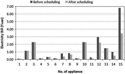
Figure 2. Comparison of hourly electricity consumption.

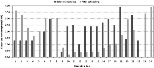
From Figure , it can be seen that the cost of most appliances is cut down. For example, the cost of Appliance 15 is decreased by 49.3%. For this given day, the total cost is ¥20.88 before the scheduling. After scheduling, the cost is only ¥15.55 and the cost reduction is 25.5%. Figure compares the electricity consumption before and after the scheduling in each hour. It is clear that possible peak loads have been shifted to the valley periods, and this contributes to the electricity bill reduction. The working slots of appliances with large power consumption are assigned to the valley periods as many as possible.

4.2. Simulation with considering the consumer satisfaction level

The optimization object of Algorithm 1 is to minimize the electricity cost, and it doesn't consider the consumers' comfort level when using the appliances. Using the scheduling scheme shown in Table , the consumer's satisfaction index is only 0.53. Algorithm 2 is introduced to increase the satisfaction index.

AHP is applied to calculate the sensitivity weight of each appliance listed in Table . After consulting the family, the pairwise comparison matrices were obtained. The consistency ratio CR of each matrix is less than 0.1, so all the matrices pass the consistency check. The weight of each appliance is shown in Table .

Table 6. Sensitivity weight of each appliance.

Download CSV Display Table

In the simulation, the objective consumer satisfaction index is 0.9. The obtained scheme is the so-called Scheme 0.9 thereafter. Using Scheme 0.9, the total cost becomes ¥15.9. Comparing with the ¥15.55 optimal bill, it is only 2.25% higher. Table compares the appliance working slots under these two scheduling schemes. It is clear that under Scheme 0.9 the scheduled working time slots for the appliances are closer to the consumer's desired ones, and the consumer can use these appliances more conveniently.

Table 7. Comparison of the optimal cost scheme and Scheme 0.9.

Download CSV Display Table

Using Algorithm 2, when the value of the satisfaction index is reduced to 0.85, we can also achieve the optimal cost of ¥15.55. Actually, Algorithm 1 can find all the possible scheduling schemes which yield the optimal cost, and then the one with the highest satisfaction index can be provided to the consumers for theirchoice.

Figure shows the satisfaction index of each appliance under Scheme 0.9. It can be seen that except for the vacuum cleaner (No. 7), the consumer can use the appliances comfortably. Figure gives the relationship between the electricity bill and the satisfaction index.

Figure 3. The satisfaction index of each appliance.

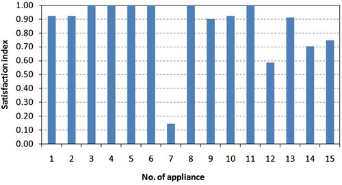
Figure 4. Relationship between the electricity bill and the satisfaction index.

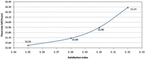
Figure shows that when the consumer satisfaction index is low, it doesn't cost too much to raise the consumer's comfort level, e.g. only 0.9% extra cost is enough to raise the satisfaction index from 0.85 to 0.88. While with the increase of the satisfaction index, the cost for raising the satisfaction index also increases. 2.45% extra cost is needed to raise the satisfaction index from 0.90to 0.92.

4.3. Comparison with other models

In this section, our algorithm is compared with the algorithm proposed by Lu et al. (Citation2014). They proposed two appliances scheduling algorithms. One is to minimize the peak time electricity consumption, and the other is to minimize the total electricity cost. The genetic algorithm is used to find the optimized solutions. As Lu didn't consider the consumer satisfaction level, and our objective is to minimize the electricity bill, we compare Algorithm 1 with the electricity cost optimization algorithm of Lu. The data for the experiments are taken from Lu's paper and it is included in the Appendix. Figure gives the simulation results.

Figure 5. The results of the comparison experiments. (a) Electricity bill and (b) Peak-to-average ratio.

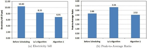
From Figure , it is clear that our algorithm outperforms Lu's algorithm. Compared with the original energy consumption scheme, our algorithm saves 33.56% of the cost, and the saving of Lu's algorithm is 19.90%. For PAR, the lower, the better. The PAR produced by our algorithm is 5.26% lower than that of the original scheme, while Lu's algorithm doesn't show a goodperformance.

5. Conclusion

In this paper, we propose a consumer satisfaction-oriented residential appliance scheduling algorithm to reduce the electricity cost, and at the same time to maintain the consumers' satisfaction level when using the appliances. After obtaining the information of the appliances and the consumer electricity usage requirements, optimized energy scheduling schemes are provided. The results of a case study show that the proposed algorithm can not only lower electricity bill but also allow consumers to use the appliances at their convenience. Compared with the original energy usage scheme of the consumer, our algorithm can reduce the electricity bill and lower the PAR.

In the current work, the optimization is applied to one family. When all families in one community use the scheduling schemes simultaneously, electricity peak valley inversion may occur. To handle this issue, the energy scheduling for a whole community will be considered in our future work.

Disclosure statement

No potential conflict of interest was reported by the author(s).

Data availability statement

All data, models used during the study appear in the submitted article.

Additional information

Funding

This work was supported by National Key R&D Program of China (No. 2018YFB0204003).

References

Ayub, S., Ayob, S. M., Tan, C. W., Ayub, L., & Bukar, A. L. (2020). Optimal residence energy management with time and device-based preferences using an enhanced binary grey wolf optimization algorithm. Sustainable Energy Technologies and Assessments, (41). https://doi.org/https://doi.org/10.1016/j.seta.2020.100798.
Google Scholar
Celik, D., & Meral, M. E. (2019). Current control based power management strategy for distributed power generation system. Control Engineering Practice, 82, 72–85. https://doi.org/https://doi.org/10.1016/j.conengprac.2018.09.025
Web of Science ®Google Scholar
Chui, K. T., Lytras, M. D., & Visvizi, A. (2018). Energy sustainability in smart cities: Artificial intelligence, smart monitoring, and optimization of energy consumption. Energies, 11(11), 2869. https://doi.org/https://doi.org/10.3390/en11112869
Web of Science ®Google Scholar
Elavarasan, R. M., Leoponraj, S., Vishnupriyan, J., Dheeraj, A., & Sundar, G. G. (2021). Multi-criteria decision analysis for user satisfaction-induced demand-side load management for an institutional building. Renewable Energy, 170, 1396–1426. https://doi.org/https://doi.org/10.1016/j.renene.2021.01.134
Web of Science ®Google Scholar
Fang, X., Misra, S., Xue, G., & Yang, D. (2012). Smart grid-The new and improved power grid: A survey. Communications Survey & Tutorials, 14(4), 944–980. https://doi.org/https://doi.org/10.1109/SURV.2011.101911.00087
Web of Science ®Google Scholar
Hassan, E. H., Maaroufi, M., & Quassaid, M. (2013). Demand side management algorithms and modeling in smart grids A customer's behavior based study. In IEEE department of electrical engineering.
Google Scholar
Hupez, M., Greve, Z. D., & Vallee, F. (2018). Cooperative demand-side management scenario for the low-voltage network in liberalised electricity markets. IET Generation, Transmission & Distribution, 12(22), 5990–5999. https://doi.org/https://doi.org/10.1049/gtd2.v12.22
Web of Science ®Google Scholar
Jeyaraj, P. R., & Nadar, E. R. S. (2021). Computer-assisted demand-side energy management in residential smart grid employing novel pooling deep learning algorithm. International Journal of Energy Research, 45(5), 7961–7973. https://doi.org/https://doi.org/10.1002/er.v45.5
Web of Science ®Google Scholar
Jin, T. D., & Mechenhoul, M. (2010). Ordering electricity via internet and its potentials for smart grid systems. IEEE Transactions On Smart Grid, 1(3), 302–310. https://doi.org/https://doi.org/10.1109/TSG.2010.2072995
Web of Science ®Google Scholar
Lee, S., & Choi, D. H. (2019). Reinforcement learning-based energy management of smart home with rooftop solar photovoltaic system, energy storage system, and home appliances. Sensors, 19(18), 3937–3959. https://doi.org/https://doi.org/10.3390/s19183937
Web of Science ®Google Scholar
Lu, Q., Xie, P. J., Leng, Y. J., Hou, J. C., & Sun, B. (2014). Optimization of electricity consumption task scheduling for household smart electricity consumption. Ease China Electric Power, 42(5), 816–821.
Google Scholar
Luo, F., Ranzi, G., Wang, S., & Dong, Z. Y. (2019). Hierarchical energy management system for home microgrids. IEEE Transactions On Smart Grid, 10(5), 5536–5546. https://doi.org/https://doi.org/10.1109/TSG.5165411
Web of Science ®Google Scholar
Makhadmeh, S. N., Khader, A. T., Al-Betar, M. A., & Naim, S. (2018). An optimal power scheduling for smart home appliances with smart battery using grey wolf optimizer. In IEEE international conference on control system, computing and engineering (ICCSCE) (pp. 76–81).
Google Scholar
Manzoor, A., Javaid, N., Ullah, I., Abdul, W., Almogren, A., & Alamri, A. (2017). An intelligent hybrid heuristic scheme for smart metering based demand side management in smart homes. Energies, 10(9), 1–28. https://doi.org/https://doi.org/10.3390/en10-091258
Web of Science ®Google Scholar
Michael, D. S. D., Miguel, F. A., & Sebastien, L. D. (2019). A realistic energy optimization model for smart-home appliances. International Journal of Energy Research, 43(8), 3237–3263. https://doi.org/https://doi.org/10.1002/er.v43.8
Web of Science ®Google Scholar
Mojtaba, M., Mohsen, A., & Salman, K. (2020). Demand response management in smart homes using robust optimization. Electric Power Components and Systems, 48(8), 817–832. https://doi.org/https://doi.org/10.1080/15325008.2020.1821831.
Web of Science ®Google Scholar
Qu, Z. Y., Han, J., & Qu, N. (2018). Multi-objective optimization model of electricity consumption behavior considering combination of household appliance correlation and comfort. Automation of Electric Power System, 42(2), 50–57. https://doi.org/https://doi.org/10.7500/AEPS20170613013.
Google Scholar
Safdarian, A., Fotuhi-Firuzabad, M., & Lehtonen, M. (2014). Benefits of demand response on operation of distribution networks: A case study. IEEE Systems Journal, 10(1), 189–197. https://doi.org/https://doi.org/10.1109/JSYST.2013.2297792
Web of Science ®Google Scholar
Shewale, A., Mokhade, A., Funde, N., & Bokde, N. D. (2020). An overview of demand response in smart grid and optimization techniques for efficient residential appliance scheduling problem. Energies, 13(16), 4266. https://doi.org/https://doi.org/10.3390/en13164266
Web of Science ®Google Scholar
Shi, H., Xu, M., & Li, R. (2018). Deep learning for household load forecasting – a novel pooling deep RNN. IEEE Transactions on Smart Grid, 9(5), 5271–5280. https://doi.org/https://doi.org/10.1109/TSG.516-5411
Web of Science ®Google Scholar
Shi, K., Li, D., Gong, T., Dong, M., Gong, F., & Sun, Y. (2019). Smart community energy cost optimization taking user comfort level and renewable energy consumption rate into consideration. Process, 7(2), 1–17. https://doi.org/https://doi.org/10.3390/pr7020063.
Web of Science ®Google Scholar
Steriotis, K., Tsaousoglou, G., Efthymiopoulos, N., Makris, P., & Varvarigos, E. (2018). Development of real time energy pricing schemes that incentivize behavioral changes. In IEEE international energy conference/IEEE ENERGYCON.
Google Scholar

Appendix

The data used in the case study are shown in Table .

Table A1. Data used in Section 4.3

Download CSV Display Table

Consumer satisfaction-oriented residential appliance scheduling algorithms

Abstract

1. Introduction