A review: data driven-based fault diagnosis and RUL prediction of petroleum machinery and equipment

Abstract

In this paper, an up-to-date overview is provided on the data driven-based fault diagnosis (FD) and remaining useful life (RUL) prediction problems of the petroleum machinery and equipment (PME). First, the FD and RUL prediction of five key components including bearings, gears, motors, pumps and pipelines are discussed by adopting mathematical statistics and shallow learning. Then, four kinds of widely-used DL models, i.e. deep neural networks, deep belief networks, convolution neural networks and recurrent neural networks, are surveyed, and the applications in the field of PME are highlighted. Finally, the possible challenges are proposed and some corresponding research directions in the future are presented.

Keywords:

• Petroleum machinery and equipment
• fault diagnosis
• remaining useful life prediction
• mathematical statistics
• shallow learning
• deep learning

1. Introduction

Serving as one of the most important roles in the petroleum industry, the petroleum machinery and equipment (PME) has received particular research attention such as the pipelines and the pumping units. Note that the construction of the pipelines not only increases the transport volume of the oil but also reduces the cost of the transportation. In addition, as the core equipment for oil exploitation, the pumping unit has been gaining an ever-increasing research attention, especially the smooth operation which is the basic requirement for oil production. Nevertheless, it is worth noting that once these equipments fail, the economic losses and casualties are unpredictable. For example, as for the pipelines, the long-time work will lead to the aging of the anti-corrosion layers, which probably brings corrosion perforation, leakage, rupture and other accidents. With regard to the pumping units, the crank pin fracture always results in frame torsion, gearbox overturning and other serious accidents. Moreover, the frequently occurred failures of the gear and bearing of pumping unit gearbox will severely affect the oil productions and the economic benefits. To solve these problems, the fault diagnosis (FD) and the remaining useful life (RUL) prediction issues of the PME have attracted tremendous research attention, which aim to ensure the safety production (Heng et al., 2009).

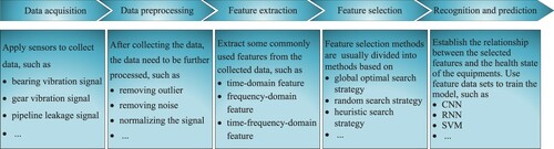
Till now, the researchers have paid much attention to the FD and RUL problems, see Layouni et al. (2017), S. Zhao et al. (2020), Shaik et al. (2020), Zadkarami et al. (2020) and the reference therein. In general, the FD and RUL are roughly divided into five steps as demonstrated in Figure 1: data acquisition, data preprocessing, feature extraction, feature selection as well as recognition and prediction. Taking the bearing of the pumping unit as an example, the five steps are explained as follows. (1) Data acquisition refers to the vibration signal collections of the bearings from the installed acceleration sensors; (2) Data preprocessing aims to remove the outliers and noise by some methods (2021; L. Zou et al., in press-a), and then carries on the signal normalization; (3) The purpose of feature extraction is to extract some commonly used features including obvious features and implicit features from the collected data. To be more specific, the obvious features mainly include the time-domain features, frequency-domain features and time-frequency-domain features, and the implicit features are those learned autonomously by models such as deep learning (DL); (4) Generally speaking, according to different search strategies, the methods of feature selection can be classified into three categories on the basis of global optimal search strategy, random search strategy (e.g. relief algorithm Kira & Rendell, 1992), and heuristic search strategy (e.g. sequence forward selection algorithm Ververidis & Kotropoulos, 2005). The proposed selection methods are employed to select the features that are sensitive to the health states of the bearings from the extracted features so as to further improve the accuracy of the FD; and (5) Finally, by using the feature data sets, the purpose of recognition and prediction is to train the model for establishing the relationship between the selected features and the health states of the equipments. In view of this, for an unmarked vibration signal sample of the bearings, the model can identify the health states of the bearings and predict the RUL of them.

Figure 1. Five steps of FD and RUL prediction.

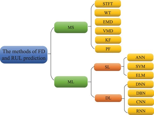
Generally speaking, the methods of FD and RUL prediction can be divided into the mathematical statistics (MS) method and the machine learning (ML) method. Specifically, the MS method mainly includes short-time Fourier transform (STFT) (Nawab et al., 1983), wavelet transform (WT) (Daubechies, 1990), empirical mode decomposition (EMD) (N. E. Huang et al., 1998), variational mode decomposition (VMD) (Dragomiretskiy & Zosso, 2014), Kalman filtering (KF) (Kalman & Bucy, 1961) and particle filtering (PF) (Carpenter et al., 1999). As the core of artificial intelligence, the ML has been widely used in data mining (Nguyen et al., 2019), speech recognition (Padmanabhan & Premkumar, 2015), FD (Lei et al., 2020; R. Liu et al., 2018), RUL prediction (Lei et al., 2018; Y. Wang, Zhao, et al., 2020) and other fields. Furthermore, the ML-based FD and RUL prediction method can be further divided into shallow learning (SL) method and DL method. The SL mainly contains artificial neural networks (ANN) (Jain et al., 1996), extreme learning machine (ELM) (G. Huang et al., 2006) and support vector machine (SVM) (Cortes & Vapnik, 1995). The DL mainly contains deep neural networks (DNN) (W. Liu et al., 2017), convolution neural networks (CNN) (Gu et al., 2018), deep belief networks (DBN) (Sarikaya et al., 2014) and recurrent neural networks (RNN) (Mikolov et al., 2011). The classification of the FD and RUL prediction methods is presented in Figure 2.

Figure 2. The methods of FD and RUL prediction.

In order to extract and select the features of the running states of the PME, the MS method has been employed which, however, can only provide good diagnosis and prediction results for small-scale data. That is to say, it is difficult to process and analyse massive data automatically through the MS. Among the ML methods, the SL method is not expert in expressing complex functions when the samples and computing units are limited. In the recent years, the DL model has attracted much attention (Hinton et al., 2006), which is capable of extracting features from the source signals adaptively and avoiding the impacts from the artificial feature extraction. Moreover, owing to the emphasis on the depth of the model structure, DL has a good generalization ability and thus the low nonlinear performance of the shallow neural networks can be well solved. In addition, DL is capable of transforming the feature representations of the samples in the original space into the representations in a new feature space through layer-by-layer feature transformation, which makes it easy to classify the faults and predict the RUL. The unique advantages of DL provide a new idea for the research on FD and RUL prediction of the PME (J. Feng et al., 2018; Georg & Matthias, 2018). It is worth mentioning that the combination of other methods and DL has become a research focus, and some pioneering results have been reported. The main contributions of this paper can be highlighted as follows:

1. We have reviewed all searchable articles of DL for fault diagnosis and RUL prediction of PME.

2. Four kinds of widely-used DL models, i.e. DNN, DBN, CNN and RNN, are surveyed, and the applications in the field of PME are highlighted.

3. To the best of our knowledge, this is the first comprehensive DL survey for FD and RUL prediction of PME.

4. We have reviewed the current status of the DL in FD and RUL prediction of PME and also highlighted the future opportunities.

The remaining sections of this paper are organized as follows. Several main methods based on MS and SL with their applications in FD and RUL prediction of the PME are introduced in Section 2. Then a few major methods based on DL with their applications in FD and RUL prediction of the PME are highlighted in Section 3. The possible challenges, research topics in the future and some corresponding research directions are summarized in Section 4.

2. Fault diagnosis and remaining useful life prediction based on mathematical statistics and shallow learning

In this section, a review of FD and RUL prediction methods based on MS and SL is given. First, some components of the oil production and transportation equipments are listed. Then, the FD and RUL prediction methods based on the MS and SL are introduced.

2.1. Important components of PME

In general, the PME is divided into the oil production equipments (e.g. pumping unit, hydraulic oil production devices and drilling rig) and the oil transportation equipments (e.g. pipeline and screw pump).

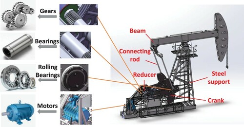
When it comes to the oil production equipments, the pumping unit will be the first one to be considered. As shown in Figure 3, the pumping unit is powered by the motor all the time (C. Zhang et al., 2020). The reducer of the pumping unit is an internal meshing transmission device composed of internal gears and external gears, which is responsible for reducing the speed of the motor. It should be noted that the crank and the connecting rod are connected by rolling bearings, then the beam and the steel support are connected by the bearings in the pumping unit. Furthermore, it can be observed from Figure 3 that the bearings exist in the reducer as well. For other oil production equipments such as hydraulic oil production devices and drilling rigs, the components like pumps are critical to their work.

Figure 3. The structure diagram of the pumping unit.

It is well recognized that pipelines have been the main oil transportation equipments in the past decades. The reasons for adopting pipelines to transport oil are twofold. One is that the transportation volume of them is large and the transportation cost is low. The other one is that the pipelines are buried underground deeply, so they occupy a relatively smaller area and are less affected by the climates and environments. Moreover, as another kind of important component, the screw pump is often chosen to connect with the pipelines due to that it does not form the turbulence and is not sensitive to the viscosity of the medium (Alves et al., 2011).

It is concluded from the previous contents that the components such as bearings, gears, pumps, motors and pipelines are playing extremely important roles in the work of the PME. Once the components work under high load and harsh environment without timely repair and maintenance, the components will be vulnerable to wear and corrosion over a long period of time. As demonstrated in Figure 4, two types of faults frequently occur in bearings, namely, the inner ring wear and the outer ring wear. Additionally, the gears often break down including cracking, wearing and fracturing. Consequently, it is of great significance to implement FD and RUL prediction for the components. Then some typical equipments and their main components with requirement on FD and RUL prediction are shown in Figure 5.

Figure 4. Diagrams of the failure of bearings and gears.

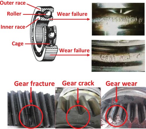
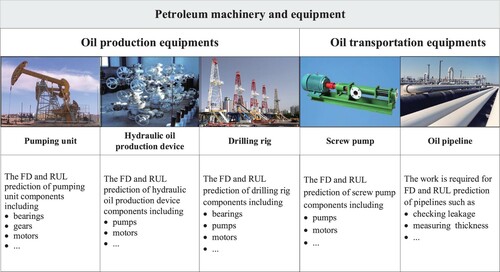
Figure 5. Typical PME and their main components.

2.2. Methods based on mathematical statistics

2.2.1. Short-time Fourier transform

It is claimed that Fourier transform is a commonly used mathematical transform method. As a significant extended signal processing method, the STFT has been proposed by Gabor in 1946, with the purpose of analysing non-stationary signals (Gabor, 1946). During the past years, with great efforts, some researchers have made some achievements in applying STFT to the FD of bearings (H. Li et al., 2019; Y. Zhang et al., 2020), gears (Bian et al., 2019) and pumps (W. Zhao et al., 2016).

Particularly, the combination of other methods and STFT has attracted plenty of research attention. Y. Zhang et al. (2020) have adopted STFT and CNN to diagnose faults of bearings. In the proposed method, the STFT has been employed to obtain the input images of the bearing inner and outer race fault signals. After that, the extracted features have been fed into the CNN to diagnose faults sequentially. Similarly, in H. Li et al. (2019), the STFT has also been combined with the CNN, in which the STFT has been used to obtain the time-frequency spectrum samples of the vibration signals of rolling bearings. Jointly with CNN, the end-to-end fault pattern recognition has been realized. Moreover, the STFT has been applied to the transformation of signal dimensions as well. For instance, in Bian et al. (2019), the one-dimensional vibration signals have been transformed into a two-dimensional spectrogram by STFT, and then the obtained image has been input into the trained CNN model, which has achieved the FD of the gearboxes.

2.2.2. Wavelet transform

The WT has a time-frequency window that changes with frequency. The main idea of WT is to decompose a signal into a series of wavelets. It is worth mentioning that WT can fully highlight the characteristics of the considered problems and overcome the weaknesses that the window size of STFT does not change with frequency and the time resolution and the frequency resolution cannot achieve the best simultaneously (H. Sun et al., 2014). Inspired by J. Chen et al. (2016), we have reviewed some practical applications during the past few years. In Liang et al. (2019), the WT has been combined with constructed multi-label CNN to diagnose the faults of the gears. To be specific, the two-dimensional time-frequency features have been extracted from the original one-dimensional vibration signals by WT and then input into the multi-label CNN model to further diagnose the faults with examples including fracture and cracking. Moreover, we have found many other variants of WT applied in FD, which include continuous WT (Ahuja et al., 2020; Parey & Singh, 2019), discrete WT (Bajric et al., 2016; R. Chen et al., 2019; Kordestani et al., 2018), wavelet packet transform (Islam & Kim, 2019; Wan & Zhang, 2018; L. Wang, Liu, et al., 2020) and empirical WT (H. Yu et al., 2020; X. Zhang et al., 2019; Z. Zheng et al., 2019).

The continuous WT has been ever employed to decompose the angular domain averaged signals of the gearboxes (Parey & Singh, 2019). The obtained acoustic features such as crack and fracture have been compared with those of healthy gears, and then the optimal scale range has been determined according to the energy-Shannon's entropy ratio of the continuous wavelet coefficients. In R. Chen et al. (2019), discrete WT, another variant of WT, has been used to identify the different health states of the gearboxes by combining with the CNN. In this method, discrete WT is capable of giving a more prominent and comprehensive representation of time-frequency distribution of the concerned signals, which is input into the trained CNN model for further FD. In addition, in order to analyse the inherent defect information consisting of different sizes of cracks on the outer, inner and roller raceway in bearing fault signals, the wavelet packet transform has been applied to quantify the input signals into plenty of low and high-frequency sub-bands signals, which have been fed into an adaptive deep CNN (Islam & Kim, 2019). In H. Yu et al. (2020), the empirical WT has been used to decompose the three-channel signals of hydraulic pump into several AM-FM components, the weights of which have been measured through the defined variance contribution rate. Furthermore, the spatial clustering algorithm has been employed to improve the performance of the empirical WT in the whole space, which has solved the improper spectrum segmentation problem of the empirical WT.

2.2.3. Empirical mode decomposition

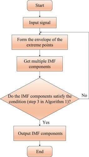
The EMD adaptively decomposes the signals through the time-scale features of the data themselves with no requirement on setting any basic functions, which is essentially different from the wavelet decomposition method based on wavelet basis functions. Therefore, the EMD can be applied to the decomposition of any types of signals theoretically. It is widely recognized that the EMD has been exploited in signal processing (Das et al., 2020; L. Liu et al., 2020; J. Zheng & Pan, 2020), data feature analysis (Aziz et al., 2019; Q. Li, Zheng, et al., 2020; Mondal et al., 2018) and FD (Abdelkader et al., 2016, 2018; Alabied et al., 2018; Cheng et al., 2019; C. Guo et al., 2016; Park et al., 2018; Xu et al., 2020; Xue et al., 2015). In Xu et al. (2020), according to the frequency features of the signals processed by the combination of EMD and Hilbert transform, both the flexural wave and the longitudinal wave have been selected for the localization. Then the leakage sources in the pipelines have been located through the peak magnitude corresponding to the arrival time of the guided waves. During the past decades, breakthroughs on improving EMD have been achieved with examples including fast EMD (Y. Wang, Zhu, et al., 2020), median EMD (Karatoprak & Seker, 2019) and ensemble EMD (Abdelkader et al., 2018; Cheng et al., 2019; Park et al., 2018; L. Wang & Shao, 2020; Xue et al., 2015; Yeh et al., 2010). To be specific, the EMD algorithm is illustrated in Algorithm 1 (Lei et al., 2013) and the decomposition process is shown in Figure 6.

Figure 6. The decomposition of the EMD algorithm.

For improving the computation speed and inhibiting the phenomenon of modal over-decomposition of the EMD, the fast EMD has been proposed in Y. H. Wang et al. (2014). In Y. Wang, Zhu, et al. (2020), the fast EMD has been employed to automatically separate the original signals of the hydraulic pump in the FD of hydraulic pump, then the useful components of signals have been obtained by measuring the relative entropy. As another variant of EMD, the median EMD has added a process in which the decomposed IMFs have been filtered by a variable window sized median filter and summed again to recompose the signals. In Karatoprak and Seker (2019), the fault features of the motor have been extracted by the median EMD, thus the mode-mixing has been reduced and the fundamental frequency of each IMF has been separated. In Park et al. (2018), the ensemble EMD has been employed to extract fault features from transmission error signals of faulty gears under the noisy environment, then the k-nearest neighbour algorithm has been adopted to classify faults. Furthermore, it should be noted that ensemble EMD has evolved into some variants containing adaptive fast ensemble EMD (Xue et al., 2015) and complementary ensemble EMD (Cheng et al., 2019; Yeh et al., 2010) in the past few years. With respect to complementary ensemble EMD, it has been designed to reduce the computation time of the ensemble EMD, in which the pairs of complementary ensemble IMFs with positive and negative white noises have been introduced to eliminate the residue noises in the IMFs (Yeh et al., 2010). On the basis of the complementary ensemble EMD, the noises in pairs of positive and negative have been added to the residue signals for the sake of reducing the reconstruction errors and mitigating the effects of mode mixing. The above mentioned method has been adopted to analyse the non-stationary vibration signals of rolling bearings in the FD for bearings (Cheng et al., 2019).

2.2.4. Variational mode decomposition

The EMD is often accompanied by the phenomena of end effects and aliasing of modal components. With the purpose of solving these problems, the VMD has been proposed to deal with the non-stationary sequence signals, which is capable of determining the numbers of the mode decomposition of the given sequence according to the practice. Furthermore, in order to separate the IMFs effectively and divide the signals in frequency domain, the VMD adaptively matches the optimal central frequency and the finite bandwidth of each mode in the process of searching and seeking the solution. For clarity, the complete algorithm of the VMD is given in Algorithm 2 (Dragomiretskiy & Zosso, 2014). It is worth noting that the VMD has been adopted in the area of FD for a variety of equipments with examples including motors, pipelines and gears in the past decade (Y. Chen et al., 2019; Choi et al., 2018; Diao et al., 2020; Z. Guo et al., 2019; Ju et al., 2019; Y. Li, Li, et al., 2018; Z. Li et al., 2018; Y. Liu et al., 2016; Miao et al., 2019; Yan, Liu, Zhang, et al., 2020; X. Zhang et al., 2018; S. Zhao et al., 2020; D. Zou & Ge, 2019).

In D. Zou and Ge (2019), the singular value decomposition has been adopted to calculate the effective numbers of the band-limited IMF of VMD. In order to observe the frequencies of the fault features of the motors, the filtered stator current is divided into finite band-limited IMFs through VMD decomposing, and then the Hilbert transform has been performed on each band-limited IMF. The proposed method is convenient to observe the fault characteristic frequencies from the processing results. Also processing signals with original VMD, in Y. Chen et al. (2019), the VMD has been employed to process the check valve vibration signals in different states. Next, the feature vector set formed by the extracted different features of each layer of IMF components has been processed by vector quantization, which are then input into models so as to identify the fault types of the check valves.

It is worth noting that the intelligent optimization algorithms have developed rapidly in recent years, such as particle swarm optimization (PSO) algorithm (W. Liu, Wang, Yuan, et al., 2021; C. Wang, Han, Shen, et al., 2020). The optimization problems of the parameters of VMD through swarm intelligence algorithms have stirred a great deal of attention (Diao et al., 2020; Yan, Liu, Zhang, et al., 2020; S. Zhao et al., 2020), which mainly include particle swarm optimization (PSO) algorithm and grey wolf optimization (GWO) algorithm. In Diao et al. (2020), the PSO has been adopted to self-select the VMD parameter pair for removing the background noise from pipeline leakage signal more accurately. In Yan, Liu, Zhang, et al. (2020), the GWO algorithm has been employed to determine the inside parameters of the VMD for the FD of rotors.

In addition, it is worth pointing that adaptive mechanism has shown prominent place in terms of parameter optimization (Elsayed et al., 2017; Miao et al., 2019; Zamuda, 2017; X. Zhang et al., 2018). A parameter adaptive VMD method based on grasshopper optimization algorithm (GOA) has been shown in X. Zhang et al. (2018) for the sake of analysing the vibration signals of rotating machinery. Taking the weighted kurtosis index constructed by the kurtosis index and correlation coefficient as the optimization objective, the GOA algorithm has been adopted to optimize the VMD parameters for the extractions of the fault features. Similarly, towards the parameter adaptive VMD for FD, Miao et al. (2019) has shown another index to be the optimization objective, namely, ensemble kurtosis. The improved method has performed great improvements on the FD of bearings.

2.2.5. Kalman filtering

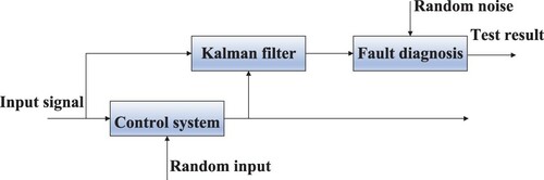
In recent years, the filtering has developed greatly, such as the set-membership filtering (Ding et al., 2020; X. Li et al., 2020; L. Liu et al., 2021; Z. Zhao et al., 2020), the recursive filtering (Hu et al., 2017; B. Shen et al., 2020; L. Wang, Wang, et al., 2020), the distributed filtering (Q. Li, Shen, et al., 2020; Ma et al., 2019) and so on (Ge et al., 2019; B. Shen et al., 2019; Tian et al., 2019; L. Zou et al., in press-b). As for the field of FD and RUL prediction, two main filtering methods, KF and PF, have been given a lot of attention. In 1961, KF, another method has been proposed by R. E. Kalman, which is an algorithm for optimal estimation of system states by using system state evolutions and observation data (Kalman & Bucy, 1961). It should be noted that the KF is capable of improving the weakness that the signals and noises must be stationary in Wiener filtering (Kalman, 1960). During the past few years, the KF has been improved a lot (Ding et al., 2019), and the KF has been widely used in the fields of target tracking (Jondhale & Deshpande, 2019a, 2019b; X. Wang et al., 2020), state estimation (Z. Wang et al., 2017; Zanni et al., 2017; S. Zhao et al., 2017), signal processing (Dai et al., 2017), FD and RUL prediction (Asl et al., 2019; Cui et al., 2019, 2020; Z. Feng et al., 2019; Kandukuri et al., 2019; Y. Li et al., 2019; Lim & Mba, 2015; Moulahi & Hmida, 2020; Naseri et al., 2020; Singleton et al., 2015; Son et al., 2016), etc. The process of the FD based on the KF is described in Figure 7. In recent years, many variants of the KF algorithm have emerged, and the switching KF (Lim & Mba, 2015), unscented KF (Asl et al., 2019; Cui et al., 2019), extended KF (Moulahi & Hmida, 2020; Singleton et al., 2015) and vold-KF (Z. Feng et al., 2019; Kandukuri et al., 2019; Y. Li et al., 2019) have attracted massive attention of scholars.

Figure 7. The process of FD based on KF.

Cui et al. (2020) have constructed two KF models based on linear function and quadratic function, which have been applied to analysing slow degradation stages and accelerated degradation stage of the evolution of the monitoring data of the bearings, respectively. In addition, the relative error of the sliding window has been constructed to adaptively judge the bearing degradation stages. Also aiming at the bearing degradation, Lim and Mba (2015) has introduced the switching KF. In Asl et al. (2019), the switching KF based on state-space method has been adopted to infer different bearing degradation processes and applied to the life prediction of bearings successfully. An adaptive square-root unscented KF has been proposed for leakage FD in a hydraulic system, which can adaptively estimate the means and covariances of the process noises, the measurement noises as well as the system states. Motivated by Lim and Mba (2015) and Asl et al. (2019), a new switching unscented KF has been utilized to predict the RUL of the bearings. The measurement error parameters of the filter have been selected as the standard deviation of condition monitoring data in the degradation state, which can effectively filter out the fluctuation characteristics of the data (Cui et al., 2019). Owing to the ability to deal with the nonlinear system, the extended KF has been adopted to predict the RUL of bearings under different operating conditions, in which the best approximating analytical function has been employed to learn the parameters of the extended KF. Furthermore, the extended KF has been widely applied in the RUL prediction of pipelines, see Moulahi and Hmida (2020). As another variant of KF, the vold KF can decompose the multi-component vibration signals into constituent mono-component harmonic waves, which have been utilized to construct the time-frequency representation. In the case of non-stationary speed, the localized and distributed faults of the gears have been successfully diagnosed (Z. Feng et al., 2019).

2.2.6. Particle filtering

Note that in some applications with high-accuracy requirements, the KF algorithm is far from satisfactory. Therefore, the PF has been proposed whose idea is to find a group of random samples propagating in the state space to approximate the probability density function. Then the integral operation is replaced by the mean of the samples based on the Monte Carlo method for obtaining the minimum variance distribution of the states (Arulampalam et al., 2002). It is claimed that the PF algorithm has been broadly used in the fields of FD and RUL prediction (C. Chen et al., 2012; Lei, Li, Gontarz, et al., 2016; Lei, Li, & Lin, 2016; K. Peng et al., 2019; Qian & Yan, 2015; L. Yang & Chen, 2019; Zio & Peloni, 2011). As early as 2011, the PF has already been employed to predict the RUL of mechanical components. To be specific, the Monte Carlo simulations of the state dynamic model and measurement model have been adopted to estimate the posteriori probability density function of the future state of the degraded components (Zio & Peloni, 2011). Subsequently, the high-order PF has been normally combined with some intelligent algorithms (C. Chen et al., 2012, 2011; J. Yu, 2015).

Recently, the trained adaptive neuro-fuzzy inference system has been integrated in a high-order PF to describe the fault progression (C. Chen et al., 2012). In the above mentioned method, the high-order PF has been employed to estimate the current state and predict p-step-ahead state through a group of particles with the purpose of estimating the probability density function of the RUL. More recently, a massive number of methods have been proposed to improve the PF (Lei, Li, Gontarz, et al., 2016; Lei, Li, & Lin, 2016; K. Peng et al., 2019; Qian & Yan, 2015). For instance, particles in each recursive step have been used to determine an alterable importance density function. Moreover, the back propagation neural network has been adopted to improve the particle diversity before resampling. Compared with PF, the improved PF has a significant improvement with respect to predicting the RUL of the bearings (Qian & Yan, 2015). In K. Peng et al. (2019), a fuzzy inference system has been introduced to improve the diversity of the particles. The resampling smoothing method based on fuzzy inference system has been implemented in each recursion, then the weights of particles have been redistributed, which has reduced the relative distance between the weights and realized the outlier smoothing. The proposed method has achieved a higher accuracy than traditional PF in predicting the RUL of the PME.

2.3. Methods based on shallow learning

2.3.1. Artificial neural networks

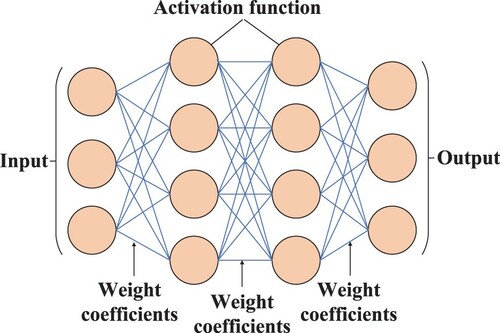
The ANN is a mathematical model that simulates the structure and the function of the biological neural networks, which consists of a large number of processing units connected with each other. Recently, the scholars have paid much attention to the ANN (J. Li, Dong, Wang, & Bu, 2020; J. Li, Dong, Wang, & Fei, 2020; J. Li et al., 2018). The ANN has the capability of self-learning and solving some problems such as classification and prediction (Bohorquez et al., 2020; Gunerkar et al., 2019; Laredo et al., 2019; Shaik et al., 2020; Sharma et al., 2019; Tavakoli et al., 2020). The specific structure of ANN is shown in Figure 8. The neurons are connected by certain weights, and the input is converted into the output through the activation function. Till now, the ANN has been successfully applied in faults classification for bearings (Gunerkar et al., 2019; Sharma et al., 2019) and pipelines (Bohorquez et al., 2020; Shaik et al., 2020; Tavakoli et al.,2020).

Figure 8. The structure of ANN.

It should be pointed out that ANN is frequently combined with other algorithms. In Gunerkar et al. (2019), aiming at classifying multiple faults of bearings, the fault features have been firstly extracted from the time-domain signals by WT. Then the features have been input into the ANN to classify the faults, and the obtained experiment results have verified that the ANN has a better classification accuracy than K-nearest neighbour algorithm in multiple faults classification problem. Towards the pipelines, the ANN based on the fluid transient waves has been adopted for leak detection of pipelines (Bohorquez et al., 2020). Whereafter, in Tavakoli et al. (2020), the wall thickness loss of the pipelines has been chosen as the health indicator. Then the ANN has been used to train the model for RUL prediction by combining the adaptive neural fuzzy inference system, in which a deterioration evaluation index has established for training. In Laredo et al. (2019), the combination of differential evolution algorithm and multi-layer perceptron has been conducted to predict the RUL of the mechanical system, in which the deterioration evaluation algorithm has been adopted to optimize the data-related parameters.

2.3.2. Support vector machine

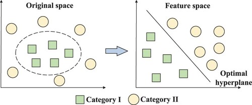
In the implementation of the ANN, the empirical components often play an important role, while the SVM has strict theory and mathematical basis. The SVM has been first proposed by Cortes and Vapnik (1995), which is a small sample data training and classification algorithm based on supervised learning. As is shown in Figure 9, the original space is generally a low-dimensional space such that it is difficult to achieve linear classification of samples. Consequently, some feature extraction methods have been proposed for extracting the typical features to obtain a feature space, and then an optimal hyperplane formed by the SVM has been achieved for linear classifications.

Figure 9. The illustration of basic SVM.

With the rapid developments of the intelligent optimization algorithms, some optimization algorithms have been applied in parameter optimizations of the SVM(Han et al., 2019; C. Wang, Han, Zhang, et al., 2020; C. Wang et al., 2019; D. Yang et al., 2015; Yao et al., 2018). In Han et al. (2019), the fault features of the gears under different load excitations have been extracted from different domains, respectively, thereby inputting into the PSO-SVM model sequentially to classify the faults of the gears. In the proposed method, the peak index of the SVM has been optimized by the PSO algorithm. As an extension of the PSO, the leader-follower PSO algorithm has been adopted to select the super-parameter C of the SVM in C. Wang, Han, Zhang, et al. (2020), which has constructed a new model to detect pipeline leakage. The discriminative and robust features of pipeline leakage data extracted by sparse autoencoder networks have been input into proposed model for further classification.

It has been observed from plenty of academic and industrial research that the research status of the SVM is similar to that of the ELM. In the field of FD, the research concerning the SVM has been roughly divided into two aspects, which includes the parameter optimization of the SVM and the signal preprocessing (Gangsar & Tiwari, 2017; Gong et al., 2019; Keskes & Braham, 2015; Z. Liu et al., 2017; R. Xiao et al., 2019; X. L. Zhang et al., 2015; J. D. Zheng et al., 2017). A multi-variable integrated incremental SVM has been shown in X. L. Zhang et al. (2015) for FD of rolling bearings. Specifically, the original signals have been extracted to form a number of multi-variable feature subsets, which have been input into the SVM model for the sake of obtaining the multi-faults classification results through ensemble and incremental learning. In R. Xiao et al. (2019), the WT and Release-F algorithm have been employed to select the most discriminative pipeline leakage features, which have been then input into the SVM classifier to identify the leakage severity of the pipelines. Furthermore, as one of the representatives of DL, CNN has also been combined with SVM to diagnose the incipient micro-faults of the Gong et al. (2019), in which the original data has been fed into the improved CNN-softmax model to extract features, and the sparse representatives of the features have been fed into SVM for fault classifications. The proposed method has higher diagnosis accuracy than the methods containing individual SVM, K-nearest neighbour and deep back propagation neural network.

2.3.3. Extreme learning machine

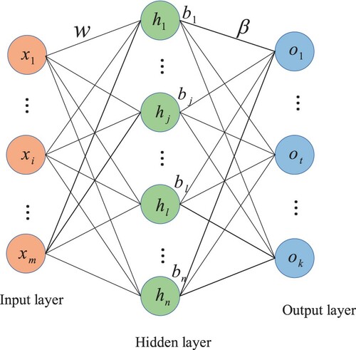
In essence, both the SVM and the ELM are used for classification in high-dimensional space through certain mapping. It is worth pointing out that the SVM is good at binary classification problem and the ELM is good at multi-classification problem. Compared with the SVM, the ELM has faster training speed (G. Huang et al., 2006). As is indicated in Figure 10, the ELM is a single hidden layer feed-forward neural network and only the number of the nodes in the hidden layer needs to be set, which exhibits fast learning speed and good generalization performance (G. Huang et al., 2015). It is worth noting that the parameter optimization methods and the distinctive feature representation methods have been combined with ELM frequently during the past decade (Jiang et al., 2019; Z. Wang et al., 2019). In Z. Wang et al. (2019), the FD of the bearings has been considered, in which a novel krill herd algorithm has been adopted to optimize the parameters of the ELM. Then the extracted feature vectors of the faults of the bearings have been imported into the kernel ELM for FD. In Jiang et al. (2019), the Mel-frequency cepstrum coefficient, as a signal feature representation method, has been combined with ELM for FD of pumps. The features of the denoised sound signals have been fed into the trained ELM model, which leads to the optimal number of the neurons in the hidden layer. The proposed method has higher recognition accuracy and shorter training and diagnosing time (Jiang et al., 2019).

Figure 10. The structure of ELM.

Recently, the combinations of ELM and signal preprocessing methods have stirred a great deal of attention (Z. Chen et al., 2019; X. Liu et al., 2020; Rinanto et al., 2016; H. Shao et al., 2018; Wei et al., 2016; X. Zhao et al., 2020). It should be noted that the ELM is often used as a classifier. In H. Shao et al. (2018), together with deep wavelet autoencoder, the ELM has achieved higher accuracy of bearing fault classification. Multiple wavelet autoencoders have been employed to construct deep wavelet autoencoder for the sake of enhancing the ability of unsupervised feature learning, which is capable of capturing the features of the signals effectively. Then the captured features have been input into the ELM model to identify different faults of the bearings. In Wei et al. (2016), the ELM has been applied to identifying and classifying faults of the gears by combining with the local mean decomposition method. Furthermore, in X. Liu et al. (2020), in order to identify the types of the faulty gears, the fault samples have been firstly obtained through establishing the finite element model of the gears. Then the measured vibration signals of the gear transmission system have been adopted to be the test samples, which are input into the trained ELM to realize fault identifications.

3. Methods based on deep learning

During the past decades, the FD and RUL prediction issues based on the SL have developed rapidly. Whereas in most cases, the SL needs prior knowledge and preprocessing technique before diagnosing faults and predicting the RUL, and the representation ability of the SL is limited as well. With the arrival of the big data era, it is difficult for SL to automatically process and analyse massive data. As such, as another significant branch of ML, DL has attracted many scholars' attention. On account of the strong ability of feature extraction, the DL has been successfully applied to the training of massive data.

In 2006, a theoretical breakthrough on DL has been achieved in terms of greedy learning algorithm (Hinton et al., 2006). Subsequently, DL has attracted tremendous research attention of the scholars who seek to solve the practical problems. Up to now, DL has been successfully applied in many engineering fields with examples including image recognition (Fujiyoshi et al., 2019; Mezgec & Seljak, 2017; Traore et al., 2018), speech recognition (Graves et al., 2013; Noda et al., 2015; B. Wu et al., 2017), FD (Jia et al., 2016; F. Li, Pang, et al., 2019; Y. Li, Cheng, et al., 2018; W. Sun et al., 2016; J. Wang et al., 2017, 2019; X. Zhao & Jia, 2019), RUL prediction (L. Guo et al., 2017; Hong et al., 2019; Ren et al., 2018; Zhu et al., 2019) and so on. In this part, a brief review of DL including DNN, DBN, CNN and RNN with their applications is given.

3.1. Deep neural networks

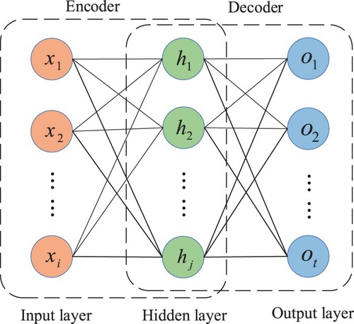
DNN is a kind of artificial neural networks where multiple hidden layers exist between the input layer the and output layer. It is claimed that the hidden layers are trained through massive data to improve the accuracy of clustering or prediction (Hong et al., 2019). DNN is a multi-layer neural network formed by the stack of multi-layer feature representation models which generally include autoencoders, stacked autoencoders (G. Liu et al., 2018; Tan et al., 2015; J. Wang et al., 2017), denoising autoencoders (Lu et al., 2017; Meng et al., 2018), sparse autoencoders (Z. Chen & Li, 2017; W. Sun et al., 2016; Wen et al., 2019) and so on. It can be seen from Figure 11 that the autoencoder mainly consists of an encoder and a decoder. The encoder is capable of mapping the input data from a high-dimensional space to a low-dimensional space and obtaining the feature representation of the input data. On the contrary, the decoder is capable of mapping the input data from a low-dimensional space to a high-dimensional space and reproducing the input.

Figure 11. The structure of autoencoder.

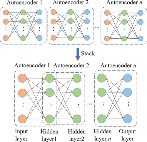
As is shown in Figure 12, stacking multiple autoencoders can form the stacked autoencoders, i.e. a DNN. In J. Wang et al. (2017), the stacked autoencoders have been utilized to extract features, which have been then adopted to train the softmax regression classifier to identify the faults of the gears. The stacked autoencoders have been combined with the wavelet soft threshold method and back propagation network for FD of the bearings as well (Tan et al., 2015). To be specific, the stacked autoencoders have been employed to extract the features of the fault vibration signals denoised by the wavelet soft threshold method, which have been regarded as the input of the back propagation network to train the model. Furthermore, as a technique to solve the over-fitting problem, dropout has been introduced into the stacked autoencoders (G. Liu et al., 2018). Together with the ReLU activation function, the method has been used to capture the salient features of the faulty gears.

Figure 12. The formation process of stacked autoencoders.

In the presence of noises, the robustness of the autoencoders is far from satisfactory, and thus the denoising autoencoders have been proposed to reduce the sensitivity to the noises. In Meng et al. (2018), with the addition of the regularization terms, the noise level has been decreased at the back layers so as to adapt the different robustness of the different layers. The improved method has shown a high accuracy in FD of rolling bearings. Moreover, in Lu et al. (2017), the denoising autoencoder has been combined with the stack for FD of the rotating machinery, which has shown good robustness in iterative learning.

On the basis of the traditional autoencoder, some sparse constraints have been introduced into the neurons in the hidden layer of the autoencoder to obtain the sparse autoencoder. In Z. Chen and Li (2017), the time- and frequency-domain features have been input into multiple two-layer sparse autoencoders for feature fusion. After that, the fused feature vectors, (i.e. the machine health indicators), have been fed into the DBN for further fault classification of rotating machine. Subsequently, breakthrough on three-layer sparse autoencoders has been achieved for FD of bearings in Wen et al. (2019), which has been adopted to extract the features of the original data. Meanwhile, the discrepancy penalty between the features of the training data and the test data has been minimized through applying the maximum mean discrepancy term, which leads to a higher diagnosis accuracy than ANN, SVM and so on. In W. Sun et al. (2016), to identify the faults of the induction motor, the partial corruption is added into the input of the sparse autoencoder by means of denoising coding so as to improve the robustness of the feature representation. The features learned from the sparse autoencoder are then used to train a neural network classifier for identifying the faults.

3.2. Deep belief networks

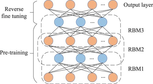
When it comes to DBN, the restricted Boltzmann machine (RBM) can not be ignored, which contains two layers, i.e. visible layer and hidden layer. It should be pointed out that the neurons in one layer are connected to all the neurons in the other layer, whereas there are no connections between the neurons in the same layer. The structure of RBM is shown in Figure 13. In order to solve the linear inseparable problem, Hinton et al. have proposed the DBN in 2006 (Hinton et al., 2006), which are composed of multiple RBMs as shown in Figure 14. The training process of DBN has been divided into two stages, the first one of which is pre-training. Specifically, the RBM has been trained by greedy training algorithm from the bottom to the top. Then the output of the current hidden layer has been regarded as the input of the next RBM, which has been repeated constantly. The parameters of the model have been transferred layer by layer and optimized continuously to achieve local optimum. The second stage is reverse fine-tuning. In the last layer of DBN, the back propagation algorithm has been employed to propagate the training error from the high layer to the low layer and fine-tune the whole DBN, which therefore achieves the global optimum.

Figure 13. The structure of RBM.

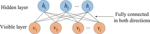
Figure 14. The structure of DBN.

It is widely recognized that the DBN has been successfully applied in the fields of leak detection, FD and so on (Y. Guo et al., 2019; W. Liu, Wang, Zeng, et al., 2021; S. Wang et al., 2018; Zeng et al., 2021). In recent years, the DBN has been utilized by combining other methods (H. Chen et al., 2016; J. Huang et al., 2019; Lang et al., 2018; J. Li, Li, et al., 2020; Zhu et al., 2020). For example, in Zhu et al. (2020), the principal component analysis has been implemented to reduce the dimension of the original vibration bearing signals and then the fault features have been extracted according to primary eigenvalues and eigenvectors, which have been input into the DBN model. As another well-known signal preprocessing method, the wavelet packet analysis has been adopted to remove the noise in Lang et al. (2018), and then the denoised signals have been fed into the DBN with independent component regression to recognize different leak apertures. It should be noted that the classification accuracy has been improved when using independent component regression instead of the traditional gradient fine-tuning in the DBN.

It is crucial to optimize the parameters in the DBN. Some recent advances in the field of parameter optimization have stirred a great deal of attention (Gai et al., 2020; He et al., 2017; K. Yu et al., 2020). In K. Yu et al. (2020), the combination of hybrid genetic algorithm (GA) and PSO has been employed to optimize the parameter of DBN for the classifications of the states and severities of the bearing faults. Next, combining with the dempster-shafer theory, the classification results of DBN have been further fused and hence the FD accuracy has been improved. It is worth noting that the GA has also been adopted to optimize the parameters of the DBN in He et al. (2017). With less requirement on prior knowledge, the GA-DBN model has adaptively utilized the robust features related to the faults and achieved the unsupervised FD of the gear transmission chain. Moreover, in order to diagnose the faults of gears more accurately, the learning rate and batch learning number with a great influence on the training error of DBN have been optimized in Gai et al. (2020). The above mentioned methods have solved the weakness of the generalization ability of the single classifier under the big data environment.

Recently, much attention has been devoted to improving the internal structure of the DBN so as to improve the performance (Che et al., 2020; Qin et al., 2019; Yan, Liu, & Jia, 2020; T. Zhang et al., 2019). For instance, a method based on domain adaptive DBN has been proposed for FD of rolling bearings in Che et al. (2020). To be specific, the domain adaptive method has been used to calculate the discrepancy of the multi-kernel maximum mean in the last two hidden layers, which has been introduced into the loss function to fine-tune the model parameters so as to improve the generalization ability of the model. In addition, the activation function of the DBN in FD of the gearboxes has been improved in Qin et al. (2019) and the traditional Sigmoid function has been replaced by the improved logistic Sigmoid (Isigmoid) function, which has overcome the gradient vanishing problem in the process of back propagation. Furthermore, a multi-scale cascading DBN has been constructed for the automatic fault identification of the rotating machinery in Yan, Liu, and Jia (2020), which can not only directly learn the high-level feature representation from the multi-scale features, but also automatically identify the faults through cascading and softmax classifier.

3.3. Convolution neural networks

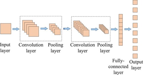
As a kind of neural networks, CNN has become a research hotspot in the field of ML, the basic structure of which has been composed of input layer, convolution layer, pooling layer, fully-connected layer and output layer as shown in Figure 15.

Figure 15. The structure of CNN.

It should be pointed out that the one-dimensional (1-D) CNN is capable of processing time series data. With this property, the 1-D CNN has been widely applied in FD and RUL prediction during the past decade (Ince et al., 2016; C. Wu et al., 2019). In C. Wu et al. (2019), the relationship between the convolution kernel length and the accuracy has been obtained, and the number of layers has been determined by checking the distribution of the weight vector. Similarly, the constructed 1-D CNN has been employed for FD of the gearboxes.

The two-dimensional (2-D) CNN has been viewed as a significant technique to solve the image problems. In the past decade, it is found that 2-D CNN has more applications in the fields of FD and RUL prediction than the 1-D one (Grezmaka et al., 2019; S. Guo et al., 2020; T. Li et al., 2020; S. Shao et al., 2020; F. Wang et al., 2021; Wen et al., 2018; Xie et al., 2020; B. Yang et al., 2019; Zhu et al., 2019). For example, in Grezmaka et al. (2019), the layer-wise relevance propagation that is adopted to explain the correlation between the time-frequency spectrum and the fault types has been introduced into the 2-D CNN to diagnose the faults of the gearboxes, in which the WT has been firstly adopted to convert the vibration signals into time-frequency spectra images, and then input into the CNN to achieve the fault classification. In T. Li et al. (2020), a multi-scale multi-sensor feature fusion CNN has been proposed to extract the signal features with different scales and the information fusion has been performed on the data and feature level. The proposed method has a higher accuracy and faster convergence speed than the standard CNN in the gear fault detection.

In F. Wang et al. (2021), a cascade structure has been established in the CNN for FD of motors, which has avoided the information loss caused by the consecutive convolution striding or pooling. In addition, a divide-and-conquer parameters optimization algorithm has been used to make the cascade CNN converge to a better state, which has improved the diagnosis performance. As well as RUL prediction, two CNNs have been combined to predict the RUL of bearings. The incipient failure points have been identified by one CNN and then the RUL has been predicted by the other one. It is worth mentioning that an intermediate reliability variable has been mapped to RUL by a proposed mapping algorithm, which has achieved higher prediction accuracy and better robustness than other methods (B. Yang et al., 2019). Furthermore, the combination of multi-scale CNN and time-frequency representation has been proposed to predict the RUL of bearings in Zhu et al. (2019). In this method, the WT has been adopted to obtain the time-frequency representation containing a lot of useful information, which has been then given to the multi-scale CNN that is capable of keeping the global and local information synchronously and learning the significant features automatically.

3.4. Recurrent neural networks

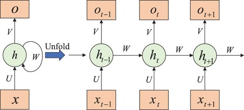
With the developments of artificial intelligence, the research on RNN has sprung up gradually. The Jordan network (Jordan, 1986) in 1986 and the Elman network (Elman, 1990) in 1990 have been regarded as the earliest RNN. The RNN takes the sequence data as the input and performs the recursion in the direction of the sequence. Additionally, all the recurrent units are connected by chains. As shown in Figure 16, the value of the hidden layer not only depends on the current input, but also relies on the previous hidden layer. Consequently, it is suitable for RNN to deal with the time series data.

Figure 16. The structure of RNN.

The applications of RNN and its variants in the fields of FD and RUL prediction have been increasing in recent years (L. Guo et al., 2017; F. Li, Chen, et al., 2019; H. Liu et al., 2018; Y. Peng et al., 2017; J. Yu et al., 2019). In F. Li, Chen, et al. (2019), a reinforcement learning unit matching RNN has been proposed to predict the degradation tendency of the rolling bearing. Specifically, the moving average singular spectral entropy has been selected as the state degradation feature of the rolling bearing, which has been input into the reinforcement learning unit matching RNN to complete the trend prediction of the rolling bearing states. Meanwhile, there are also some indicators established in L. Guo et al. (2017) such as the bearing RUL prediction indicator based on RNN. In Y. Peng et al. (2017), a RNN-based fault prediction method has been proposed for the gearbox, where the health index extracted from the generator current signal has been employed to quantify the health state of the gearbox. In the proposed method, the RNN has been established and trained by using the real time recurrent learning algorithm online to predict the health state.

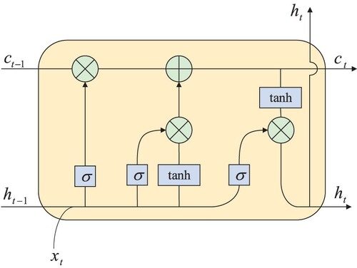
The above discussions have verified that the RNN has successfully applied in many fields. Nevertheless, the RNN is prone to the problems of gradient explosion and gradient disappearance in the process of training and thus the gradient cannot be transmitted in longer sequence. In order to solve the gradient disappearance problem of RNN, some variants of RNN such as long short-term memory (LSTM) (Hochreiter & Schmidhuber, 1997) have stirred much research attention in recent years. The LSTM has the memory unit and gate unit as shown in Figure 17. It should be noted that there are three types of gates in the LSTM, in which the forgetting gate controls the number of the information that can be transmitted from the previous unit to the current unit, and the input gate controls the number of the input information that can be saved in the current unit. Additionally, the output gate controls the number of the information that the current unit can output.

Figure 17. The structure of LSTM.

During the past decade, many research groups throughout the world from not only academia but also industry have been motivated to apply the LSTM to the field of FD (An et al., 2020; D. Xiao et al., 2019; Ye et al., 2020; Yin et al., 2020). For example, an intelligent FD framework of the bearing based on LSTM has been proposed in An et al. (2020), in which the sample has been firstly segmented, and then each segment dimension of the sample has been extended by the input network with the hope of ensuring that there is adequate information memory space. Then the classification information has been stored and transferred in the LSTM network such that the health states can be classified by the output network. It should be noted that the LSTM has also been combined with other methods frequently. In D. Xiao et al. (2019), the recurrence quantification analysis features extracted from the recurrence plots and the empirical statistical features extracted from the time- and frequency-domain have been combined with the features extracted by the LSTM for constructing a hybrid feature set. Then the combined features have been input into a weighted batch normalization block. Finally, the faults have been diagnosed through a three-layer fully connected neural network. Additionally, the optimization of LSTM has attracted much research attention. For instance, in Yin et al. (2020), an optimized LSTM network with cosine loss (Cos-LSTM) has been established to diagnose the faults of gearboxes. In practice, the cosine loss is critical to eliminating the influence of signal strength and improving the diagnosis accuracy. Especially, the cosine loss is capable of converting the loss from the Euclid space to the angular space. The energy sequence features and wavelet energy entropy have been introduced into the Cos-LSTM networks such that the diagnosis accuracy of the Cos-LSTM is higher than those of other classical methods.

Compared with the DNN, the DBN is more competitive in dealing with the unlabeled classification problem. As for the high-dimensional data, the CNN combining the parameter sharing mechanism is commonly employed to reduce the computational complexity such that the classification problem of the high-dimensional data, e.g. the image, can be solved effectively. In addition, for time-dependent problem, it is difficult for the DNN to capture the temporal relationships. Therefore, much effort has been devoted to the RNN owing to its advantages in dealing with the time-dependent problem, where the value of the current hidden layer not only relies on the value of the current input, but also depends on the value of the previous hidden layers.

4. Conclusion

In this paper, we have reviewed the latest research progress based on the FD and RUL prediction. The structures and applications in FD and RUL prediction of PME based on MS and ML are investigated, in which the applications based on DL are summarized more specifically. The discussed methods in this review and the corresponding references are summarized in the following Table 1. Inspired by the above literature review, some critical and unresolved main issues in the future are listed as follows.

Table 1. Summary of FD and RUL prediction of PME.

Methods	References
STFT	bearings (H. Li et al., 2019; Y. Zhang et al., 2020); gears (Bian et al., 2019); pumps (W. Zhao et al., 2016)
WT	bearings (Islam & Kim, 2019; Wan & Zhang, 2018); gears (Ahuja et al., 2020; Bajric et al., 2016; R. Chen et al., 2019; Liang et al., 2019; Parey & Singh, 2019; L. Wang, Liu, et al., 2020); pumps (H. Yu et al., 2020; Z. Zheng et al., 2019); others (Kordestani et al., 2018; X. Zhang et al., 2019)
EMD	bearings (Abdelkader et al., 2016, 2018; Cheng et al., 2019; L. Wang & Shao, 2020; Xue et al., 2015); gears (Park et al., 2018); motors (Karatoprak & Seker, 2019); pumps (Alabied et al., 2018; Y. Wang, Zhu, et al., 2020); pipelines (C. Guo et al., 2016; Xu et al., 2020)
VMD	bearings (Z. Li et al., 2018; Miao et al., 2019; X. Zhang et al., 2018); gears (Y. Li, Li, et al., 2018; X. Zhang et al., 2018); motors (Z. Guo et al., 2019); pumps (Y. Chen et al., 2019); pipelines (Diao et al., 2020; Ju et al., 2019); others (Yan, Liu, Zhang, et al., 2020; S. Zhao et al., 2020; D. Zou & Ge, 2019)
KF	bearings (Cui et al., 2020, 2019; Singleton et al., 2015); gears (Z. Feng et al., 2019; Y. Li et al., 2019); motors (Kandukuri et al., 2019; Naseri et al., 2020); pipelines (Moulahi & Hmida, 2020); others (Asl et al., 2019; Naseri et al., 2020)
PF	bearings (C. Chen et al., 2011; Lei, Li, Gontarz, et al., 2016; Lei, Li, & Lin, 2016; Qian & Yan, 2015); gears (C. Chen et al., 2012; L. Yang & Chen, 2019); others (K. Peng et al., 2019; J. Yu, 2015; Zio & Peloni, 2011)
ANNs	bearings (Gunerkar et al., 2019; Sharma et al., 2019); pipelines (Bohorquez et al., 2020; Shaik et al., 2020; Tavakoli et al., 2020); others (Laredo et al., 2019)
ELM	bearings (H. Shao et al., 2018; Z. Wang et al., 2019); gears (Z. Chen et al., 2019; X. Liu et al., 2020; Wei et al., 2016); pumps (Jiang et al., 2019); others (Rinanto et al., 2016; X. Zhao et al., 2020)
SVM	bearings (Gong et al., 2019; Z. Liu et al., 2017; Yao et al., 2018; X. L. Zhang et al., 2015; J. D. Zheng et al., 2017); gears (Han et al., 2019; Z. Liu et al., 2017; D. Yang et al., 2015); motors (Gangsar & Tiwari, 2017; Keskes & Braham, 2015); pipelines (C. Wang, Han, Zhang, et al., 2020; R. Xiao et al., 2019)
DNN	bearings (Z. Chen & Li, 2017; Jia et al., 2016; Lu et al., 2017; Meng et al., 2018; Ren et al., 2018; Tan et al., 2015; J. Wang et al., 2019; Wen et al., 2019; X. Zhao & Jia, 2019); gears (Jia et al., 2016; F. Li, Pang, et al., 2019; Y. Li, Cheng, et al., 2018; G. Liu et al., 2018; J. Wang et al., 2017, 2019; X. Zhao & Jia, 2019);
	motors (W. Sun et al., 2016); pipelines (Zadkarami et al.,2020)
DBN	bearings (Che et al., 2020; J. Li, Li, et al., 2020; Yan, Liu, & Jia, 2020; K. Yu et al., 2020; Zhu et al., 2020); gears (H. Chen et al., 2016; Gai et al., 2020; He et al., 2017; J. Li, Li, et al., 2020; Qin et al., 2019; Yan, Liu, & Jia, 2020); pumps (S. Wang et al., 2018); pipelines (Y. Guo et al., 2019);
	others (J. Huang et al., 2019; Lang et al., 2018; T. Zhang et al., 2019)
CNN	bearings (S. Guo et al., 2020; Wen et al., 2018; B. Yang et al., 2019; Zhu et al., 2019); gears (Grezmaka et al., 2019; T. Li et al., 2020; C. Wu et al., 2019); motors (Ince et al., 2016; S. Shao et al., 2020; F. Wang et al., 2021); pumps (Wen et al., 2018); pipelines (Xie et al., 2020)
RNN	bearings (An et al., 2020; L. Guo et al., 2017; F. Li, Chen, et al., 2019; H. Liu et al., 2018); gears (Y. Peng et al., 2017; Yin et al., 2020; J. Yu et al., 2019); motors (D. Xiao et al., 2019); others (Ye et al., 2020)

1. How to deal with the poor-quality data of the PME. Owing to the influence of the environment and the abnormality of the sensors and the data transmissions, the abnormal, missing and repeated data may occur which will affect the accuracy of the FD and RUL prediction. As such, we should further develop effective methods to alleviate the influence of the poor-quality data.

2. How to address the feature correlation and the data limitation in data space. The feature dimension of the data space is always high, and thus it is difficult to distinguish the strong correlation between the features such as the feature correlation of the FD. As another disadvantage that cannot be ignored is that the data category is unbalanced because the equipments always work under normal conditions for getting normal data, therefore, the number of the fault sample data is limited. At present, to the best of our knowledge, the methods to deal with these problems are still at the early stage.

3. How to solve the mismatch problem of the data collected by multiple sensors. Different sensors exhibit different sensitivities to the PME, which may lead to the mismatch problem of the collected data, thereby resulting in different data transfer rates. That is to say, if the multi-rate data collected by multiple sensors does not match each other, the difficulties of FD and RUL prediction will increase dramatically. Therefore, the research on multi-sensor information fusion is also a problem to be considered.

4. How to suppress the noise and decompose the components of the main features of the signals in FD. In reality, the signals to be decomposed are usually consisted of the noise and the disturbance which are not related to the desired features of the signals, and thus the important fault features cannot be found in time. In addition, the expected signals are usually relatively weak and easy to be drowned by noise/disturbance (M. Wang et al., 2021). Consequently, more research should be conducted on suppressing the noise/disturbance so as to improve the resolution and the robustness of the decomposition method.

5. How to distinguish the multiple faults. In general, there may be multiple faults in a single component, and thus how to distinguish them and take measures to settle them should be considered adequately.

For the above problems, the corresponding suggestions are provided for readers to study.

1. Establish a standard big database of the PME. First of all, a unified measurement standard of the data quality should be constructed, and then the test data of the experimental platform and the long-term monitoring data of PME should be shared with each other such that the data deficiencies are made up. In addition, some data cleaning methods such as the spatial clustering algorithm can be adopted to clean the abnormal data. Some methods conducive to data transmission can also be introduced, such as coding-decoding communication protocol (L. Wang et al., 2019). Moreover, more attention should be paid to the research of multi-scale and dimension conversion so as to provide high-quality data for training diagnostic models based on ML.

2. Increase the capacity of the data. For the problem of small samples with limited data, the methods of under-sampling, over-sampling, cost-sensitive learning and unbalanced learning may be employed to preprocess the data for solving the uneven distribution of data categories. Meanwhile, the flow information, transfer learning, generative adversarial networks (GAN) (Goodfellow et al., 2014; W. Liu, Wang, Tian, et al., 2021) and other methods should be tried to enhance the depth and breadth of the data.

3. Focus on the developments of data fusion model. The unified data fusion framework may be established including the general process of data processing, the unified model structure of data fusion space, the fusion results of data normalization and so on. Furthermore, the heterogeneous information should be preprocessed such as the unified representation, conversion and de-heterogeneity. Then the multi-dimensional information should be calibrated and spatiotemporal matched for maintaining the consistency of multi-sensor data information and ensuring the effects of data fusion.

4. Develop the denoising methods. With the rapid developments of the signal processing, the denoising methods are becoming more and more mature. A variety of denoising methods may be combined with the purpose of complementing the advantages and disadvantages of each method and achieving a better denoising result. In addition, the anti-interference technologies such as spatial filtering (Wong et al., 2020; D. Wu et al., 2018) and space-time adaptive filtering (Blunt et al., 2017) may be employed to improve the anti-interference ability of the PME signals.

5. Determine the types of the faults. The law of the effects of different faults on the life degradations of the PME components should be studied, and a hybrid model of component failure and RUL should be established as well. According to the model, the ranges of the faults will be judged and thus the types of the faults can be determined.

Disclosure statement

No potential conflict of interest was reported by the author(s).

Additional information

Funding

This work was supported in part by the National Natural Science Foundation of China under Grants 61873058 and 61933007.

References

- Abdelkader, R., Derouiche, Z., Kaddour, A., & Zergoug, M. (2016). Rolling bearing faults diagnosis based on empirical mode decomposition: Optimized threshold de-noising method. In 2016 8th International conference on modelling, identification and control (ICMIC) (pp. 186–191). IEEE.
- Abdelkader, R., Kaddour, A., Bendiabdellah, A., & Derouiche, Z. (2018). Rolling bearing fault diagnosis based on an improved denoising method using the complete ensemble empirical mode decomposition and the optimized thresholding operation. IEEE Sensors Journal, 18(17), 7166–7172. https://doi.org/https://doi.org/10.1109/JSEN.7361
- Ahuja, A. S., Ramteke, D. S., & Parey, A. (2020). Vibration-based fault diagnosis of a bevel and spur gearbox using continuous wavelet transform and adaptive neuro-fuzzy inference system. Soft Computing in Condition Monitoring and Diagnostics of Electrical and Mechanical Systems, 1096, 473–496. https://doi.org/https://doi.org/10.1007/978-981-15-1532-3
- Alabied, S., Haba, U., Daraz, A., Gu, F., & Ball, A. D. (2018). Empirical mode decomposition of motor current signatures for centrifugal pump diagnostics. In 2018 24th International conference on automation and computing (ICAC) (pp. 1–6). IEEE.
- Alves, M. V. C., Barbosa, J. R., Prata, A. T., & Ribas, F. A. (2011). Fluid flow in a screw pump oil supply system for reciprocating compressors. International Journal of Refrigeration, 34(1), 74–83. https://doi.org/https://doi.org/10.1016/j.ijrefrig.2010.08.003
- An, Z., Li, S., Wang, J., & Jiang, X. (2020). A novel bearing intelligent fault diagnosis framework under time-varying working conditions using recurrent neural network. ISA Transactions, 100, 155–170. https://doi.org/https://doi.org/10.1016/j.isatra.2019.11.010
- Arulampalam, M. S., Maskell, S., Gordon, N., & Clapp, T. (2002). A tutorial on particle filters for online nonlinear/non-Gaussian Bayesian tracking. IEEE Transactions on Signal Processing, 50(2), 174–188. https://doi.org/https://doi.org/10.1109/78.978374
- Asl, R. M., Hagh, Y. S., Simani, S., & Handroos, H. (2019). Adaptive square-root unscented Kalman filter: An experimental study of hydraulic actuator state estimation. Mechanical Systems and Signal Processing, 132, 670–691. https://doi.org/https://doi.org/10.1016/j.ymssp.2019.07.021
- Aziz, S., Khan, M. U., Aamir, F., & Javid, M. A. (2019). Electromyography (EMG) data-driven load classification using empirical mode decomposition and feature analysis. In 2019 International conference on frontiers of information technology (FIT) (pp. 272–2725). IEEE.
- Bajric, R., Zuber, N., Skrimpas, G. A., & Mijatovic, N. (2016). Feature extraction using discrete wavelet transform for gear fault diagnosis of wind turbine gearbox. Shock and Vibration, 2016, Article ID 6748469. https://doi.org/https://doi.org/10.1155/2016/6748469
- Bian, J., Liu, X., & Xu, X. (2019). Gearbox fault diagnosis method based on deep convolutional neural network vibration signal image recognition. In 2019 14th IEEE international conference on electronic measurement and instruments (ICEMI) (pp. 456–465) . IEEE.
- Blunt, S. D., Metcalf, J., Jakabosky, J., Stiles, J., & Himed, B. (2017). Multi-waveform space-time adaptive processing. IEEE Transactions on Aerospace and Electronic Systems, 53(1), 385–404. https://doi.org/https://doi.org/10.1109/TAES.2017.2650639
- Bohorquez, J., Alexander, B., Simpson, A. R., & Lambert, M. F. (2020). Leak detection and topology identification in pipelines using fluid transients and artificial neural networks. Journal of Water Resources Planning and Management, 146(6), 04020040. https://doi.org/https://doi.org/10.1061/(ASCE)WR.1943-5452.0001187.
- Carpenter, J., Clifford, P., & Fearnhead, P. (1999). Improved particle filter for nonlinear problems. IEE Proceedings – Radar, Sonar and Navigation, 146(1), 2–7. https://doi.org/https://doi.org/10.1049/ip-rsn:19990255
- Che, C., Wang, H., Ni, X., & Fu, Q. (2020). Domain adaptive deep belief network for rolling bearing fault diagnosis. Computers and Industrial Engineering, 143, Article 106427. https://doi.org/https://doi.org/10.1016/j.cie.2020.106427
- Chen, C., Vachtsevanos, G., & Orchard, M. E. (2012). Machine remaining useful life prediction: An integrated adaptive neuro-fuzzy and high-order particle filtering approach. Mechanical Systems and Signal Processing, 28, 597–607. https://doi.org/https://doi.org/10.1016/j.ymssp.2011.10.009
- Chen, C., Zhang, B., Vachtsevanos, G., & Orchard, M. (2011). Machine condition prediction based on adaptive neuro-fuzzy and high-order particle filtering. IEEE Transactions on Industrial Electronics, 58(9), 4353–4364. https://doi.org/https://doi.org/10.1109/TIE.2010.2098369
- Chen, H., Wang, J., Tang, B., Xiao, K., & Li, J. (2016). An integrated approach to planetary gearbox fault diagnosis using deep belief networks. Measurement Science and Technology, 28(2), 025010.
- Chen, J., Li, Z., Pan, J., Chen, G., Zi, Y., Yuan, J., Chen, B., & He, Z. (2016). Wavelet transform based on inner product in fault diagnosis of rotating machinery: A review. Mechanical Systems and Signal Processing, 70–71, 1–35. https://doi.org/https://doi.org/10.1016/j.ymssp.2015.08.023
- Chen, R., Huang, X., Yang, L., Xu, X., Zhang, X., & Zhang, Y. (2019). Intelligent fault diagnosis method of planetary gearboxes based on convolution neural network and discrete wavelet transform. Computers in Industry, 106, 48–59. https://doi.org/https://doi.org/10.1016/j.compind.2018.11.003
- Chen, Y., Huang, G., & Feng, Z. (2019). Early fault diagnosis of high pressure diaphragm pump check valve based on VMD-HMM. In 2019 IEEE 8th data driven control and learning systems conference (DDCLS) (pp. 808–813). IEEE.
- Chen, Z., Gryllias, K., & Li, W. (2019). Mechanical fault diagnosis using convolutional neural networks and extreme learning machine. Mechanical Systems and Signal Processing, 133, Article 106272. https://doi.org/https://doi.org/10.1016/j.ymssp.2019.106272
- Chen, Z., & Li, W. (2017). Multisensor feature fusion for bearing fault diagnosis using sparse autoencoder and deep belief network. IEEE Transactions on Instrumentation and Measurement, 66(7), 1693–1702. https://doi.org/https://doi.org/10.1109/TIM.2017.2669947
- Cheng, Y., Wang, Z., Chen, B., Zhang, W., & Huang, G. (2019). An improved complementary ensemble empirical mode decomposition with adaptive noise and its application to rolling element bearing fault diagnosis. ISA Transactions, 91, 218–234. https://doi.org/https://doi.org/10.1016/j.isatra.2019.01.038
- Choi, G., Oh, H., & Kim, D. (2018). Enhancement of variational mode decomposition with missing values. Signal Process, 142, 75–86. https://doi.org/https://doi.org/10.1016/j.sigpro.2017.07.007
- Cortes, C., & Vapnik, V. (1995). Support-vector networks. Machine Learning, 20(3), 273–297.
- Cui, L., Wang, X., Wang, H., & Ma, J. (2020). Research on remaining useful life prediction of rolling element bearings based on time-varying Kalman filter. IEEE Transactions on Instrumentation and Measurement, 69(6), 2858–2867. https://doi.org/https://doi.org/10.1109/TIM.19
- Cui, L., Wang, X., Xu, Y. G., Jiang, H., & Zhou, J. P. (2019). A novel switching unscented Kalman filter method for remaining useful life prediction of rolling bearing. Measurement, 135, 678–684. https://doi.org/https://doi.org/10.1016/j.measurement.2018.12.028
- Dai, C., Luo, G., & Long, Z. (2017). A signal process algorithm of relative position detection sensor for high speed maglev trains based on KF-UKF. In IEEE international conference on signal processing, communications and computing (ICSPCC) (pp. 1–6). IEEE.
- Das, K., Nath, D., & Pradhan, S. N. (2020). FPGA and ASIC realisation of EMD algorithm for real-time signal processing. IET Circuits, Devices and Systems, 14(6), 741–749. https://doi.org/https://doi.org/10.1049/cds2.v14.6
- Daubechies, I. (1990). The wavelet transform, time-frequency localization and signal analysis. IEEE Transactions on Information Theory, 36(5), 961–1005. https://doi.org/https://doi.org/10.1109/18.57199
- Diao, X., Jiang, J., Shen, G., Chi, Z., Wang, Z., Ni, L., Mebarki, A., Bian, H., & Hao, Y. (2020). An improved variational mode decomposition method based on particle swarm optimization for leak detection of liquid pipelines. Mechanical Systems and Signal Processing, 143, Article 106787. https://doi.org/https://doi.org/10.1016/j.ymssp.2020.106787
- Ding, D., Han, Q. L., Wang, Z., & Ge, X. (2019). A survey on model-based distributed control and filtering for industrial cyber-physical systems. IEEE Transactions on Industrial Informatics, 15(5), 2483–2499. https://doi.org/https://doi.org/10.1109/TII.9424
- Ding, D., Wang, Z., & Han, Q. (2020). A set-membership approach to event-triggered filtering for general nonlinear systems over sensor networks. IEEE Transactions on Automatic Control, 65(4), 1792–1799. https://doi.org/https://doi.org/10.1109/TAC.9
- Dragomiretskiy, K., & Zosso, D. (2014). Variational mode decomposition. IEEE Transactions on Signal Processing, 62(3), 531–544. https://doi.org/https://doi.org/10.1109/TSP.2013.2288675
- Elman, J. L. (1990). Finding structure in time. Cognitive Science, 14(2), 179–211. https://doi.org/https://doi.org/10.1207/s15516709cog1402_1
- Elsayed, W. T., Hegazy, Y. G., El-bages, M. S., & Bendary, F. M. (2017). Improved random drift particle swarm optimization with self-adaptive mechanism for solving the power economic dispatch problem. IEEE Transactions on Industrial Informatics, 13(3), 1017–1026. https://doi.org/https://doi.org/10.1109/TII.2017.2695122
- Feng, J., Lei, Y., Guo, L., Lin, J., & Xing, S. (2018). A neural network constructed by deep learning technique and its application to intelligent fault diagnosis of machines. Neurocomputing, 272, 619–628. https://doi.org/https://doi.org/10.1016/j.neucom.2017.07.032
- Feng, Z., Zhu, W., & Zhang, D. (2019). Time-frequency demodulation analysis via vold-Kalman filter for wind turbine planetary gearbox fault diagnosis under nonstationary speeds. Mechanical Systems and Signal Processing, 128, 93–109. https://doi.org/https://doi.org/10.1016/j.ymssp.2019.03.036
- Fujiyoshi, H., Hirakawa, T., & Yamashita, T. (2019). Deep learning-based image recognition for autonomous driving. IATSS Research, 43(4), 244–252. https://doi.org/https://doi.org/10.1016/j.iatssr.2019.11.008
- Gabor, D. (1946). Theory of communication. Part 1: The analysis of information. Journal of the Institution of Electrical Engineers – Part III: Radio and Communication Engineering, 93(26), 429–441.
- Gai, J., Shen, J., Wang, H., & Hu, Y. (2020). A parameter-optimized DBN using GOA and its application in fault diagnosis of gearbox. Shock and Vibration, 2020. Article ID: 4294095. https://doi.org/https://doi.org/10.1155/2020/4294095
- Gangsar, P., & Tiwari, R. (2017). Comparative investigation of vibration and current monitoring for prediction of mechanical and electrical faults in induction motor based on multiclass-support vector machine algorithms. Mechanical Systems and Signal Processing, 94, 464–481. https://doi.org/https://doi.org/10.1016/j.ymssp.2017.03.016
- Ge, X., Han, Q.-L., & Wang, Z. (2019). A threshold-parameter-dependent approach to designing distributed event-triggered H∞ consensus filters over sensor networks. IEEE Transactions on Cybernetics, 49(4), 1148–1159. https://doi.org/https://doi.org/10.1109/TCYB.6221036
- Georg, H., & Matthias, R. (2018). Deep learning for fault detection in wind turbines. Renewable and Sustainable Energy Reviews, 98, 189–198. https://doi.org/https://doi.org/10.1016/j.rser.2018.09.012
- Gong, W., Chen, H., Zhang, Z., Zhang, M., Wang, R., Guan, C., & Wang, Q. (2019). A novel deep learning method for intelligent fault diagnosis of rotating machinery based on improved CNN-SVM and multichannel data fusion. Sensors, 19(7), 1693. https://doi.org/https://doi.org/10.3390/s19071693.
- Goodfellow, I. J., Pouget-Abadie, J., Mirza, M., Xu, B., Warde-Farley, D., Ozair, S., Courville, A., & Bengio, Y. (2014). Generative adversarial nets. In Proceedings of the advances in neural information proceeding systems (pp. 2672–2680). MIT Press.
- Graves, A., Mohamed, A., & Hinton, G. (2013). Speech recognition with deep recurrent neural networks. In 2013 IEEE international conference on acoustics, speech and signal processing (pp. 6645–6649). IEEE.
- Grezmaka, J., Wang, P., Sun, C., & Gao, R. X. (2019). Explainable convolutional neural network for gearbox fault diagnosis. Procedia CIRP, 80, 476–481. https://doi.org/https://doi.org/10.1016/j.procir.2018.12.008
- Gu, J., Wang, Z., Kuen, J., Ma, L., Shahroudy, A., Shuai, B., Liu, T., Wang, X., Wang, G., Cai, J., & Chen, T. (2018). Recent advances in convolutional neural networks. Pattern Recognition, 77, 354–377. https://doi.org/https://doi.org/10.1016/j.patcog.2017.10.013
- Gunerkar, R. S., Jalan, A. K., & Belgamwar, S. U. (2019). Fault diagnosis of rolling element bearing based on artificial neural network. Journal of Mechanical Science and Technology, 33(2), 505–511. https://doi.org/https://doi.org/10.1007/s12206-019-0103-x
- Guo, C., Wen, Y., Li, P., & Wen, J. (2016). Adaptive noise cancellation based on EMD in water-supply pipeline leak detection. Measurement, 79, 188–197. https://doi.org/https://doi.org/10.1016/j.measurement.2015.09.048
- Guo, L., Li, N., Jia, F., Lei, Y., & Lin, J. (2017). A recurrent neural network based health indicator for remaining useful life prediction of bearings. Neurocomputing, 240, 98–109. https://doi.org/https://doi.org/10.1016/j.neucom.2017.02.045
- Guo, S., Zhang, B., Yang, T., Lyu, D., & Gao, W. (2020). Multitask convolutional neural network with information fusion for bearing fault diagnosis and localization. IEEE Transactions on Industrial Electronics, 67(9), 8005–8015. https://doi.org/https://doi.org/10.1109/TIE.41
- Guo, Y., Fan, Q., & Liu, X. (2019). Research on leakage diagnosis of heating pipe network based on deep belief network. In 2019 IEEE international conference on industrial internet (ICII) (pp. 303–304). IEEE.
- Guo, Z., Liu, M., Qin, H., & Li, B. (2019). Mechanical fault diagnosis of a DC motor utilizing united variational mode decomposition, SampEn, and random forest-SPRINT algorithm classifiers. Entropy, 21(5), 470. https://doi.org/https://doi.org/10.3390/e21050470
- Han, D., Zhao, N., & Shi, P. (2019). Gear fault feature extraction and diagnosis method under different load excitation based on EMD, PSO-SVM and fractal box dimension. Journal of Mechanical Science and Technology, 33(2), 487–494. https://doi.org/https://doi.org/10.1007/s12206-019-0101-z
- He, J., Yang, S., & Gan, C. (2017). Unsupervised fault diagnosis of a gear transmission chain using a deep belief network. Sensors, 17(7), 1564. https://doi.org/https://doi.org/10.3390/s17071564
- Heng, A., Zhang, S., Tan, A. C. C., & Mathew, J. (2009). Rotating machinery prognostics: State of the art, challenges and opportunities. Mechanical Systems and Signal Processing, 23(3), 724–739. https://doi.org/https://doi.org/10.1016/j.ymssp.2008.06.009
- Hinton, G. E., Osindero, S., & Teh, Y. W. (2006). A fast learning algorithm for deep belief nets. Neural Computation, 18(7), 1527–1554. https://doi.org/https://doi.org/10.1162/neco.2006.18.7.1527
- Hochreiter, S., & Schmidhuber, J. (1997). Long short-term memory. Neural Computation, 9(8), 1735–1780. https://doi.org/https://doi.org/10.1162/neco.1997.9.8.1735
- Hong, P., Hu, C., Si, X., Zhang, J., Pang, Z., & Zhang, P. (2019). Review of machine learning based remaining useful life prediction methods for equipment. Journal of Mechanical Engineering, 55(8), 1–13.
- Hu, J., Wang, Z., Alsaadi, F. E., & Hayat, T. (2017). Event-based filtering for time-varying nonlinear systems subject to multiple missing measurements with uncertain missing probabilities. Information Fusion, 38, 74–83. https://doi.org/https://doi.org/10.1016/j.inffus.2017.03.003
- Huang, G., Huang, G. B., Song, S., & You, K. (2015). Trends in extreme learning machines: A review. Neural Networks, 61, 32–48. https://doi.org/https://doi.org/10.1016/j.neunet.2014.10.001
- Huang, G., Zhu, Q., & Siew, C. (2006). Extreme learning machine: Theory and applications. Neurocomputing, 70(1-3), 489–501. https://doi.org/https://doi.org/10.1016/j.neucom.2005.12.126
- Huang, J., Wang, X., Wang, D., Wang, Z., & Hua, X. (2019). Analysis of weak fault in hydraulic system based on multi-scale permutation entropy of fault-sensitive intrinsic mode function and deep belief network. Entropy, 21(4), 425. https://doi.org/https://doi.org/10.3390/e21040425
- Huang, N. E., Shen, Z., Long, S. R., Wu, M. C., Shih, H. H., Zheng, Q., Yen, N., Tung, C. C., & Liu, H. H. (1998). The empirical mode decomposition and the Hilbert spectrum for nonlinear and non-stationary time series analysis. Proceedings of the Royal Society A: Mathematical, Physical and Engineering Sciences, 454(1971), 903–995. https://doi.org/https://doi.org/10.1098/rspa.1998.0193
- Ince, T., Kiranyaz, S., Eren, L., Askar, M., & Gabbouj, M. (2016). Real-time motor fault detection by 1-D convolutional neural networks. IEEE Transactions on Industrial Electronics, 63(11), 7067–7075. https://doi.org/https://doi.org/10.1109/TIE.2016.2582729
- Islam, M. M. M., & Kim, J. M. (2019). Automated bearing fault diagnosis scheme using 2D representation of wavelet packet transform and deep convolutional neural network. Computers in Industry, 106, 142–153. https://doi.org/https://doi.org/10.1016/j.compind.2019.01.008
- Jain, A. K., Mao, J., & Mohiuddin, K. M. (1996). Artificial neural networks: A tutorial. Computer, 29(3), 31–44. https://doi.org/https://doi.org/10.1109/2.485891
- Jia, F., Lei, Y., Lin, J., Zhou, X., & Lu, N. (2016). Deep neural networks: A promising tool for fault characteristic mining and intelligent diagnosis of rotating machinery with massive data. Mechanical Systems and Signal Processing, 72-73, 303–315. https://doi.org/https://doi.org/10.1016/j.ymssp.2015.10.025
- Jiang, W., Li, Z., Li, J., Zhu, Y., & Zhang, P. (2019). Study on a fault identification method of the hydraulic pump based on a combination of voiceprint characteristics and extreme learning machine. Processes, 7(2), 894. https://doi.org/https://doi.org/10.3390/pr7120894
- Jondhale, S. R., & Deshpande, R. S. (2019a). GRNN and KF framework based real time target tracking using PSOC BLE and smartphone. Ad Hoc Networks, 84, 19–28. https://doi.org/https://doi.org/10.1016/j.adhoc.2018.09.017
- Jondhale, S. R., & Deshpande, R. S. (2019b). Kalman filtering framework-based real time target tracking in wireless sensor networks using generalized regression neural networks. IEEE Sensors Journal, 19(1), 224–233. https://doi.org/https://doi.org/10.1109/JSEN.2018.2873357
- Jordan, M. I. (1986). Serial order: A parallel distributed processing approach. Institute for Cognitive Science Report.
- Ju, H., Wang, X., Zhang, T., Zhao, Y., & Ullah, Z. (2019). Defect recognition of buried pipeline based on approximate entropy and variational mode decomposition. Metrology and Measurement Systems, 26(4), 739–755. https://doi.org/https://doi.org/10.24425/mms.2019.129587
- Kalman, R. E. (1960). A new approach to linear filtering and prediction problems. Journal of Basic Engineering, 82(1), 35–45. https://doi.org/https://doi.org/10.1115/1.3662552
- Kalman, R. E., & Bucy, R. S. (1961). New results in linear filtering and prediction theory. Journal of Fluids Engineering, 83(1), 95–108. https://doi.org/https://doi.org/10.1115/1.3658902
- Kandukuri, S. T., Huynh, V. K., & Robbersmyr, K. G. (2019). Diagnostics of stator winding failures in wind turbine pitch motors using vold-Kalman filter. In IECON 2019 – 45th annual conference of the IEEE industrial electronics society (pp. 5992–5997). IEEE.
- Karatoprak, E., & Seker, S. (2019). An improved empirical mode decomposition method using variable window median filter for early fault detection in electric motors. Mathematical Problems in Engineering, 2019. Article ID 8015295. https://doi.org/https://doi.org/10.1155/2019/8015295
- Keskes, H., & Braham, A. (2015). Recursive undecimated wavelet packet transform and DAG SVM for induction motor diagnosis. IEEE Transactions on Industrial Informatics, 11(5), 1059–1066. https://doi.org/https://doi.org/10.1109/TII.2015.2462315
- Kira, K., & Rendell, L. A. (1992). The feature selection problem: Traditional methods and a new algorithm. In Tenth national conference on artificial intelligence. AAAI Press.
- Kordestani, M., Samadi, M. F., Saif, M., & Khorasani, K. (2018). A new fault diagnosis of multifunctional spoiler system using integrated artificial neural network and discrete wavelet transform methods. IEEE Sensors Journal, 18(12), 4990–5001. https://doi.org/https://doi.org/10.1109/JSEN.2018.2829345
- Lang, X., Hu, Z., Li, P., Li, Y., Cao, J., & Ren, H. (2018). Pipeline leak aperture recognition based on wavelet packet analysis and a deep belief network with ICR. Wireless Communications and Mobile Computing, 2018, Article 6934825. https://doi.org/https://doi.org/10.1155/2018/6934825
- Laredo, D., Chen, Z., Schütze, O., & Sun, J. (2019). A neural network-evolutionary computational framework for remaining useful life estimation of mechanical systems. Neural Networks, 116, 178–187. https://doi.org/https://doi.org/10.1016/j.neunet.2019.04.016
- Layouni, M., Hamdi, M. S., & Tahar, S. (2017). Detection and sizing of metal-loss defects in oil and gas pipelines using pattern-adapted wavelets and machine learning. Applied Soft Computing, 52, 247–261. https://doi.org/https://doi.org/10.1016/j.asoc.2016.10.040
- Lei, Y., Li, N., Gontarz, S., Lin, J., Radkowski, S., & Dybala, J. (2016). A model-based method for remaining useful life prediction of machinery. IEEE Transactions on Reliability, 65(3), 1314–1326. https://doi.org/https://doi.org/10.1109/TR.2016.2570568
- Lei, Y., Li, N., Guo, L., Li, N., Yan, T., & Lin, J. (2018). Machinery health prognostics: A systematic review from data acquisition to RUL prediction. Mechanical Systems and Signal Processing, 104, 799–834. https://doi.org/https://doi.org/10.1016/j.ymssp.2017.11.016
- Lei, Y., Li, N., & Lin, J. (2016). A new method based on stochastic process models for machine remaining useful life prediction. IEEE Transactions on Instrumentation and Measurement, 65(12), 2671–2684. https://doi.org/https://doi.org/10.1109/TIM.2016.2601004
- Lei, Y., Lin, J., He, Z., & Zuo, M. J. (2013). A review on empirical mode decomposition in fault diagnosis of rotating machinery. Mechanical Systems and Signal Processing, 35(1-2), 108–126. https://doi.org/https://doi.org/10.1016/j.ymssp.2012.09.015
- Lei, Y., Yang, B., Jiang, X., Jia, F., Li, N., & Nandi, A. K. (2020). Applications of machine learning to machine fault diagnosis: A review and roadmap. Mechanical Systems and Signal Processing, 138, Article 106587. https://doi.org/https://doi.org/10.1016/j.ymssp.2019.106587
- Li, F., Chen, Y., Wang, J., Zhou, X., & Tang, B. (2019). A reinforcement learning unit matching recurrent neural network for the state trend prediction of rolling bearings. Measurement, 145, 191–203. https://doi.org/https://doi.org/10.1016/j.measurement.2019.05.093
- Li, F., Pang, X., & Yang, Z. (2019). Motor current signal analysis using deep neural networks for planetary gear fault diagnosis. Measurement, 145, 45–54. https://doi.org/https://doi.org/10.1016/j.measurement.2019.05.074
- Li, H., Zhang, Q., Qin, X., & Sun, Y. (2019). Fault diagnosis method for rolling bearings based on short-time Fourier transform and convolution neural network. Journal of Vibration and Shock, 37(06), 1208–1215.
- Li, J., Dong, H., Wang, Z., & Bu, X. (2020). Partial-neurons-based passivity-guaranteed state estimation for neural networks with randomly occurring time delays. IEEE Transactions on Neural Networks and Learning Systems, 31(9), 3747–3753. https://doi.org/https://doi.org/10.1109/TNNLS.5962385
- Li, J., Dong, H., Wang, Z., & Fei, W. (2020). Delay-distribution-dependent state estimation for neural networks under stochastic communication protocol with uncertain transition probabilities. Neural Networks, 130, 143–151. https://doi.org/https://doi.org/10.1016/j.neunet.2020.06.023
- Li, J., Dong, H., Wang, Z., & Zhang, W. (2018). Protocol-based state estimation for delayed Markovian jumping neural networks. Neural Networks, 108, 355–364. https://doi.org/https://doi.org/10.1016/j.neunet.2018.08.017
- Li, J., Li, X., He, D., & Qu, Y. (2020). Unsupervised rotating machinery fault diagnosis method based on integrated SAE-DBN and a binary processor. Journal of Intelligent Manufacturing, 31(8), 1899–1916. https://doi.org/https://doi.org/10.1007/s10845-020-01543-8
- Li, Q., Shen, B., Wang, Z., & Sheng, W. (2020). Recursive distributed filtering over sensor networks on Gilbert-Elliott channels: A dynamic event-triggered approach. Automatica, 113. Article 108681. https://doi.org/https://doi.org/10.1016/j.automatica.2019.108681
- Li, Q., Zheng, B., Tu, B., Wang, J., & Zhou, C. (2020). Ensemble EMD-based spectral-spatial feature extraction for hyperspectral image classification. IEEE Journal of Selected Topics in Applied Earth Observations and Remote Sensing, 13, 5134–5148. https://doi.org/https://doi.org/10.1109/JSTARS.4609443
- Li, T., Zhao, Z., Sun, C., Yan, R., & Chen, X. (2020). Multi-scale CNN for multi-sensor feature fusion in helical gear fault detection. Procedia Manufacturing, 49, 89–93. https://doi.org/https://doi.org/10.1016/j.promfg.2020.07.001
- Li, X., Han, F., Hou, N., Dong, H., & Liu, H. (2020). Set-membership filtering for piecewise linear systems with censored measurements under Round-Robin protocol. International Journal of Systems Science, 51(9), 1578–1588. https://doi.org/https://doi.org/10.1080/00207721.2020.1768453
- Li, Y., Cheng, G., Liu, C., & Chen, X. (2018). Study on planetary gear fault diagnosis based on variational mode decomposition and deep neural networks. Measurement, 130, 94–104. https://doi.org/https://doi.org/10.1016/j.measurement.2018.08.002
- Li, Y., Feng, K., Liang, X., & Zuo, M. J. (2019). A fault diagnosis method for planetary gearboxes under non-stationary working conditions using improved vold-Kalman filter and multi-scale sample entropy. Journal of Sound and Vibration, 439, 271–286. https://doi.org/https://doi.org/10.1016/j.jsv.2018.09.054
- Li, Y., Li, G., Wei, Y., Liu, B., & Liang, X. (2018). Health condition identification of planetary gearboxes based on variational mode decomposition and generalized composite multi-scale symbolic dynamic entropy. ISA Transactions, 81, 329–341. https://doi.org/https://doi.org/10.1016/j.isatra.2018.06.001
- Li, Z., Jiang, Y., Guo, Q., Hu, C., & Peng, Z. (2018). Multi-dimensional variational mode decomposition for bearing-crack detection in wind turbines with large driving-speed variations. Renewable Energy, 116, 55–73. https://doi.org/https://doi.org/10.1016/j.renene.2016.12.013
- Liang, P., Deng, C., Wu, J., Yang, Z., Zhu, J., & Zhang, Z. (2019). Compound fault diagnosis of gearboxes via multi-label convolutional neural network and wavelet transform. Computers in Industry, 113, Article 103132. https://doi.org/https://doi.org/10.1016/j.compind.2019.103132
- Lim, C. K. R., & Mba, D. (2015). Switching Kalman filter for failure prognostic. Mechanical Systems and Signal Processing, 52–53, 426–435. https://doi.org/https://doi.org/10.1016/j.ymssp.2014.08.006
- Liu, G., Bao, H., & Han, B. (2018). A stacked autoencoder-based deep neural network for achieving gearbox fault diagnosis. Mathematical Problems in Engineering, 2018. Article ID 5105709. https://doi.org/https://doi.org/10.1155/2018/5105709
- Liu, H., Zhou, J., Zheng, Y., Jiang, W., & Zhang, Y. (2018). Fault diagnosis of rolling bearings with recurrent neural network-based autoencoders. ISA Transactions, 77, 167–178. https://doi.org/https://doi.org/10.1016/j.isatra.2018.04.005
- Liu, L., Ma, L., Zhang, J., & Bo, Y. (2021). Distributed non-fragile set-membership filtering for nonlinear systems under fading channels and bias injection attacks. International Journal of Systems Science, 52(6), 1192–1205. https://doi.org/https://doi.org/10.1080/00207721.2021.1872118
- Liu, L., Rui, G., & Zhang, Y. (2020). Duffing oscillator weak signal detection method based on EMD signal processing. In 2020 International conference on computer information and big data applications (CIBDA) (pp. 495–498). IEEE.
- Liu, R., Yang, B., Zio, E., & Chen, X. (2018). Artificial intelligence for fault diagnosis of rotating machinery: A review. Mechanical Systems and Signal Processing, 108, 33–47. https://doi.org/https://doi.org/10.1016/j.ymssp.2018.02.016
- Liu, W., Wang, Z., Liu, X., Zeng, N., Liu, Y., & Alsaadi, F. E. (2017). A survey of deep neural network architectures and their applications. Neurocomputing, 234, 11–26. https://doi.org/https://doi.org/10.1016/j.neucom.2016.12.038
- Liu, W., Wang, Z., Tian, L., Lauria, S., & Liu, X. (2021). Melt pool segmentation for additive manufacturing: A generative adversarial network approach. Computers and Electrical Engineering, 92, Article 107183. https://doi.org/https://doi.org/10.1016/j.compeleceng.2021.107183
- Liu, W., Wang, Z., Yuan, Y., Zeng, N., Hone, K., & Liu, X. (2021). A novel sigmoid-function-based adaptive weighted particle swarm optimizer. IEEE Transactions on Cybernetics, 51(2), 1085–1093. https://doi.org/https://doi.org/10.1109/TCYB.6221036
- Liu, W., Wang, Z., Zeng, N., Alsaadi, F. E., & Liu, X. (2021). A PSO-based deep learning approach to classifying patients from emergency departments. International Journal of Machine Learning and Cybernetics, 12(7), 1939–1948. https://doi.org/https://doi.org/10.1007/s13042-021-01285-w
- Liu, X., Huang, H., & Xiang, J. (2020). A personalized diagnosis method to detect faults in gears using numerical simulation and extreme learning machine. Knowledge-Based Systems, 195, Article 105653. https://doi.org/https://doi.org/10.1016/j.knosys.2020.105653
- Liu, Y., Yang, G., Lia, M., & Yin, H. (2016). Variational mode decomposition denoising combined the detrended fluctuation analysis. Signal Process, 125, 349–364. https://doi.org/https://doi.org/10.1016/j.sigpro.2016.02.011
- Liu, Z., Guo, W., Hu, J., & Ma, W. (2017). A hybrid intelligent multi-fault detection method for rotating machinery based on RSGWPT, KPCA and twin SVM. ISA Transactions, 66, 249–261. https://doi.org/https://doi.org/10.1016/j.isatra.2016.11.001
- Lu, C., Wang, Z., Qin, W., & Ma, J. (2017). Fault diagnosis of rotary machinery components using a stacked denoising autoencoder-based health state identification. Signal Processing, 130, 377–388. https://doi.org/https://doi.org/10.1016/j.sigpro.2016.07.028
- Ma, L., Wang, Z., Liu, Y., & Alsaadi, F. E. (2019). Distributed filtering for nonlinear time-delay systems over sensor networks subject to multiplicative link noises and switching topology. International Journal of Robust and Nonlinear Control, 29(10), 2941–2959. https://doi.org/https://doi.org/10.1002/rnc.v29.10
- Meng, Z., Zhan, X., Li, J., & Pan, Z. (2018). An enhancement denoising autoencoder for rolling bearing fault diagnosis. Measurement, 130, 448–454. https://doi.org/https://doi.org/10.1016/j.measurement.2018.08.010
- Mezgec, S., & Seljak, B. K. (2017). NutriNet: A deep learning food and drink image recognition system for dietary assessment. Nutrients, 9(7), 657. https://doi.org/https://doi.org/10.3390/nu9070657
- Miao, Y., Zhao, M., & Lin, J. (2019). Identification of mechanical compound-fault based on the improved parameter-adaptive variational mode decomposition. ISA Transactions, 84, 82–95. https://doi.org/https://doi.org/10.1016/j.isatra.2018.10.008
- Mikolov, T., Kombrink, S., Burget, L., Černocký, J., & Khudanpur, S. (2011). Extensions of recurrent neural network language model. In 2011 IEEE international conference on acoustics, speech and signal processing (ICASSP) (pp. 5528–5531). IEEE.
- Mondal, A., Banerjee, P., & Tang, H. (2018). A novel feature extraction technique for pulmonary sound analysis based on EMD. Computer Methods and Programs in Biomedicine, 159, 199–209. https://doi.org/https://doi.org/10.1016/j.cmpb.2018.03.016
- Moulahi, M. H., & Hmida, F. B. (2020). Extended Kalman filtering for remaining useful lifetime prediction of a pipeline in a two-tank system. In Diagnosis, fault detection and tolerant control (Vol. 269). Springer.
- Naseri, F., Schaltz, E., Lu, K., & Farjah, E. (2020). Real-time open-switch fault diagnosis in automotive permanent magnet synchronous motor drives based on Kalman filter. IET Power Electronics, 13(12), 2450–2460. https://doi.org/https://doi.org/10.1049/pel2.v13.12
- Nawab, S., Quatieri, T., & Lim, J. (1983). Signal reconstruction from short-time Fourier transform magnitude. IEEE Transactions on Acoustics, Speech, and Signal Processing, 31(4), 986–998. https://doi.org/https://doi.org/10.1109/TASSP.1983.1164162
- Nguyen, G., Dlugolinsky, S., Bobák, M., Tran, V., García, Á. L., Heredia, I., Malík, P., & Hluchý, L. (2019). Machine learning and deep learning frameworks and libraries for large-scale data mining: A survey. Artificial Intelligence Review, 52(1), 77–124. https://doi.org/https://doi.org/10.1007/s10462-018-09679-z
- Noda, K., Yamaguchi, Y., Nakadai, K., Okuno, H. G., & Ogata, T. (2015). Audio-visual speech recognition using deep learning. Applied Intelligence, 42(4), 722–737. https://doi.org/https://doi.org/10.1007/s10489-014-0629-7.
- Padmanabhan, J., & Premkumar, M. J. J. (2015). Machine learning in automatic speech recognition: A survey. IETE Technical Review, 32(4), 240–251. https://doi.org/https://doi.org/10.1080/02564602.2015.1010611
- Parey, A., & Singh, A. (2019). Gearbox fault diagnosis using acoustic signals, continuous wavelet transform and adaptive neuro-fuzzy inference system. Applied Acoustics, 147, 133–140. https://doi.org/https://doi.org/10.1016/j.apacoust.2018.10.013
- Park, S., Kim, S., & Choi, J. (2018). Gear fault diagnosis using transmission error and ensemble empirical mode decomposition. Mechanical Systems and Signal Processing, 108, 262–275. https://doi.org/https://doi.org/10.1016/j.ymssp.2018.02.028
- Peng, K., Jiao, R., Dong, J., & Pi, Y. (2019). A deep belief network based health indicator construction and remaining useful life prediction using improved particle filter. Neurocomputing, 361, 19–28. https://doi.org/https://doi.org/10.1016/j.neucom.2019.07.075
- Peng, Y., Cheng, F., Qiao, W., & Qu, L. (2017). Fault prognosis of drivetrain gearbox based on a recurrent neural network. In 2017 IEEE international conference on electro information technology (EIT) (pp. 593–599). IEEE.
- Qian, Y., & Yan, R. (2015). Remaining useful life prediction of rolling bearings using an enhanced particle filter. IEEE Transactions on Instrumentation and Measurement, 64(10), 2696–2707. https://doi.org/https://doi.org/10.1109/TIM.2015.2427891
- Qin, Y., Wang, X., & Zou, J. (2019). The optimized deep belief networks with improved logistic sigmoid units and their application in fault diagnosis for planetary gearboxes of wind turbines. IEEE Transactions on Industrial Electronics, 66(5), 3814–3824. https://doi.org/https://doi.org/10.1109/TIE.2018.2856205
- Ren, L., Sun, Y., Cui, J., & Zhang, L. (2018). Bearing remaining useful life prediction based on deep autoencoder and deep neural networks. Journal of Manufacturing Systems, 48, 71–77. https://doi.org/https://doi.org/10.1016/j.jmsy.2018.04.008
- Rinanto, N., Adhitya, R. Y., Sarena, S. T., Kautsar, S., Munadhif, L., Setyoko, A. S., Syai'in, M., & Soeprijanto, A. (2016). Rotor bars fault detection by DFT spectral analysis and extreme learning machine. In 2016 International symposium on electronics and smart devices (pp. 103–108). IEEE.
- Sarikaya, R., Hinton, G. E., & Deoras, A. (2014). Application of deep belief networks for natural language understanding. IEEE/ACM Transactions on Audio, Speech, and Language Processing, 22(4), 778–784. https://doi.org/https://doi.org/10.1109/TASLP.2014.2303296
- Shaik, N. B., Pedapati, S. R., Taqvi, S. A. A., Othman, A. R., & Dzubir, F. A. A. (2020). A feed-forward back propagation neural network approach to predict the life condition of crude oil pipeline. Processes, 8(6), 661. https://doi.org/https://doi.org/10.3390/pr8060661
- Shao, H., Jiang, H., Li, X., & Wu, S. (2018). Intelligent fault diagnosis of rolling bearing using deep wavelet auto-encoder with extreme learning machine. Knowledge-Based Systems, 140, 1–14. https://doi.org/https://doi.org/10.1016/j.knosys.2017.10.024
- Shao, S., Yan, R., Lu, Y., Wang, P., & Gao, R. X. (2020). DCNN-based multi-signal induction motor fault diagnosis. IEEE Transactions on Instrumentation and Measurement, 69(6), 2658–2669. https://doi.org/https://doi.org/10.1109/TIM.19
- Sharma, A., Jigyasu, R., Mathew, L., & Chatterji, S. (2019). Bearing fault diagnosis using frequency domain features and artificial neural networks. Information and Communication Technology for Intelligent Systems, 107, 539–547. https://doi.org/https://doi.org/10.1007/978-981-13-1747-7
- Shen, B., Wang, Z., Wang, D., & Li, Q. (2020). State-saturated recursive filter design for stochastic time-varying nonlinear complex networks under deception attacks. IEEE Transactions on Neural Networks and Learning Systems, 31(10), 3788–3800. https://doi.org/https://doi.org/10.1109/TNNLS.5962385
- Shen, B., Wang, Z., Wang, D., Luo, J., Pu, H., & Peng, Y. (2019). Finite-horizon filtering for a class of nonlinear time-delayed systems with an energy harvesting sensor. Automatica, 100, 144–152. https://doi.org/https://doi.org/10.1016/j.automatica.2018.11.010
- Shen, Y., Wang, Z., Shen, B., & Dong, H. (2021). Outlier-resistant recursive filtering for multi-sensor multi-rate networked systems under weighted try-once-discard protocol. IEEE Transactions on Cybernetics, 51(10), 4897–4908. https://doi.org/https://doi.org/10.1109/TCYB.2020.3021194
- Singleton, R. K., Strangas, E. G., & Aviyente, S. (2015). Extended Kalman filtering for remaining-useful-life estimation of bearings. IEEE Transactions on Industrial Electronics, 62(3), 1781–1790. https://doi.org/https://doi.org/10.1109/TIE.2014.2336616
- Son, J. B., Zhou, S. Y., Sankavaram, C., Zhang, Y., & Du, X. Y. (2016). Remaining useful life prediction based on noisy condition monitoring signals using constrained Kalman filter. Reliability Engineering and System Safety, 152, 38–50. https://doi.org/https://doi.org/10.1016/j.ress.2016.02.006
- Sun, H., He, Z., Zi, Y., Yuan, J., Wang, X., Chen, J., & He, S. (2014). Multiwavelet transform and its applications in mechanical fault diagnosis – a review. Mechanical Systems and Signal Processing, 43(1–2), 1–24. https://doi.org/https://doi.org/10.1016/j.ymssp.2013.09.015
- Sun, W., Shao, S., Zhao, R., Yan, R., Zhang, X., & Chen, X. (2016). A sparse auto-encoder-based deep neural network approach for induction motor faults classification. Measurement, 89, 171–178. https://doi.org/https://doi.org/10.1016/j.measurement.2016.04.007
- Tan, J., Lu, W., An, J., & Wan, X. (2015). Fault diagnosis method study in roller bearing based on wavelet transform and stacked auto-encoder. In The 27th Chinese control and decision conference (2015 CCDC) (pp. 4608–4613). IEEE.
- Tavakoli, R., Sharifara, A., & Najafi, M. (2020). Artificial neural networks and adaptive neuro-fuzzy models to predict remaining useful life of water pipelines. World Environmental and Water Resources Congress, 191–204. https://doi.org/https://doi.org/10.1061/9780784482988.019
- Tian, E., Wang, Z., Zou, L., & Yue, D. (2019). Probabilistic-constrained filtering for a class of nonlinear systems with improved static event-triggered communication. International Journal of Robust and Nonlinear Control, 29(5), 1484–1498. https://doi.org/https://doi.org/10.1002/rnc.v29.5
- Traore, B. B., Foguem, B. K., & Tangara, F. (2018). Deep convolution neural network for image recognition. Ecological Informatics, 48, 257–268. https://doi.org/https://doi.org/10.1016/j.ecoinf.2018.10.002
- Ververidis, D., & Kotropoulos, C. (2005). Emotional speech classification using Gaussian mixture models and the sequential floating forward selection algorithm. In 2005 IEEE international conference on multimedia and expo (pp. 1500–1503). IEEE.
- Wan, S., & Zhang, X. (2018). Teager energy entropy ratio of wavelet packet transform and its application in bearing fault diagnosis. Entropy, 20(5), 388. https://doi.org/https://doi.org/10.3390/e20050388
- Wang, C., Han, F., Shen, Y., Li, X., & Dong, H. (2020). Full-information particle swarm optimizer based on event-triggering strategy and its applications. Acta Automatica Sinica, 66, 1–13.
- Wang, C., Han, F., Zhang, Y., & Lu, J. (2020). An SAE-based resampling SVM ensemble learning paradigm for pipeline leakage detection. Neurocomputing, 403, 237–246. https://doi.org/https://doi.org/10.1016/j.neucom.2020.04.105
- Wang, C., Zhang, Y., Song, J., Liu, Q., & Dong, H. (2019). A novel optimized SVM algorithm based on PSO with saturation and mixed time-delays for classification of oil pipeline leak detection. Systems Science and Control Engineering, 7(1), 75–88. https://doi.org/https://doi.org/10.1080/21642583.2019.1573386
- Wang, F., Liu, R., Hu, Q., & Chen, X. (2021). Cascade convolutional neural network with progressive optimization for motor fault diagnosis under non-stationary conditions. IEEE Transactions on Industrial Informatics, 17(4), 2511–2521. https://doi.org/https://doi.org/10.1109/TII.9424
- Wang, J., Jiang, X., Li, S., & Xin, Y. (2017). A novel feature representation method based on deep neural networks for gear fault diagnosis. In 2017 Prognostics and system health management conference (PHM-Harbin) (pp. 1–6). IEEE.
- Wang, J., Li, S., An, Z., Jiang, X., Qian, W., & Ji, S. (2019). Batch-normalized deep neural networks for achieving fast intelligent fault diagnosis of machines. Neurocomputing, 329, 53–65. https://doi.org/https://doi.org/10.1016/j.neucom.2018.10.049
- Wang, L., Liu, Z., Cao, H., & Zhang, X. (2020). Subband averaging kurtogram with dual-tree complex wavelet packet transform for rotating machinery fault diagnosis. Mechanical Systems and Signal Processing, 142, Article 106755. https://doi.org/https://doi.org/10.1016/j.ymssp.2020.106755
- Wang, L., & Shao, Y. (2020). Fault feature extraction of rotating machinery using a reweighted complete ensemble empirical mode decomposition with adaptive noise and demodulation analysis. Mechanical Systems and Signal Processing, 138, Article 106545. https://doi.org/https://doi.org/10.1016/j.ymssp.2019.106545
- Wang, L., Wang, Z., Shen, B., & Wei, G. (2020). Recursive filtering with measurement fading: A multiple description coding scheme. IEEE Transactions on Automatic Control. https://doi.org/https://doi.org/10.1109/TAC.2020.3034196
- Wang, L., Wang, Z., Wei, G., & Alsaadi, F. E. (2019). Observer-based consensus control for discrete-time multi-agent systems with coding-decoding communication protocol. IEEE Transactions on Cybernetics, 49(12), 4335–4345. https://doi.org/https://doi.org/10.1109/TCYB.6221036
- Wang, M., Wang, Z., Dong, H., & Han, Q.-L. (2021, April). A novel framework for backstepping-based control of discrete-time strict-feedback nonlinear systems with multiplicative noises. IEEE Transactions on Automatic Control, 66(4), 1484–1496. https://doi.org/https://doi.org/10.1109/TAC.9
- Wang, S., Xiang, J., Zhong, Y., & Tang, H. (2018). A data indicator-based deep belief networks to detect multiple faults in axial piston pumps. Mechanical Systems and Signal Processing, 112, 154–170. https://doi.org/https://doi.org/10.1016/j.ymssp.2018.04.038
- Wang, X., Liu, X., Wang, Z., Li, R., & Wu, Y. (2020). SVM+KF target tracking strategy using the signal strength in wireless sensor networks. Sensors, 20(14), 3832. https://doi.org/https://doi.org/10.3390/s20143832.
- Wang, Y., Zhao, Y., & Addepalli, S. (2020). Remaining useful life prediction using deep learning approaches: A review. Procedia Manufacturing, 49, 81–88. https://doi.org/https://doi.org/10.1016/j.promfg.2020.06.015
- Wang, Y., Zhu, Y., Wang, Q., Yuan, S., Tang, S., & Zheng, Z. (2020). Effective component extraction for hydraulic pump pressure signal based on fast empirical mode decomposition and relative entropy. AIP Advances, 10(7https://doi.org/https://doi.org/10.1063/5.0009771
- Wang, Y. H., Yeh, C. H., Young, H. W. V., Hu, K., & Lo, M. T. (2014). On the computational complexity of the empirical mode decomposition algorithm. Physica A: Statistical Mechanics and its Applications, 400, 159–167. https://doi.org/https://doi.org/10.1016/j.physa.2014.01.020
- Wang, Z., Dong, M., Qin, Y., Du, Y., Zhao, F., & Gu, L. (2017). Suspension system state estimation using adaptive Kalman filtering based on road classification. Vehicle System Dynamics, 55(3), 371–398https://doi.org/https://doi.org/10.1080/00423114.2016.1267374
- Wang, Z., Zheng, L., Wang, J., & Du, W. (2019). Research on novel bearing fault diagnosis method based on improved krill herd algorithm and kernel extreme learning machine. Complexity, 2019. Article ID 4031795. https://doi.org/https://doi.org/10.1155/2019/4031795
- Wei, Y., Xu, M., Li, Y., & Huang, W. (2016). Gearbox fault diagnosis based on local mean decomposition, permutation entropy and extreme learning machine. Journal of Vibroengineering, 18(3), 1459–1473. https://doi.org/https://doi.org/10.21595/jve.2016.16567
- Wen, L., Gao, L., & Li, X. (2019). A new deep transfer learning based on sparse auto-encoder for fault diagnosis. IEEE Transactions on Systems, Man, and Cybernetics: Systems, 49(1), 136–144. https://doi.org/https://doi.org/10.1109/TSMC.2017.2754287
- Wen, L., Li, X., Gao, L., & Zhang, Y. (2018). A new convolutional neural network-based data-driven fault diagnosis method. IEEE Transactions on Industrial Electronics, 65(7), 5990–5998. https://doi.org/https://doi.org/10.1109/TIE.2017.2774777
- Wong, C. M., Wang, B., Wang, Z., Lao, K. F., Rosa, A., & Wan, F. (2020). Spatial filtering in SSVEP-based BCIs: Unified framework and new improvements. IEEE Transactions on Biomedical Engineering, 67(11), 3057–3072. https://doi.org/https://doi.org/10.1109/TBME.10
- Wu, B., Li, K., Ge, F., Huang, Z., Yang, M., Siniscalchi, S., & Lee, C. (2017). An end-to-end deep learning approach to simultaneous speech dereverberation and acoustic modeling for robust speech recognition. IEEE Journal of Selected Topics in Signal Processing, 11(8), 1289–1300. https://doi.org/https://doi.org/10.1109/JSTSP.2017.2756439
- Wu, C., Jiang, P., Ding, C., Feng, F., & Chen, T. (2019). Intelligent fault diagnosis of rotating machinery based on one-dimensional convolutional neural network. Computers in Industry, 108, 53–61. https://doi.org/https://doi.org/10.1016/j.compind.2018.12.001
- Wu, D., King, J., Chuang, C., Lin, C., & Jung, T. (2018). Spatial filtering for EEG-based regression problems in brain-computer interface (BCI). IEEE Transactions on Fuzzy Systems, 26(2), 771–781. https://doi.org/https://doi.org/10.1109/TFUZZ.91
- Xiao, D., Huang, Y., Qin, C., Shi, H., & Li, Y. (2019). Fault diagnosis of induction motors using recurrence quantification analysis and LSTM with weighted BN. Shock and Vibration, 2019. Article ID 8325218. https://doi.org/https://doi.org/10.1155/2019/8325218
- Xiao, R., Hu, Q., & Li, J. (2019). Leak detection of gas pipelines using acoustic signals based on wavelet transform and support vector machine. Measurement, 146, 479–489. https://doi.org/https://doi.org/10.1016/j.measurement.2019.06.050
- Xie, Y., Xiao, Y., Liu, X., Liu, G., Jiang, W., & Qin, J. (2020). Time-frequency distribution map-based convolutional neural network (CNN) model for underwater pipeline leakage detection using acoustic signals. Sensors, 20(18), 5040. https://doi.org/https://doi.org/10.3390/s20185040
- Xu, C., Du, S., Gong, P., Li, Z., Chen, G., & Song, G. (2020). An improved method for pipeline leakage localization with a single sensor based on modal acoustic emission and empirical mode decomposition with Hilbert transform. IEEE Sensors Journal, 20(10), 5480–5491. https://doi.org/https://doi.org/10.1109/JSEN.7361
- Xue, X., Zhou, J., Xu, Y., Zhu, W., & Li, C. (2015). An adaptively fast ensemble empirical mode decomposition method and its applications to rolling element bearing fault diagnosis. Mechanical Systems and Signal Processing, 62–63, 444–459. https://doi.org/https://doi.org/10.1016/j.ymssp.2015.03.002
- Yan, X., Liu, Y., & Jia, M. (2020). Multiscale cascading deep belief network for fault identification of rotating machinery under various working conditions. Knowledge-Based Systems, 193, Article 105484. https://doi.org/https://doi.org/10.1016/j.knosys.2020.105484
- Yan, X., Liu, Y., Zhang, W., Jia, M., & Wang, X. (2020). Research on a novel improved adaptive variational mode decomposition method in rotor fault diagnosis. Applied Sciences, 10(5), 1696. https://doi.org/https://doi.org/10.3390/app10051696
- Yang, B., Liu, R., & Zio, E. (2019). Remaining useful life prediction based on a double-convolutional neural network architecture. IEEE Transactions on Industrial Electronics, 66(12), 9521–9530. https://doi.org/https://doi.org/10.1109/TIE.41
- Yang, D., Liu, Y., Li, S., Li, X., & Ma, L. (2015). Gear fault diagnosis based on support vector machine optimized by artificial bee colony algorithm. Mechanism and Machine Theory, 90, 219–229. https://doi.org/https://doi.org/10.1016/j.mechmachtheory.2015.03.013
- Yang, L., & Chen, H. (2019). Fault diagnosis of gearbox based on RBF-PF and particle swarm optimization wavelet neural network. Neural Computing and Applications, 31(9), 4463–4478. https://doi.org/https://doi.org/10.1007/s00521-018-3525-y
- Yao, D., Yang, J., Cheng, X., & Wang, X. (2018). Railway rolling bearing fault diagnosis based on muti-scale IMF permutation entropy and SA-SVM classifier. Journal of Mechanical Engineering, 54, 168–176. https://doi.org/https://doi.org/10.3901/JME.2018.09.168
- Ye, S., Jiang, J., Li, J., Liu, Y., Zhou, Z., & Liu, C. (2020). Fault diagnosis and tolerance control of five-level nested NPP converter using wavelet packet and LSTM. IEEE Transactions on Power Electronics, 35(2), 1907–1921. https://doi.org/https://doi.org/10.1109/TPEL.63
- Yeh, J., Shieh, J., & N. E. Huang (2010). Complementary ensemble empirical mode decomposition: A novel noise enhanced data analysis method. Advances in Adaptive Data Analysis, 02(02), 135–156. https://doi.org/https://doi.org/10.1142/S1793536910000422
- Yin, A., Yan, Y., Zhang, Z., Li, C., & Sánchez, R. V. (2020). Fault diagnosis of wind turbine gearbox based on the optimized LSTM neural network with cosine loss. Sensors, 20(8), 2339. https://doi.org/https://doi.org/10.3390/s20082339
- Yu, H., Li, H., & Li, Y. (2020). Vibration signal fusion using improved empirical wavelet transform and variance contribution rate for weak fault detection of hydraulic pumps. ISA Transactions, 107, 385–401. https://doi.org/https://doi.org/10.1016/j.isatra.2020.07.025
- Yu, J. (2015). Machine health prognostics using the Bayesian-inference-based probabilistic indication and high-order particle filtering framework. Journal of Sound and Vibration, 358, 97–110. https://doi.org/https://doi.org/10.1016/j.jsv.2015.08.013
- Yu, J., Xu, Y., & Liu, K. (2019). Planetary gear fault diagnosis using stacked denoising autoencoder and gated recurrent unit neural network under noisy environment and time-varying rotational speed conditions. Measurement Science and Technology, 30(9), 095003.
- Yu, K., Lin, T. R., & Tan, J. (2020). A bearing fault and severity diagnostic technique using adaptive deep belief networks and dempster-shafer theory. Structural Health Monitoring, 19(1), 240–261. https://doi.org/https://doi.org/10.1177/1475921719841690
- Zadkarami, M., Safavi, A. A., Taheri, M., & Salimi, F. F. (2020). Data driven leakage diagnosis for oil pipelines: An integrated approach of factor analysis and deep neural network classifier. Transactions of the Institute of Measurement and Control, 42(14), 2708–2718. https://doi.org/https://doi.org/10.1177/0142331220928145
- Zamuda, A. (2017). Adaptive constraint handling and success history differential evolution for CEC 2017 constrained real-parameter optimization. In 2017 IEEE congress on evolutionary computation (CEC) (pp. 2443–2450). IEEE.
- Zanni, L., Le Boudec, J., Cherkaoui, R., & Paolone, M. (2017). A prediction-error covariance estimator for adaptive Kalman filtering in step-varying processes: Application to power-system state estimation. IEEE Transactions on Control Systems Technology, 25(5), 1683–1697. https://doi.org/https://doi.org/10.1109/TCST.2016.2628716
- Zeng, N., Li, H., Wang, Z., Liu, W., Liu, S., Alsaadi, F. E., & Liu, X. (2021). Deep-reinforcement-learning-based images segmentation for quantitative analysis of gold immunochromatographic strip. Neurocomputing, 425, 173–180. https://doi.org/https://doi.org/10.1016/j.neucom.2020.04.001
- Zhang, C., Wang, L., & Li, H. (2020). Optimization method based on process control of a new-type hydraulic-motor hybrid beam pumping unit. Measurement, 158, Article 107716. https://doi.org/https://doi.org/10.1016/j.measurement.2020.107716
- Zhang, T., Li, Z., Deng, Z., & Hu, B. (2019). Hybrid data fusion DBN for intelligent fault diagnosis of vehicle reducers. Sensors, 19(11), 2504. https://doi.org/https://doi.org/10.3390/s19112504
- Zhang, X., Miao, Q., Zhang, H., & Wang, L. (2018). A parameter-adaptive VMD method based on grasshopper optimization algorithm to analyze vibration signals from rotating machinery. Mechanical Systems and Signal Processing, 108, 58–72. https://doi.org/https://doi.org/10.1016/j.ymssp.2017.11.029
- Zhang, X., Wang, J., Liu, Z., & Wang, J. (2019). Weak feature enhancement in machinery fault diagnosis using empirical wavelet transform and an improved adaptive bistable stochastic resonance. ISA Transactions, 84, 283–295. https://doi.org/https://doi.org/10.1016/j.isatra.2018.09.022
- Zhang, X. L., Wang, B. J., & Chen, X. F. (2015). Intelligent fault diagnosis of roller bearings with multivariable ensemble-based incremental support vector machine. Knowledge-Based Systems, 89, 56–85. https://doi.org/https://doi.org/10.1016/j.knosys.2015.06.017
- Zhang, Y., Xing, K., Bai, R., Sun, D., & Meng, Z. (2020). An enhanced convolutional neural network for bearing fault diagnosis based on time-frequency image. Measurement, 157, Article 107667. https://doi.org/https://doi.org/10.1016/j.measurement.2020.107667
- Zhao, S., Chang, K., Wang, E., Li, B., Wang, K., & Wu, Q. (2020). Fault diagnosis of oil pumping machine retarder based on sound texture-vibration entropy characteristics and gray wolf optimization-support vector machine. Shock and Vibration, 2020. Article ID 2709384. https://doi.org/https://doi.org/10.1155/2020/2709384
- Zhao, S., Shmaliy, Y. S., Shi, P., & Ahn, C. K. (2017). Fusion Kalman/UFIR filter for state estimation with uncertain parameters and noise statistics. IEEE Transactions on Industrial Electronics, 64(4), 3075–3083. https://doi.org/https://doi.org/10.1109/TIE.2016.2636814
- Zhao, W., Wang, Z., Ma, J., & Li, L. (2016). Fault diagnosis of a hydraulic pump based on the CEEMD-STFT time-frequency entropy method and multiclass SVM classifier. Shock and Vibration, 2016. Article ID 2609856. https://doi.org/https://doi.org/10.1155/2016/2609856
- Zhao, X., & Jia, M. (2019). A new local-global deep neural network and its application in rotating machinery fault diagnosis. Neurocomputing, 366, 215–233. https://doi.org/https://doi.org/10.1016/j.neucom.2019.08.010
- Zhao, X., Jia, M., Ding, P., Yang, C., She, D., & Liu, Z. (2020). Intelligent fault diagnosis of multi-channel motor-rotor system based on multi-manifold deep extreme learning machine. IEEE/ASME Transactions on Mechatronics, 25(5), 2177–2187. https://doi.org/https://doi.org/10.1109/TMECH.2020.3004589
- Zhao, Z., Wang, Z., Zou, L., & Guo, J. (2020). Set-membership filtering for time-varying complex networks with uniform quantisations over randomly delayed redundant channels. International Journal of Systems Science, 51(16), 3364–3377. https://doi.org/https://doi.org/10.1080/00207721.2020.1814898
- Zheng, J., & Pan, H. (2020). Mean-optimized mode decomposition: An improved EMD approach for non-stationary signal processing. ISA Transactions, 106, 392–401. https://doi.org/https://doi.org/10.1016/j.isatra.2020.06.011
- Zheng, J. D., Pan, H. Y., & Cheng, J. S. (2017). Rolling bearing fault detection and diagnosis based on composite multiscale fuzzy entropy and ensemble support vector machines. Mechanical Systems and Signal Processing, 85, 746–759. https://doi.org/https://doi.org/10.1016/j.ymssp.2016.09.010
- Zheng, Z., Wang, Z., Zhu, Y., Tang, S., & Wang, B. (2019). Feature extraction method for hydraulic pump fault signal based on improved empirical wavelet transform. Processes, 7(11), 824. https://doi.org/https://doi.org/10.3390/pr7110824
- Zhu, J., Chen, N., & Peng, W. (2019). Estimation of bearing remaining useful life based on multiscale convolutional neural network. IEEE Transactions on Industrial Electronics, 66(4), 3208–3216. https://doi.org/https://doi.org/10.1109/TIE.2018.2844856
- Zhu, J., Hu, T., Jiang, B., & Yang, X. (2020). Intelligent bearing fault diagnosis using PCA-DBN framework. Neural Computing and Applications, 32, 10773–10781. https://doi.org/https://doi.org/10.1007/s00521-019-04612-z
- Zio, E., & Peloni, G. (2011). Particle filtering prognostic estimation of the remaining useful life of nonlinear components. Reliability Engineering and System Safety, 96(3), 403–409. https://doi.org/https://doi.org/10.1016/j.ress.2010.08.009
- Zou, D., & Ge, X. (2019). A broken rotor bar fault diagnosis approach based on singular value decomposition and variational mode decomposition. In 2019 IEEE transportation electrification conference and expo, Asia-Pacific (ITEC Asia-Pacific) (pp. 1–6). IEEE.
- Zou, L., Wang, Z., Dong, H., & Han, Q.-L. (in press-a). Energy-to-peak state estimation with intermittent measurement outliers: The single-output case. IEEE Transactions on Cybernetics. https://doi.org/https://doi.org/10.1109/TCYB.2021.3057545
- Zou, L., Wang, Z., Hu, J., & Dong, H. (in press-b). Ultimately bounded filtering subject to impulsive measurement outliers. IEEE Transactions on Automatic Control. https://doi.org/https://doi.org/10.1109/TAC.2021.3081256