H_∞ state estimation for discrete memristive neural networks with signal quantization and probabilistic time delay

Abstract

In this paper, the problem of $H_{\mathrm{\infty }}$ state estimation is discussed for a class of delayed discrete memristive neural networks with signal quantization. A random variable obeying the Bernoulli distribution is used to describe the probabilistic time delay. A switching function is introduced to reflect the state dependence of memristive connection weight on neurons. Our aim is to design a state estimator to ensure that the specified disturbance attenuation level is guaranteed. By using Lyapunov stability theory and inequality scaling techniques, the specific explicit expression of gain parameter is given. Finally, a numerical example is given to verify the effectiveness of the proposed estimation method.

Keywords:

• Memristive neural networks (MNNs)
• probabilistic time delay (PTD)
• logarithmic quantization
• $H_{\mathrm{\infty }}$ state estimation

1. Introduction

Memristor is the fourth new type of passive nanoinformation device after resistor, capacitor and inductor (Fu et al., 2019; Li et al., 2018). Since HP Labs announced the experimental prototype of memristor, memristor has received a lot of attention (Struov et al., 2008). In the context of neural networks (NNs), synapses are essential （elements for computing and information storage, which requires the memory of their past dynamic history and the storage of continuous states. Because synapses and memristors are similar in function, more and more scholars substitute memristors for synapses in NNs, and then get memristive neural networks (MNNs). So far, MNNs have been successfully applied in many fields, including pattern recognition, brain emulation, date acquisition, etc. Chen et al. (2014) and Wu et al. (2012). In many engineering applications of MNNs, the state of neuron must be determined first, but the performance of MNNs is significantly reduced by random perturbations caused by random fluctuations of the environment or the network itself, such as the release of neurotransmitters (Sakthivel et al., 2015). Therefore, the problem of state estimation with random perturbation MNNs is widely concerned. In Bao et al. (2018), a method to solve the problem of state estimation is given, and a sufficient condition to guarantee the asymptotical stability of the obtained estimation error system (ES) is established.

Time-delay is a phenomenon frequently encountered in MNNs and is considered to be the main source of bad dynamic behaviour (e.g. oscillation and instability) (Bao & Cao, 2010; Chen, C. et al., 2020; Krimi & Gao, 2009; Shen et al., 2017; Zhu et al., 2016). So far, considerable time and effort have been devoted to the study of the delayed systems (Chen, Y. et al., 2020; Chen et al., 2019; García-Ligero et al., 2020; Mao et al., 2019). In particular, the effects of various types of time-delays have been taken into account, such as continuous, discrete, distributed or mixed time-delays (Hu et al., 2021; Huang et al., 2015; Liu et al., 2018; Lu et al., 2018; Zhang & Han, 2018). For example, for MNNs with discrete time delay, a sufficient condition to make the ES to be exponentially stable in the mean square and satisfy the performance constraints has been proposed in Song et al. (2016). In Yue et al. (2008), for MNNs with discrete and distributed time delays, the explicit expression of the estimator gain (EEEG) is given by using matrix inequality theory. In fact, the time delay might be exist in a random way. If only the range of time delay is considered, the obtained result will be too conservative. In Li et al. (2020), the NNs system with stochastic time delay is considered, by combining Lyapunov-Krasovskii functional method and stochastic analysis technique, sufficient condition for the existence of estimator is obtained. However, in the early MNNs studies, only the range of time delay was discussed without considering its randomness. Therefore, it constitutes one of the research motivations of this paper.

Due to the limited bandwidth constraints of communication channels, signals need to be quantized during network transmission, namely, signal quantization. In fact, the quantization before the signal transmission will lead to the quantization error between the actual received signal and the original signal, and the quantization error will affect the stability of the system. Therefore, a large number of methods have been given to deal with quantization effects, such as logarithmic quantization effects (Hu et al., 2020, 2013; Sun et al., 2018; Zhang et al., 2018) and uniform quantization effects (Ding et al., 2017). It is well known that the quantization error of the logarithm quantizer is limited to the scope of the sector, therefore, the logarithm quantizer quickly became popular in the related study. For example, literature (Fu & Xie, 2005) discussed how to transform the logarithm quantizer in the signal quantization phenomenon into an uncertain item satisfying the sector bounded condition, and then combined with the robust analysis method to deal with the quantization phenomenon. In Shen et al. (2017), a discrete time-delay NNs model with quantization phenomenon is proposed. By constructing Lyapunov functional and inequality scaling technique, sufficient conditions for the mean square asymptotical stability of the estimation ES are given, and EEEG is given. Literature (Zhang et al., 2015) studied the stochastic exponential synchronization problem of time-delay MNNs, and a state estimator is designed for the quantization effect, and the EEEG is obtained by solving the convex optimization problem.

Based on the above discussion, the main purpose of this paper is to discuss the state estimation problem for a class of MNNs with probabilistic time delay (PTD) and signal quantization. More specifically, we aim to design a state estimator for MNNs based on signal quantization and PTD. By using Lyapunov-Krasovskii functional and stochastic analysis techniques, the EEEG is obtained. In addition, the specified $H_{\mathrm{\infty }}$ disturbance attenuation level is guaranteed and the estimation augmented system is mean square asymptotically stable (MSAS). The main contributions of this paper are as follows: (1) A stochastic MNNs model with PTD is proposed. (2) For MNNs with PTD, the problem of state estimation based on signal quantization is solved. (3) A unified framework is established, which can deal with the co-existence of signal quantization effects, perturbations and PTD.

Notation: ${\mathbb{R}}^n$ denotes n-dimensional Euclidean space. $\parallel x\parallel$ denotes the Euclidean norm of a vector x. The symbol ⊗ represents the Kronecker product. ${\lambda }_{max}\left(M\right)$ is the maximum eigenvalue of matrix M. The asterisk * stands for the ellipsis for symmetric terms. $\mathbb{E}$ stands for the mathematical expectation. $l_2[0,\mathrm{\infty })$ is the space of square-summable vector functions over $[0,\mathrm{\infty })$. $\mathrm{d}\mathrm{i}\mathrm{a}\mathrm{g}\{\cdots \}$ means a block-diagonal matrix.

2. Model description

Consider the following class of MNNs (1) $\begin{array}{r}\begin{array}{rl}x(k+1)& =D\left(x\right(k\left)\right)x\left(k\right)+A\left(x\right(k\left)\right)f\left(x\right(k-\tau \left(k\right)\left)\right)+M\omega \left(k\right),\\ y\left(k\right)& =Ex\left(k\right)+Nv\left(k\right),\\ z\left(k\right)& =Fx\left(k\right),\end{array}\end{array}$(1) where $x\left(k\right)\in {\mathbb{R}}^n$ represents the neuron state vector, $y\left(k\right)\in {\mathbb{R}}^q$ represents the measurement output, $z\left(k\right)\in {\mathbb{R}}^m$ is the output to be estimated. $D\left(x\right(k\left)\right)=\mathrm{d}\mathrm{i}\mathrm{a}\mathrm{g}\left\{d_1\right(x_1\left(k\right)),d_2(x_2\left(k\right)),\dots ,d_n(x_n\left(k\right)\left)\right\}$ is the self-feedback matrix, $A\left(x\right(k\left)\right)=\left(a_{ij}\right(x_i\left(k\right)){)}_{n\times n}$ is the delayed connection weight matrix, $f\left(x\right(k-\tau \left(k\right)\left)\right)=\left[f_1\right(x_1(k-\tau (k\left)\right)\left)f_2\right(x_2(k-\tau (k\left)\right))\cdots f_n(x_n(k-\tau (k\left)\right)){]}^T$ denotes the memristive neuron activation function, $\omega \left(k\right)\in {\mathbb{R}}^w$ and $v\left(k\right)\in {\mathbb{R}}^r$ are the external disturbance input vectors belonging to $l_2[0,+\mathrm{\infty })$. M, N, E and F are known real matrices with appropriate dimensions. $\tau \left(k\right)$ is a positive integer representing the time-varying delay, which satisfies (2) $\begin{array}{r}{\tau }_m\le \tau \left(k\right)\le {\tau }_M,\end{array}$(2) where ${\tau }_m$ and ${\tau }_M$ are the lower and upper bounds of $\tau \left(k\right)$ and are known integers. The probability is Prob$\left\{\tau \right(k)\in [{\tau }_m,{\tau }_0\left]\right\}=\overline{\alpha }$ with $\tau \left(k\right)\in [{\tau }_m,{\tau }_0]$ and the probability is Prob$\left\{\tau \right(k)\in ({\tau }_0,{\tau }_M\left]\right\}=1-\overline{\alpha }$ with $({\tau }_0,{\tau }_M]$, where ${\tau }_0$ is a known integer satisfying ${\tau }_m\le {\tau }_0\le {\tau }_M$ and $0\le \overline{\alpha }\le 1$.

Assumption 2.1

Define the following sets (3) $\begin{array}{r}\begin{array}{rl}{\mathfrak{v}}_1& \triangleq \left\{k|\tau \right(k)\in [{\tau }_m,{\tau }_0\left]\right\},\\ {\mathfrak{v}}_2& \triangleq \left\{k|\tau \right(k)\in ({\tau }_0,{\tau }_M\left]\right\}.\end{array}\end{array}$(3) Define the functions (4) $\begin{array}{r}\begin{array}{rl}{\tau }_1\left(k\right)& \triangleq \left\{\begin{array}{ll}\tau \left(k\right),& k\in {\mathfrak{v}}_1,\\ {\tau }_m,& \mathrm{e}\mathrm{l}\mathrm{s}\mathrm{e},\end{array}\right.\\ {\tau }_2\left(k\right)& \triangleq \left\{\begin{array}{ll}\tau \left(k\right),& k\in {\mathfrak{v}}_2,\\ {\tau }_0,& \mathrm{e}\mathrm{l}\mathrm{s}\mathrm{e},\end{array}\right.\end{array}\end{array}$(4) it can be obtained ${\mathfrak{v}}_1\cup {\mathfrak{v}}_2={\mathbb{Z}}^{+}$ and ${\mathfrak{v}}_1\cap {\mathfrak{v}}_2=set$ from (3(3) $\begin{array}{r}\begin{array}{rl}{\mathfrak{v}}_1& \triangleq \left\{k|\tau \right(k)\in [{\tau }_m,{\tau }_0\left]\right\},\\ {\mathfrak{v}}_2& \triangleq \left\{k|\tau \right(k)\in ({\tau }_0,{\tau }_M\left]\right\}.\end{array}\end{array}$(3) ). It follows from (4(4) $\begin{array}{r}\begin{array}{rl}{\tau }_1\left(k\right)& \triangleq \left\{\begin{array}{ll}\tau \left(k\right),& k\in {\mathfrak{v}}_1,\\ {\tau }_m,& \mathrm{e}\mathrm{l}\mathrm{s}\mathrm{e},\end{array}\right.\\ {\tau }_2\left(k\right)& \triangleq \left\{\begin{array}{ll}\tau \left(k\right),& k\in {\mathfrak{v}}_2,\\ {\tau }_0,& \mathrm{e}\mathrm{l}\mathrm{s}\mathrm{e},\end{array}\right.\end{array}\end{array}$(4) ) that $k\in {\mathfrak{v}}_1$ $(k\in {\mathfrak{v}}_2)$ indicates the occurrence of the event of $\tau \left(k\right)\in [{\tau }_m,{\tau }_0]\left(\tau \right(k)\in ({\tau }_0,{\tau }_M\left]\right)$.

Introducing the following random variable (5) $\begin{array}{r}\alpha \left(k\right)\triangleq \left\{\begin{array}{l}1,k\in {\mathfrak{v}}_1,\\ 0,k\in {\mathfrak{v}}_2,\end{array}\right.\end{array}$(5) so system (1(1) $\begin{array}{r}\begin{array}{rl}x(k+1)& =D\left(x\right(k\left)\right)x\left(k\right)+A\left(x\right(k\left)\right)f\left(x\right(k-\tau \left(k\right)\left)\right)+M\omega \left(k\right),\\ y\left(k\right)& =Ex\left(k\right)+Nv\left(k\right),\\ z\left(k\right)& =Fx\left(k\right),\end{array}\end{array}$(1) ) can be rewritten as (6) $\begin{array}{r}\begin{array}{rl}x(k+1)& =D\left(x\right(k\left)\right)x\left(k\right)+\alpha \left(k\right)A\left(x\right(k\left)\right)f\left(x\right(k-{\tau }_1\left(k\right)\left)\right)\\ & +(1-\alpha (k\left)\right)A\left(x\right(k\left)\right)f\left(x\right(k-{\tau }_2\left(k\right)\left)\right)\\ & +M\omega \left(k\right),\\ y\left(k\right)& =Ex\left(k\right)+Nv\left(k\right),\\ z\left(k\right)& =Fx\left(k\right).\end{array}\end{array}$(6) According to (1(1) $\begin{array}{r}\begin{array}{rl}x(k+1)& =D\left(x\right(k\left)\right)x\left(k\right)+A\left(x\right(k\left)\right)f\left(x\right(k-\tau \left(k\right)\left)\right)+M\omega \left(k\right),\\ y\left(k\right)& =Ex\left(k\right)+Nv\left(k\right),\\ z\left(k\right)& =Fx\left(k\right),\end{array}\end{array}$(1) ), the state-dependent functions $d_i\left(x_i\right(k\left)\right)$ and $a_{ij}\left(x_i\right(k\left)\right)$ satisfy (7) $\begin{array}{r}\begin{array}{rl}{d}_i\left(x_i\right(k\left)\right)& =\left\{\begin{array}{ll}{\hat{d}}_i,& |x_i\left(k\right)|>{\sigma }_i,\\ {\check{d}}_i,& |x_i\left(k\right)|\le {\sigma }_i,\end{array}\right.\\ a_{ij}\left(x_i\right(k\left)\right)& =\left\{\begin{array}{ll}{\hat{a}}_{ij},& |x_i\left(k\right)|>{\sigma }_i,\\ {\check{a}}_{ij},& |x_i\left(k\right)|\le {\sigma }_i,\end{array}\right.\end{array}\end{array}$(7) where the switching thresholds ${\sigma }_i>0,|{\hat{d}}_i|<1,|{\check{d}}_i|<1$, ${\hat{a}}_{ij}$ and ${\check{a}}_{ij}$ are known constants.

Remark 2.1

Discrete MNNs can be regarded as a kind of state-dependent switching system. However, traditional NNs do not have such switching behaviour, so MNNs have richer dynamic behaviour. Therefore, compared with traditional NNs, the dynamic behaviour analysis of MNNs is more difficult due to the state-dependent feature.

Denote (8) $\begin{array}{r}\begin{array}{rl}{d}_i^{+}& =max\{{\hat{d}}_i,{\check{d}}_i\},d_i^{-}=min\{{\hat{d}}_i,{\check{d}}_i\},\\ a_{ij}^{+}& =max\{{\hat{a}}_{ij},{\check{a}}_{ij}\},a_{ij}^{-}=min\{{\hat{a}}_{ij},{\check{a}}_{ij}\},\\ D^{+}& =\mathrm{d}\mathrm{i}\mathrm{a}\mathrm{g}\{d_1^{+},\dots ,d_n^{+}\},D^{-}=\mathrm{d}\mathrm{i}\mathrm{a}\mathrm{g}\{d_1^{-},\dots ,d_n^{-}\},\\ A^{+}& =(a_{ij}^{+}{)}_{n\times n},A^{-}=(a_{ij}^{-}{)}_{n\times n},\end{array}\end{array}$(8) then, we have $D\left(x\right(k\left)\right)\in [D^{-},D^{+}]$ and $A\left(x\right(k\left)\right)\in [A^{-},A^{+}]$.

Define (9) $\begin{array}{r}\begin{array}{rl}\overline{D}& \triangleq (D^{-}+D^{+})/2=\mathrm{d}\mathrm{i}\mathrm{a}\mathrm{g}\left\{\right(d_1^{-}+d_1^{+})/2,\\ & \times (d_2^{-}+d_2^{+})/2,\dots ,(d_n^{-}+d_n^{+})/2\},\\ \overline{A}& \triangleq (A^{-}+A^{+})/2=\left(\right(a_{ij}^{-}+a_{ij}^{+})/2{)}_{n\times n},\end{array}\end{array}$(9) then, the matrices $D\left(x\right(k\left)\right)$ and $A\left(x\right(k\left)\right)$ can be further rewritten as (10) $\begin{array}{r}D\left(x\right(k\left)\right)=\overline{D}+\mathrm{\Delta }D\left(k\right),A\left(x\right(k\left)\right)=\overline{A}+\mathrm{\Delta }A\left(k\right),\end{array}$(10) where $\mathrm{\Delta }D\left(k\right)\triangleq \sum _{i=1}^n{e}_i{u}_i^d\left(k\right)e_i^T,\mathrm{\Delta }A\left(k\right)\triangleq \sum _{i,j=1}^n{e}_i{u}_{ij}^a\left(k\right)e_j^T,$here, $e_k\in {\mathbb{R}}^n$ is the column vector where kth element is 1 and the others elements are 0. $u_i^d\left(k\right)$ and $u_{ij}^a\left(k\right)$ are unknown scalars satisfying $|u_i^d\left(k\right)|\le {\tilde{d}}_i$ and $|u_{ij}^a\left(k\right))|\le {\tilde{a}}_{ij}$ with ${\tilde{d}}_i=(d_i^{+}-d_i^{-})/2,{\tilde{a}}_{ij}=(a_{ij}^{+}-a_{ij}^{-})/2.$Additionally, the parameter matrices $\mathrm{\Delta }D\left(k\right)$ and $\mathrm{\Delta }A\left(k\right)$ can be written as the following forms (11) $\begin{array}{r}\mathrm{\Delta }D\left(k\right)=H{P}^1{D}_1,\mathrm{\Delta }A\left(k\right)=H{P}^2{D}_2,\end{array}$(11) where $\begin{array}{rl}H& =[H_1{H}_2\cdots H_n],\\ H_i& =\left[\underset{n}{\underbrace{e_i{e}_i\cdots e_i}}\right],\\ D_1& =[D_{11}^T{D}_{12}^T\cdots D_{1n}^T{]}^T,\\ D_2& =[D_{21}^T{D}_{22}^T\cdots D_{2n}^T{]}^T,\\ D_{1i}& =[e_1\cdots e_{i-1}{\tilde{d}}_i{e}_i{e}_{i+1}\cdots e_n],\\ D_{2i}& =[{\tilde{a}}_{i1}{e}_1{\tilde{a}}_{i2}{e}_2\cdots {\tilde{a}}_{in}{e}_n].\end{array}$The $P^1\left(k\right)$ and $P^2\left(k\right)$ are unknown matrices and are defined as (12) $\begin{array}{r}\begin{array}{rl}{P}^s\left(k\right)& \triangleq \mathrm{d}\mathrm{i}\mathrm{a}\mathrm{g}\left\{P_1^s\right(k),\dots ,P_n^s(k\left)\right\},s=1,2,\\ P_i^1\left(k\right)& \triangleq \mathrm{d}\mathrm{i}\mathrm{a}\mathrm{g}\{\underset{i-1}{\underbrace{0,\dots ,0}},u_i^d(k){\tilde{d}}_i^{-1},\underset{n-i}{\underbrace{0,\dots ,0}}\},\\ P_i^2\left(k\right)& \triangleq \mathrm{d}\mathrm{i}\mathrm{a}\mathrm{g}\left\{u_{i1}^a\right(k){\tilde{a}}_{i1}^{-1},\dots ,u_{in}^a(k\left){\tilde{a}}_{in}^{-1}\right\},\end{array}\end{array}$(12) it is easy to prove that the matrices $P^s\left(k\right)(s=1,2)$ satisfy $P^s\left(k{)}^T{P}^s\right(k)\le I_{n^2}$.

Remark 2.2

In recent years, with the rapid development of quantization theory of networked control system, quantizer types include logarithm quantizer, uniform quantizer and so on. In 2001, the logarithm quantizer was proposed in Elia and Mitter (2001) and continued to develop in Fu and Xie (2005), in which the logarithm quantizer is generally adopted for quantizing the signal. Therefore, it has aroused the research interest of many scholars.

Because of the limited capacity of the transmission channel, it is significant to quantize $y\left(k\right)$ before signal being sent out. In this paper, the logarithmic quantizer $Q\left(h\right)$ is introduced (13) $\begin{array}{r}Q\left(h\right)=\left[Q_1\right(h_1\left)Q_2\right(h_2)\cdots Q_{n_x}(h_{n_x}){]}^T,\end{array}$(13) where $h=[h_1{h}_2\cdots h_{n_x}]$, $n_x$ represents logarithmic quantizer number.

The set of quantized levels is defined as (14) $\begin{array}{r}{\mathrm{\Im }}_m=\{\pm r_s^m:r_s^m={\rho }_m^s{r}_0^m,s=\pm 1,\pm 2,\dots \}\cup \{\pm r_0^m\}\cup \left\{0\right\},\end{array}$(14) where $0<{\rho }_m<1,r_0^m>0$, $m=1,2,\dots ,n_x$.

The form of logarithmic quantizer is (15) $\begin{array}{r}{Q}_m\left(h_m\right)=\left\{\begin{array}{ll}{r}_s^m,& \frac{r_s^m}{(1+{\phi }_m)}<h\le \frac{r_s^m}{(1-{\phi }_m)},\\ 0,& h_m=0,\\ -Q_m(-h_m),& h_m<0,\end{array}\right.\end{array}$(15) where ${\phi }_m=(1-{\rho }_m)/(1+{\rho }_m)$.

The $Q_m\left(h_m\right)$ is achieved as (16) $\begin{array}{r}{Q}_m\left(h_m\right)=(I+G_m(k\left)\right)h_m,\end{array}$(16) where $|G_m\left(k\right)|\le {\phi }_m$.

Define (17) $\begin{array}{r}G\left(k\right)=\mathrm{d}\mathrm{i}\mathrm{a}\mathrm{g}\left\{G_1\right(k),G_2(k),\dots ,G_{n_x}(k\left)\right\},\end{array}$(17) letting $\mathrm{\Lambda }=\mathrm{d}\mathrm{i}\mathrm{a}\mathrm{g}\{{\phi }_1,\dots ,{\phi }_{n_x}\}$, then there is $G\left(k\right)=\mathcal{G}\mathrm{\Lambda }$, where $\mathcal{G}=G\left(k\right){\mathrm{\Lambda }}^{-1}$ and ${\mathcal{G}}^T\mathcal{G}\le I$.

In order to estimate of the neuron state $x\left(k\right)$, the estimator is constructed as (18) $\begin{array}{r}\begin{array}{rl}\hat{x}(k+1)& =\overline{D}\hat{x}\left(k\right)+\overline{\alpha }\overline{A}f\left(\hat{x}\right(k-{\tau }_1\left(k\right)\left)\right)\\ & +(1-\overline{\alpha })\overline{A}f\left(\hat{x}\right(k-{\tau }_2\left(k\right)\left)\right)\\ & +K\left[Q\right(m,y\left(k\right))-E\hat{x}(k\left)\right],\\ \hat{z}\left(k\right)& =F\hat{x}\left(k\right),\end{array}\end{array}$(18) where $\hat{x}\left(k\right)\in {\mathbb{R}}^n$ is the estimate of $x\left(k\right)$ and $K\in {\mathbb{R}}^{n\times m}$ is the parameter to be determined.

Denote $e\left(k\right)=x\left(k\right)-\hat{x}\left(k\right)$, $\tilde{z}\left(k\right)=z\left(k\right)-\hat{z}\left(k\right)$, $\tilde{f}(k-{\tau }_1(k\left)\right)=f\left(x\right(k-{\tau }_1\left(k\right)\left)\right)-f\left(\hat{x}\right(k-{\tau }_1\left(k\right)\left)\right)$ and $\tilde{f}(k-{\tau }_2(k\left)\right)=f\left(x\right(k-{\tau }_2\left(k\right)\left)\right)-f\left(\hat{x}\right(k-{\tau }_2\left(k\right)\left)\right)$. Then, from (6(6) $\begin{array}{r}\begin{array}{rl}x(k+1)& =D\left(x\right(k\left)\right)x\left(k\right)+\alpha \left(k\right)A\left(x\right(k\left)\right)f\left(x\right(k-{\tau }_1\left(k\right)\left)\right)\\ & +(1-\alpha (k\left)\right)A\left(x\right(k\left)\right)f\left(x\right(k-{\tau }_2\left(k\right)\left)\right)\\ & +M\omega \left(k\right),\\ y\left(k\right)& =Ex\left(k\right)+Nv\left(k\right),\\ z\left(k\right)& =Fx\left(k\right).\end{array}\end{array}$(6) ), (10(10) $\begin{array}{r}D\left(x\right(k\left)\right)=\overline{D}+\mathrm{\Delta }D\left(k\right),A\left(x\right(k\left)\right)=\overline{A}+\mathrm{\Delta }A\left(k\right),\end{array}$(10) ) and (18(18) $\begin{array}{r}\begin{array}{rl}\hat{x}(k+1)& =\overline{D}\hat{x}\left(k\right)+\overline{\alpha }\overline{A}f\left(\hat{x}\right(k-{\tau }_1\left(k\right)\left)\right)\\ & +(1-\overline{\alpha })\overline{A}f\left(\hat{x}\right(k-{\tau }_2\left(k\right)\left)\right)\\ & +K\left[Q\right(m,y\left(k\right))-E\hat{x}(k\left)\right],\\ \hat{z}\left(k\right)& =F\hat{x}\left(k\right),\end{array}\end{array}$(18) ), the dynamics of estimation error can be obtained (19) $\begin{array}{r}\begin{array}{rl}e(k+1)& =\overline{D}e\left(k\right)-KEe\left(k\right)+\mathrm{\Delta }D\left(k\right)x\left(k\right)-K\mathcal{G}\mathrm{\Lambda }Ex\left(k\right)\\ & +\overline{\alpha }\overline{A}\tilde{f}(k-{\tau }_1(k\left)\right)\\ & +(1-\overline{\alpha })\overline{A}\tilde{f}(k-{\tau }_2(k\left)\right)\\ & +\tilde{\alpha }\left(k\right)A\left(k\right)f\left(x\right(k-{\tau }_1\left(k\right)\left)\right)\\ & +\overline{\alpha }\mathrm{\Delta }A\left(k\right)f\left(x\right(k-{\tau }_1\left(k\right)\left)\right)\\ & +(1-\overline{\alpha })\mathrm{\Delta }A\left(k\right)f\left(x\right(k-{\tau }_2\left(k\right)\left)\right)\\ & -\tilde{\alpha }\left(k\right)A\left(k\right)f\left(x\right(k-{\tau }_2\left(k\right)\left)\right)\\ & -K(I+\mathcal{G}\mathrm{\Lambda })N\nu \left(k\right)+M\omega \left(k\right),\\ \tilde{z}\left(k\right)& =Fe\left(k\right),\end{array}\end{array}$(19) where $\tilde{\alpha }\left(k\right)=\alpha \left(k\right)-\overline{\alpha }$.

Setting $\eta \left(k\right)=\left[x^T\right(k\left)e^T\right(k){]}^T$, the following augmented system can be obtained (20) $\begin{array}{r}\begin{array}{rl}\eta (k+1)& =\mathcal{D}\left(k\right)\eta \left(k\right)+\tilde{\alpha }\left(k\right){\mathcal{W}}_1\left(k\right)\overrightarrow{f}(k-{\tau }_1(k\left)\right)\\ & +\overline{\alpha }{\mathcal{W}}_2\left(k\right)\overrightarrow{f}(k-{\tau }_1(k\left)\right)\\ & -\tilde{\alpha }\left(k\right){\mathcal{W}}_1\left(k\right)\overrightarrow{f}(k-{\tau }_2(k\left)\right)\\ & +(1-\overline{\alpha }){\mathcal{W}}_2\left(k\right)\overrightarrow{f}(k-{\tau }_2(k\left)\right)+{\mathcal{W}}_3\left(k\right)\xi \left(k\right),\\ \tilde{z}\left(k\right)& =\overrightarrow{F}\eta \left(k\right),\end{array}\end{array}$(20) where $\begin{array}{rl}\mathcal{D}\left(k\right)& =\mathcal{D}+\mathrm{\Delta }\mathcal{D}\left(k\right),{\mathcal{W}}_1\left(k\right)={\overline{W}}_1+\mathrm{\Delta }W\left(k\right),\\ {\mathcal{W}}_2\left(k\right)& ={\overline{W}}_2+\mathrm{\Delta }W\left(k\right),{\mathcal{W}}_3\left(k\right)={\overline{W}}_3+\mathrm{\Delta }{W}_1\left(k\right),\\ \mathcal{D}& =\left[\begin{array}{cc}\overline{D}& 0\\ 0& \overline{D}-KE\end{array}\right],\\ \mathrm{\Delta }\mathcal{D}\left(k\right)& =\left[\begin{array}{cc}\mathrm{\Delta }D\left(k\right)& 0\\ \mathrm{\Delta }D\left(k\right)-K\mathcal{G}\mathrm{\Lambda }E& 0\end{array}\right],\\ {\overline{W}}_1& =\left[\begin{array}{cc}\overline{A}& 0\\ \overline{A}& 0\end{array}\right],{\overline{W}}_2=\left[\begin{array}{cc}\overline{A}& 0\\ 0& \overline{A}\end{array}\right],\\ {\overline{W}}_3& =\left[\begin{array}{cc}M& 0\\ M& -KN\end{array}\right],\mathrm{\Delta }W\left(k\right)=\left[\begin{array}{cc}\mathrm{\Delta }A\left(k\right)& 0\\ \mathrm{\Delta }A\left(k\right)& 0\end{array}\right],\\ \mathrm{\Delta }{W}_1\left(k\right)& =\left[\begin{array}{cc}0& 0\\ 0& -K\mathcal{G}\mathrm{\Lambda }N\end{array}\right],\overrightarrow{F}=\left[\begin{array}{cc}0& F\end{array}\right],\\ \xi \left(k\right)& =\left[\begin{array}{c}\omega \left(k\right)\\ \nu \left(k\right)\end{array}\right],\\ \overrightarrow{f}(k-{\tau }_1(k\left)\right)& =\left[\begin{array}{c}f\left(x\right(k-{\tau }_1\left(k\right)\left)\right)\\ \tilde{f}(k-{\tau }_1(k\left)\right)\end{array}\right],\\ \overrightarrow{f}(k-{\tau }_2(k\left)\right)& =\left[\begin{array}{c}f\left(x\right(k-{\tau }_2\left(k\right)\left)\right)\\ \tilde{f}(k-{\tau }_2(k\left)\right)\end{array}\right].\end{array}$

Assumption 2.2

The activation function $f(\cdot )$ for MNNs satisfies (21) $\begin{array}{rl}& \left[f\right(x)-f(y)-{\mathrm{\Lambda }}_1(x-y){]}^T\\ & \times \left[f\right(x)-f(y)-{\mathrm{\Lambda }}_2(x-y\left)\right]\le 0,x,y\in {\mathbb{R}}^n(x\ne y),\end{array}$(21) where ${\mathrm{\Lambda }}_1-{\mathrm{\Lambda }}_2>0$, $f\left(0\right)=0$, ${\mathrm{\Lambda }}_1$ and ${\mathrm{\Lambda }}_2$ are constant matrices.

Remark 2.3

In the context of the dynamics analysis (e.g. stability and synchronization), most existing results can be classified into delay-dependent and delay-independent types for the delay MNNs. The main criterion is whether there is time delay information in the research results (e.g. upper bound or lower bound, probability distribution). Li et al. (2020) and Fei and Li (2018) used the upper bound, lower bound and probability distribution of time delay in the research process, which showed that the use of time delay information would reduce the conservatism of research results. In addition, there are other ways to reduce the conservatism caused by time delay. For example, stability region of extended time delay and time delay decomposition method (Gu et al., 2011; Zhang et al., 2003). In this paper, a new estimation algorithm with delay distribution is proposed.

In this paper, the main purpose is to design the state estimator (18(18) $\begin{array}{r}\begin{array}{rl}\hat{x}(k+1)& =\overline{D}\hat{x}\left(k\right)+\overline{\alpha }\overline{A}f\left(\hat{x}\right(k-{\tau }_1\left(k\right)\left)\right)\\ & +(1-\overline{\alpha })\overline{A}f\left(\hat{x}\right(k-{\tau }_2\left(k\right)\left)\right)\\ & +K\left[Q\right(m,y\left(k\right))-E\hat{x}(k\left)\right],\\ \hat{z}\left(k\right)& =F\hat{x}\left(k\right),\end{array}\end{array}$(18) ) to meet the following two requirements.

1. The augmented system (20(20) $\begin{array}{r}\begin{array}{rl}\eta (k+1)& =\mathcal{D}\left(k\right)\eta \left(k\right)+\tilde{\alpha }\left(k\right){\mathcal{W}}_1\left(k\right)\overrightarrow{f}(k-{\tau }_1(k\left)\right)\\ & +\overline{\alpha }{\mathcal{W}}_2\left(k\right)\overrightarrow{f}(k-{\tau }_1(k\left)\right)\\ & -\tilde{\alpha }\left(k\right){\mathcal{W}}_1\left(k\right)\overrightarrow{f}(k-{\tau }_2(k\left)\right)\\ & +(1-\overline{\alpha }){\mathcal{W}}_2\left(k\right)\overrightarrow{f}(k-{\tau }_2(k\left)\right)+{\mathcal{W}}_3\left(k\right)\xi \left(k\right),\\ \tilde{z}\left(k\right)& =\overrightarrow{F}\eta \left(k\right),\end{array}\end{array}$(20) ) is MSAS under the $\xi \left(k\right)=0$, i.e. the augmented system (20(20) $\begin{array}{r}\begin{array}{rl}\eta (k+1)& =\mathcal{D}\left(k\right)\eta \left(k\right)+\tilde{\alpha }\left(k\right){\mathcal{W}}_1\left(k\right)\overrightarrow{f}(k-{\tau }_1(k\left)\right)\\ & +\overline{\alpha }{\mathcal{W}}_2\left(k\right)\overrightarrow{f}(k-{\tau }_1(k\left)\right)\\ & -\tilde{\alpha }\left(k\right){\mathcal{W}}_1\left(k\right)\overrightarrow{f}(k-{\tau }_2(k\left)\right)\\ & +(1-\overline{\alpha }){\mathcal{W}}_2\left(k\right)\overrightarrow{f}(k-{\tau }_2(k\left)\right)+{\mathcal{W}}_3\left(k\right)\xi \left(k\right),\\ \tilde{z}\left(k\right)& =\overrightarrow{F}\eta \left(k\right),\end{array}\end{array}$(20) ) satisfies (22) $\begin{array}{r}\underset{k\to \mathrm{\infty }}{lim}\mathbb{E}\parallel \eta \left(k\right){\parallel }^2=0.\end{array}$(22)

2. Under zero initial conditions, the output $\tilde{z}\left(k\right)$ satisfies (23) $\begin{array}{r}\sum _{k=0}^{\mathrm{\infty }}\mathbb{E}\{\parallel \tilde{z}(k\left){\parallel }^2\right\}\le {\gamma }^2\sum _{k=0}^{\mathrm{\infty }}\parallel \xi \left(k\right){\parallel }^2,\end{array}$(23) where $\xi \left(k\right)\ne 0$ and $\gamma >0$ is a given disturbance attenuation level.

3. Main results

In this section, the robust analysis method is used to prove that the augmented system (20(20) $\begin{array}{r}\begin{array}{rl}\eta (k+1)& =\mathcal{D}\left(k\right)\eta \left(k\right)+\tilde{\alpha }\left(k\right){\mathcal{W}}_1\left(k\right)\overrightarrow{f}(k-{\tau }_1(k\left)\right)\\ & +\overline{\alpha }{\mathcal{W}}_2\left(k\right)\overrightarrow{f}(k-{\tau }_1(k\left)\right)\\ & -\tilde{\alpha }\left(k\right){\mathcal{W}}_1\left(k\right)\overrightarrow{f}(k-{\tau }_2(k\left)\right)\\ & +(1-\overline{\alpha }){\mathcal{W}}_2\left(k\right)\overrightarrow{f}(k-{\tau }_2(k\left)\right)+{\mathcal{W}}_3\left(k\right)\xi \left(k\right),\\ \tilde{z}\left(k\right)& =\overrightarrow{F}\eta \left(k\right),\end{array}\end{array}$(20) ) is MSAS and satisfies the $H_{\mathrm{\infty }}$ performance index. Then, based on the analysis results, the EEEG is given.

Next, we give the following lemmas.

Lemma 3.1

S-procedure Boyd et al., 1994

Let $E=E^T$, N and H be real matrices with appropriate dimensions, F is the unknown matrix and $F^{T}F\le I$. Then, the inequality $E+NFH+(NFH{)}^T<0$ holds if there exists a scalar $\rho >0$ such that $E+\rho N{N}^T+{\rho }^{-1}{H}^{T}H<0$ or equivalently $\left[\begin{array}{c}\begin{array}{ccc}E& \rho N& H^T\\ \ast & -\rho I& 0\\ \ast & \ast & -\rho I\end{array}\end{array}\right]<0.$

Lemma 3.2

(Schur complement Petersen & Hollot,1986):Given constant matrices $D_1,D_2,D_3$, where $D_1=D_1^T$ and $0<D_2=D_2^T$, then $D_1+D_3^T{D}_2^{-1}{D}_3<0$ if and only if $\left[\begin{array}{c}\begin{array}{cc}{D}_1& D_3^T\\ D_3& -D_2\end{array}\end{array}\right]<0\mathrm{o}\mathrm{r}\left[\begin{array}{c}\begin{array}{cc}-D_2& D_3\\ D_3^T& D_1\end{array}\end{array}\right]<0.$

Theorem 3.1

Let estimator gain K be a constant matrix. The system (20(20) $\begin{array}{r}\begin{array}{rl}\eta (k+1)& =\mathcal{D}\left(k\right)\eta \left(k\right)+\tilde{\alpha }\left(k\right){\mathcal{W}}_1\left(k\right)\overrightarrow{f}(k-{\tau }_1(k\left)\right)\\ & +\overline{\alpha }{\mathcal{W}}_2\left(k\right)\overrightarrow{f}(k-{\tau }_1(k\left)\right)\\ & -\tilde{\alpha }\left(k\right){\mathcal{W}}_1\left(k\right)\overrightarrow{f}(k-{\tau }_2(k\left)\right)\\ & +(1-\overline{\alpha }){\mathcal{W}}_2\left(k\right)\overrightarrow{f}(k-{\tau }_2(k\left)\right)+{\mathcal{W}}_3\left(k\right)\xi \left(k\right),\\ \tilde{z}\left(k\right)& =\overrightarrow{F}\eta \left(k\right),\end{array}\end{array}$(20) ) is MSAS with $\xi \left(k\right)=0$ if there exist positive-definite matrices $P=\mathrm{d}\mathrm{i}\mathrm{a}\mathrm{g}\{P_1,P_2\}$, S and R and positive scalars ${\lambda }_1,{\lambda }_2$ and ${\lambda }_3$, such that (24) $\begin{array}{r}\mathrm{\Omega }=\left[\begin{array}{c}\begin{array}{cccccc}{\mathrm{\Omega }}_{11}& 0& 0& {\mathrm{\Omega }}_{14}& {\mathrm{\Omega }}_{15}& {\mathrm{\Omega }}_{16}\\ \ast & {\mathrm{\Omega }}_{22}& 0& 0& {\mathrm{\Omega }}_{25}& 0\\ \ast & \ast & {\mathrm{\Omega }}_{33}& 0& 0& {\mathrm{\Omega }}_{36}\\ \ast & \ast & \ast & {\mathrm{\Omega }}_{44}& 0& 0\\ \ast & \ast & \ast & \ast & {\mathrm{\Omega }}_{55}& {\mathrm{\Omega }}_{56}\\ \ast & \ast & \ast & \ast & \ast & {\mathrm{\Omega }}_{66}\end{array}\end{array}\right]<0,\end{array}$(24) where $\begin{array}{rl}{\mathrm{\Omega }}_{11}& ={\mathcal{D}}^T\left(k\right)P\mathcal{D}\left(k\right)-P-{\lambda }_1{\overline{\mathrm{\Lambda }}}_1,{\mathrm{\Omega }}_{14}={\lambda }_1{\overline{\mathrm{\Lambda }}}_2,\\ {\mathrm{\Omega }}_{15}& =\overline{\alpha }{\mathcal{D}}^T\left(k\right)P{\mathcal{W}}_2\left(k\right),{\mathrm{\Omega }}_{16}=(1-\overline{\alpha }){\mathcal{D}}^T\left(k\right)P{\mathcal{W}}_2\left(k\right),\\ {\mathrm{\Omega }}_{22}& =-{\lambda }_2{\overline{\mathrm{\Lambda }}}_1,{\mathrm{\Omega }}_{25}={\lambda }_2{\overline{\mathrm{\Lambda }}}_2,{\mathrm{\Omega }}_{33}=-{\lambda }_3{\overline{\mathrm{\Lambda }}}_2,\\ {\mathrm{\Omega }}_{36}& ={\lambda }_3{\overline{\mathrm{\Lambda }}}_2,{\mathrm{\Omega }}_{44}=({\tau }_0-{\tau }_m+1)R+\left({\tau }_M-{\tau }_0\right)S-{\lambda }_{1}I,\\ {\mathrm{\Omega }}_{55}& =\overline{\alpha }(1-\overline{\alpha }){\mathcal{W}}_1^T\left(k\right)P{\mathcal{W}}_1\left(k\right)\\ & +{\overline{\alpha }}^2{\mathcal{W}}_2^T\left(k\right)P{\mathcal{W}}_2\left(k\right)-R-{\lambda }_{2}I,\\ {\overline{\mathrm{\Lambda }}}_1& =\frac{I\otimes ({\mathrm{\Lambda }}_1^T{\mathrm{\Lambda }}_2+{\mathrm{\Lambda }}_2^T{\mathrm{\Lambda }}_1)}{2},\\ {\mathrm{\Omega }}_{56}& =-\overline{\alpha }(1-\overline{\alpha }){\mathcal{W}}_1^T\left(k\right)P{\mathcal{W}}_1\left(k\right)\\ & +\overline{\alpha }(1-\overline{\alpha }){\mathcal{W}}_2^T\left(k\right)P{\mathcal{W}}_2\left(k\right),\\ {\overline{\mathrm{\Lambda }}}_2& =\frac{(I\otimes ({\mathrm{\Lambda }}_1+{\mathrm{\Lambda }}_2){)}^T}{2},\\ {\mathrm{\Omega }}_{66}& =\overline{\alpha }(1-\overline{\alpha }){\mathcal{W}}_1^T\left(k\right)P{\mathcal{W}}_1\left(k\right)\\ & +(1-\overline{\alpha }{)}^2{\mathcal{W}}_2^T(k\left)P{\mathcal{W}}_2\right(k)-S-{\lambda }_{3}I.\end{array}$

Proof.

Choose a Lyapunov functional as follows (25) $\begin{array}{r}V\left(k\right)=V_1\left(k\right)+V_2\left(k\right)+V_3\left(k\right),\end{array}$(25) where $\begin{array}{rl}& V_1\left(k\right)\triangleq \eta \left(k{)}^{T}P\eta \right(k),\\ & V_2\left(k\right)\triangleq \sum _{i=k-{\tau }_1\left(k\right)}^{k-1}{\overrightarrow{f}}^T\left(i\right)R\overrightarrow{f}\left(i\right)+\sum _{j=k+1-{\tau }_0}^{k-{\tau }_m}\sum _{i=j}^{k-1}{\overrightarrow{f}}^T\left(i\right)R\overrightarrow{f}\left(i\right),\\ & V_3\left(k\right)\triangleq \sum _{i=k-{\tau }_2\left(k\right)}^{k-1}{\overrightarrow{f}}^T\left(i\right)S\overrightarrow{f}\left(i\right)+\sum _{j=k+1-{\tau }_M}^{k-{\tau }_0-1}\sum _{i=j}^{k-1}{\overrightarrow{f}}^T\left(i\right)S\overrightarrow{f}\left(i\right).\end{array}$Considering $\xi \left(k\right)=0$ and calculating the difference of $V\left(k\right)$, one has (26) $\begin{array}{r}\mathbb{E}\left\{\mathrm{\Delta }V\right(k\left)\right\}=\mathbb{E}\left\{\mathrm{\Delta }{V}_1\right(k\left)\right\}+\mathbb{E}\left\{\mathrm{\Delta }{V}_2\right(k\left)\right\}+\mathbb{E}\left\{\mathrm{\Delta }{V}_3\right(k\left)\right\},\end{array}$(26) where (27) $\begin{array}{rl}\mathbb{E}\left\{\mathrm{\Delta }{V}_1\right(k\left)\right\}& =\mathbb{E}\left\{V_1\right(k+1)-V_1(k\left)\right\}\\ & =\mathbb{E}\left\{{\eta }^T\right(k\left){\mathcal{D}}^T\right(k\left)P\mathcal{D}\right(k\left)\eta \right(k)\\ & +2\overline{\alpha }{\eta }^T\left(k\right){\mathcal{D}}^T\left(k\right)P{\mathcal{W}}_2\left(k\right)\overrightarrow{f}(k-{\tau }_1(k\left)\right)\\ & +2(1-\overline{\alpha }){\eta }^T\left(k\right){\mathcal{D}}^T\left(k\right)P{\mathcal{W}}_2\left(k\right)\overrightarrow{f}(k-{\tau }_2(k\left)\right)\\ & +\overline{\alpha }(1-\overline{\alpha }){\overrightarrow{f}}^T(k-{\tau }_1(k\left)\right){\mathcal{W}}_1^T\left(k\right)P{\mathcal{W}}_1\left(k\right)\\ & \times \overrightarrow{f}(k-{\tau }_1(k\left)\right)\\ & -2\overline{\alpha }(1-\overline{\alpha }){\overrightarrow{f}}^T(k-{\tau }_1(k\left)\right){\mathcal{W}}_1^T\left(k\right)P{\mathcal{W}}_1\left(k\right)\\ & \times \overrightarrow{f}(k-{\tau }_2(k\left)\right)\\ & +{\overline{\alpha }}^2{\overrightarrow{f}}^T(k-{\tau }_1(k\left)\right){\mathcal{W}}_2^T\left(k\right)P{\mathcal{W}}_2\left(k\right)\overrightarrow{f}\left(k-{\tau }_1\right(k\left)\right)\\ & +2\overline{\alpha }(1-\overline{\alpha }){\overrightarrow{f}}^T(k-{\tau }_1(k\left)\right){\mathcal{W}}_2^T\left(k\right)P{\mathcal{W}}_2\left(k\right)\\ & \times \overrightarrow{f}(k-{\tau }_2(k\left)\right)\\ & +\overline{\alpha }(1-\overline{\alpha }){\overrightarrow{f}}^T(k-{\tau }_2(k\left)\right){\mathcal{W}}_1^T\left(k\right)P{\mathcal{W}}_1\left(k\right)\\ & \times \overrightarrow{f}(k-{\tau }_2(k\left)\right)\\ & +(1-\overline{\alpha }{)}^2{\overrightarrow{f}}^T(k-{\tau }_2\left(k\right)\left){\mathcal{W}}_2^T\right(k\left)P{\mathcal{W}}_2\right(k)\\ & \times \overrightarrow{f}(k-{\tau }_2(k\left)\right)-{\eta }^T\left(k\right)P\eta \left(k\right)\},\end{array}$(27) (28) $\begin{array}{rl}\mathbb{E}\left\{\mathrm{\Delta }{V}_2\right(k\left)\right\}& =\mathbb{E}\left\{V_2\right(k+1)-V_2(k\left)\right\}\\ & =\mathbb{E}\left\{{\overrightarrow{f}}^T\right(k\left)R\overrightarrow{f}\right(k)-{\overrightarrow{f}}^T(k-{\tau }_1\left(k\right)\left)R\overrightarrow{f}\right(k-{\tau }_1\left(k\right))\\ & +\sum _{i=k+1-{\tau }_1(k+1)}^{k-1}{\overrightarrow{f}}^T\left(i\right)R\overrightarrow{f}\left(i\right)\\ & -\sum _{i=k+1-{\tau }_1\left(k\right)}^{k-1}{\overrightarrow{f}}^T\left(i\right)R\overrightarrow{f}\left(i\right)\\ & +({\tau }_0-{\tau }_m){\overrightarrow{f}}^T\left(k\right)R\overrightarrow{f}\left(k\right)\\ & -\sum _{i=k+1-{\tau }_0}^{k-{\tau }_m}{\overrightarrow{f}}^T\left(i\right)R\overrightarrow{f}\left(i\right)\\ & \le \mathbb{E}\left\{\right({\tau }_0-{\tau }_m+1\left){\overrightarrow{f}}^T\right(k\left)R\overrightarrow{f}\right(k)\\ & -{\overrightarrow{f}}^T(k-{\tau }_1(k\left)\right)R\overrightarrow{f}(k-{\tau }_1(k\left)\right)\},\end{array}$(28) (29) $\begin{array}{rl}\mathbb{E}\left\{\mathrm{\Delta }{V}_3\right(k\left)\right\}& =\mathbb{E}\left\{V_3\right(k+1)-V_3(k\left)\right\}\\ & \le \mathbb{E}\left\{\right({\tau }_M-{\tau }_0\left){\overrightarrow{f}}^T\right(k\left)S\overrightarrow{f}\right(k)\\ & -{\overrightarrow{f}}^T(k-{\tau }_2(k\left)\right)S\overrightarrow{f}(k-{\tau }_2(k\left)\right)\}.\end{array}$(29) According to Assumption 2.2, it follows that (30) $\begin{array}{r}\begin{array}{rl}& {\lambda }_1\left[\overrightarrow{f}\right(k)-(I\otimes {\mathrm{\Lambda }}_1\left)\eta \right(k){]}^T\times [\overrightarrow{f}\left(k\right)-(I\otimes {\mathrm{\Lambda }}_2)\eta \left(k\right)]\le 0,\\ & {\lambda }_2\left[\overrightarrow{f}\right(k-{\tau }_1\left(k\right))-(I\otimes {\mathrm{\Lambda }}_1\left)\eta \right(k-{\tau }_1\left(k\right)){]}^T\\ & \times \left[\overrightarrow{f}\right(k-{\tau }_1\left(k\right))-(I\otimes {\mathrm{\Lambda }}_2\left)\eta \right(k-{\tau }_1\left(k\right)\left)\right]\le 0,\\ & {\lambda }_3\left[\overrightarrow{f}\right(k-{\tau }_2\left(k\right))-(I\otimes {\mathrm{\Lambda }}_1\left)\eta \right(k-{\tau }_2\left(k\right)){]}^T\\ & \times \left[\overrightarrow{f}\right(k-{\tau }_2\left(k\right))-(I\otimes {\mathrm{\Lambda }}_2\left)\eta \right(k-{\tau }_2\left(k\right)\left)\right]\le 0,\end{array}\end{array}$(30) then, it follows from (27(27) $\begin{array}{rl}\mathbb{E}\left\{\mathrm{\Delta }{V}_1\right(k\left)\right\}& =\mathbb{E}\left\{V_1\right(k+1)-V_1(k\left)\right\}\\ & =\mathbb{E}\left\{{\eta }^T\right(k\left){\mathcal{D}}^T\right(k\left)P\mathcal{D}\right(k\left)\eta \right(k)\\ & +2\overline{\alpha }{\eta }^T\left(k\right){\mathcal{D}}^T\left(k\right)P{\mathcal{W}}_2\left(k\right)\overrightarrow{f}(k-{\tau }_1(k\left)\right)\\ & +2(1-\overline{\alpha }){\eta }^T\left(k\right){\mathcal{D}}^T\left(k\right)P{\mathcal{W}}_2\left(k\right)\overrightarrow{f}(k-{\tau }_2(k\left)\right)\\ & +\overline{\alpha }(1-\overline{\alpha }){\overrightarrow{f}}^T(k-{\tau }_1(k\left)\right){\mathcal{W}}_1^T\left(k\right)P{\mathcal{W}}_1\left(k\right)\\ & \times \overrightarrow{f}(k-{\tau }_1(k\left)\right)\\ & -2\overline{\alpha }(1-\overline{\alpha }){\overrightarrow{f}}^T(k-{\tau }_1(k\left)\right){\mathcal{W}}_1^T\left(k\right)P{\mathcal{W}}_1\left(k\right)\\ & \times \overrightarrow{f}(k-{\tau }_2(k\left)\right)\\ & +{\overline{\alpha }}^2{\overrightarrow{f}}^T(k-{\tau }_1(k\left)\right){\mathcal{W}}_2^T\left(k\right)P{\mathcal{W}}_2\left(k\right)\overrightarrow{f}\left(k-{\tau }_1\right(k\left)\right)\\ & +2\overline{\alpha }(1-\overline{\alpha }){\overrightarrow{f}}^T(k-{\tau }_1(k\left)\right){\mathcal{W}}_2^T\left(k\right)P{\mathcal{W}}_2\left(k\right)\\ & \times \overrightarrow{f}(k-{\tau }_2(k\left)\right)\\ & +\overline{\alpha }(1-\overline{\alpha }){\overrightarrow{f}}^T(k-{\tau }_2(k\left)\right){\mathcal{W}}_1^T\left(k\right)P{\mathcal{W}}_1\left(k\right)\\ & \times \overrightarrow{f}(k-{\tau }_2(k\left)\right)\\ & +(1-\overline{\alpha }{)}^2{\overrightarrow{f}}^T(k-{\tau }_2\left(k\right)\left){\mathcal{W}}_2^T\right(k\left)P{\mathcal{W}}_2\right(k)\\ & \times \overrightarrow{f}(k-{\tau }_2(k\left)\right)-{\eta }^T\left(k\right)P\eta \left(k\right)\},\end{array}$(27) ), (28(28) $\begin{array}{rl}\mathbb{E}\left\{\mathrm{\Delta }{V}_2\right(k\left)\right\}& =\mathbb{E}\left\{V_2\right(k+1)-V_2(k\left)\right\}\\ & =\mathbb{E}\left\{{\overrightarrow{f}}^T\right(k\left)R\overrightarrow{f}\right(k)-{\overrightarrow{f}}^T(k-{\tau }_1\left(k\right)\left)R\overrightarrow{f}\right(k-{\tau }_1\left(k\right))\\ & +\sum _{i=k+1-{\tau }_1(k+1)}^{k-1}{\overrightarrow{f}}^T\left(i\right)R\overrightarrow{f}\left(i\right)\\ & -\sum _{i=k+1-{\tau }_1\left(k\right)}^{k-1}{\overrightarrow{f}}^T\left(i\right)R\overrightarrow{f}\left(i\right)\\ & +({\tau }_0-{\tau }_m){\overrightarrow{f}}^T\left(k\right)R\overrightarrow{f}\left(k\right)\\ & -\sum _{i=k+1-{\tau }_0}^{k-{\tau }_m}{\overrightarrow{f}}^T\left(i\right)R\overrightarrow{f}\left(i\right)\\ & \le \mathbb{E}\left\{\right({\tau }_0-{\tau }_m+1\left){\overrightarrow{f}}^T\right(k\left)R\overrightarrow{f}\right(k)\\ & -{\overrightarrow{f}}^T(k-{\tau }_1(k\left)\right)R\overrightarrow{f}(k-{\tau }_1(k\left)\right)\},\end{array}$(28) ), (29(29) $\begin{array}{rl}\mathbb{E}\left\{\mathrm{\Delta }{V}_3\right(k\left)\right\}& =\mathbb{E}\left\{V_3\right(k+1)-V_3(k\left)\right\}\\ & \le \mathbb{E}\left\{\right({\tau }_M-{\tau }_0\left){\overrightarrow{f}}^T\right(k\left)S\overrightarrow{f}\right(k)\\ & -{\overrightarrow{f}}^T(k-{\tau }_2(k\left)\right)S\overrightarrow{f}(k-{\tau }_2(k\left)\right)\}.\end{array}$(29) ) and (30(30) $\begin{array}{r}\begin{array}{rl}& {\lambda }_1\left[\overrightarrow{f}\right(k)-(I\otimes {\mathrm{\Lambda }}_1\left)\eta \right(k){]}^T\times [\overrightarrow{f}\left(k\right)-(I\otimes {\mathrm{\Lambda }}_2)\eta \left(k\right)]\le 0,\\ & {\lambda }_2\left[\overrightarrow{f}\right(k-{\tau }_1\left(k\right))-(I\otimes {\mathrm{\Lambda }}_1\left)\eta \right(k-{\tau }_1\left(k\right)){]}^T\\ & \times \left[\overrightarrow{f}\right(k-{\tau }_1\left(k\right))-(I\otimes {\mathrm{\Lambda }}_2\left)\eta \right(k-{\tau }_1\left(k\right)\left)\right]\le 0,\\ & {\lambda }_3\left[\overrightarrow{f}\right(k-{\tau }_2\left(k\right))-(I\otimes {\mathrm{\Lambda }}_1\left)\eta \right(k-{\tau }_2\left(k\right)){]}^T\\ & \times \left[\overrightarrow{f}\right(k-{\tau }_2\left(k\right))-(I\otimes {\mathrm{\Lambda }}_2\left)\eta \right(k-{\tau }_2\left(k\right)\left)\right]\le 0,\end{array}\end{array}$(30) ) that (31) $\begin{array}{rl}\mathbb{E}\left\{\mathrm{\Delta }V\right(k\left)\right\}& \le \mathbb{E}\left\{{\eta }^T\right(k\left){\mathcal{D}}^T\right(k\left)P\mathcal{D}\right(k\left)\eta \right(k)\\ & +2\overline{\alpha }{\eta }^T\left(k\right){\mathcal{D}}^T\left(k\right)P{\mathcal{W}}_2\left(k\right)\overrightarrow{f}(k-{\tau }_1(k\left)\right)\\ & +2(1-\overline{\alpha }){\eta }^T\left(k\right){\mathcal{D}}^T\left(k\right)P{\mathcal{W}}_2\left(k\right)\overrightarrow{f}(k-{\tau }_2(k\left)\right)\\ & +\overline{\alpha }(1-\overline{\alpha }){\overrightarrow{f}}^T(k-{\tau }_1(k\left)\right){\mathcal{W}}_1^T\left(k\right)P{\mathcal{W}}_1\left(k\right)\\ & \times \overrightarrow{f}(k-{\tau }_1(k\left)\right)\\ & -2\overline{\alpha }(1-\overline{\alpha }){\overrightarrow{f}}^T(k-{\tau }_1(k\left)\right){\mathcal{W}}_1^T\left(k\right)P{\mathcal{W}}_1\left(k\right)\\ & \times \overrightarrow{f}(k-{\tau }_2(k\left)\right)\\ & +{\overline{\alpha }}^2{\overrightarrow{f}}^T(k-{\tau }_1(k\left)\right){\mathcal{W}}_2^T\left(k\right)P{\mathcal{W}}_2\left(k\right)\overrightarrow{f}\left(k-{\tau }_1\right(k\left)\right)\\ & +2\overline{\alpha }(1-\overline{\alpha }){\overrightarrow{f}}^T(k-{\tau }_1(k\left)\right){\mathcal{W}}_2^T\left(k\right)P{\mathcal{W}}_2\left(k\right)\\ & \times \overrightarrow{f}(k-{\tau }_2(k\left)\right)\\ & +\overline{\alpha }(1-\overline{\alpha }){\overrightarrow{f}}^T(k-{\tau }_2(k\left)\right){\mathcal{W}}_1^T\left(k\right)P{\mathcal{W}}_1\left(k\right)\\ & \times \overrightarrow{f}(k-{\tau }_2(k\left)\right)\\ & +({\tau }_0-{\tau }_m+1){\overrightarrow{f}}^T\left(k\right)R\overrightarrow{f}\left(k\right)\\ & -{\overrightarrow{f}}^T(k-{\tau }_1(k\left)\right)R\overrightarrow{f}(k-{\tau }_1(k\left)\right)\\ & +(1-\overline{\alpha }{)}^2{\overrightarrow{f}}^T(k-{\tau }_2\left(k\right)\left){\mathcal{W}}_2^T\right(k\left)P{\mathcal{W}}_2\right(k)\\ & \times \overrightarrow{f}(k-{\tau }_2(k\left)\right)-{\eta }^T\left(k\right)P\eta \left(k\right)\\ & +({\tau }_M-{\tau }_0){\overrightarrow{f}}^T\left(k\right)S\overrightarrow{f}\left(k\right)\\ & -{\overrightarrow{f}}^T(k-{\tau }_2(k\left)\right)S\overrightarrow{f}(k-{\tau }_2(k\left)\right)\\ & -{\lambda }_1\left[\overrightarrow{f}\right(k)-(I\otimes {\mathrm{\Lambda }}_1\left)\eta \right(k){]}^T\\ & \times \left[\overrightarrow{f}\right(k)-(I\otimes {\mathrm{\Lambda }}_2\left)\eta \right(k\left)\right]\\ & -{\lambda }_2\left[\overrightarrow{f}\right(k-{\tau }_1\left(k\right))-(I\otimes {\mathrm{\Lambda }}_1\left)\eta \right(k-{\tau }_1\left(k\right)){]}^T\\ & \times \left[\overrightarrow{f}\right(k-{\tau }_1\left(k\right))-(I\otimes {\mathrm{\Lambda }}_2\left)\eta \right(k-{\tau }_1\left(k\right)\left)\right]\\ & -{\lambda }_3\left[\overrightarrow{f}\right(k-{\tau }_2\left(k\right))-(I\otimes {\mathrm{\Lambda }}_1\left)\eta \right(k-{\tau }_2\left(k\right)){]}^T\\ & \times \left[\overrightarrow{f}\right(k-{\tau }_2\left(k\right))-(I\otimes {\mathrm{\Lambda }}_2\left)\eta \right(k-{\tau }_2\left(k\right)\left)\right]\}\\ & \le \mathbb{E}\left\{{\zeta }^T\right(k\left)\mathrm{\Omega }\zeta \right(k\left)\right\},\end{array}$(31) where $\begin{array}{rl}& \zeta \left(k\right)\triangleq \left[{\eta }^T\right(k\left){\eta }^T\right(k-{\tau }_1\left(k\right)\left){\eta }^T\right(k-{\tau }_2\left(k\right)\left){\overrightarrow{f}}^T\right(k)\\ & \times {\overrightarrow{f}}^T(k-{\tau }_1(k\left)\right){\overrightarrow{f}}^T(k-{\tau }_2(k\left)\right){]}^T.\end{array}$Letting ${\theta }_0={\lambda }_{max}\left(\mathrm{\Omega }\right)$, it can be obtained that $\mathbb{E}\left\{\mathrm{\Delta }V\right(k\left)\right\}\le {\theta }_0\mathbb{E}\{\parallel \zeta (k\left){\parallel }^2\right\}$. Let us sum both sides of this inequality from k = 0 to k = N gives $\sum _{k=0}^N\mathbb{E}\{\parallel \zeta (k\left){\parallel }^2\right\}\le -\frac{1}{{\theta }_0}\mathbb{E}\left\{V\right(0\left)\right\}$.

We can draw the conclusion that the series $\sum _{k=0}^{\mathrm{\infty }}\mathbb{E}\{\parallel \zeta (k\left){\parallel }^2\right\}$ is convergent, hence (32) $\begin{array}{r}\underset{k\to \mathrm{\infty }}{lim}\mathbb{E}\{\parallel \zeta (k\left){\parallel }^2\right\}=0\end{array}$(32) Then, the system (20(20) $\begin{array}{r}\begin{array}{rl}\eta (k+1)& =\mathcal{D}\left(k\right)\eta \left(k\right)+\tilde{\alpha }\left(k\right){\mathcal{W}}_1\left(k\right)\overrightarrow{f}(k-{\tau }_1(k\left)\right)\\ & +\overline{\alpha }{\mathcal{W}}_2\left(k\right)\overrightarrow{f}(k-{\tau }_1(k\left)\right)\\ & -\tilde{\alpha }\left(k\right){\mathcal{W}}_1\left(k\right)\overrightarrow{f}(k-{\tau }_2(k\left)\right)\\ & +(1-\overline{\alpha }){\mathcal{W}}_2\left(k\right)\overrightarrow{f}(k-{\tau }_2(k\left)\right)+{\mathcal{W}}_3\left(k\right)\xi \left(k\right),\\ \tilde{z}\left(k\right)& =\overrightarrow{F}\eta \left(k\right),\end{array}\end{array}$(20) ) with $\xi \left(k\right)=0$ is MSAS and the proof is completed.

Now, let us consider the $H_{\mathrm{\infty }}$ performance of the augmented system (20(20) $\begin{array}{r}\begin{array}{rl}\eta (k+1)& =\mathcal{D}\left(k\right)\eta \left(k\right)+\tilde{\alpha }\left(k\right){\mathcal{W}}_1\left(k\right)\overrightarrow{f}(k-{\tau }_1(k\left)\right)\\ & +\overline{\alpha }{\mathcal{W}}_2\left(k\right)\overrightarrow{f}(k-{\tau }_1(k\left)\right)\\ & -\tilde{\alpha }\left(k\right){\mathcal{W}}_1\left(k\right)\overrightarrow{f}(k-{\tau }_2(k\left)\right)\\ & +(1-\overline{\alpha }){\mathcal{W}}_2\left(k\right)\overrightarrow{f}(k-{\tau }_2(k\left)\right)+{\mathcal{W}}_3\left(k\right)\xi \left(k\right),\\ \tilde{z}\left(k\right)& =\overrightarrow{F}\eta \left(k\right),\end{array}\end{array}$(20) ). In Theorem 3.2, a sufficient condition is obtained that guarantees both mean square asymptotical stability and the $H_{\mathrm{\infty }}$ performance for the augmented system (20(20) $\begin{array}{r}\begin{array}{rl}\eta (k+1)& =\mathcal{D}\left(k\right)\eta \left(k\right)+\tilde{\alpha }\left(k\right){\mathcal{W}}_1\left(k\right)\overrightarrow{f}(k-{\tau }_1(k\left)\right)\\ & +\overline{\alpha }{\mathcal{W}}_2\left(k\right)\overrightarrow{f}(k-{\tau }_1(k\left)\right)\\ & -\tilde{\alpha }\left(k\right){\mathcal{W}}_1\left(k\right)\overrightarrow{f}(k-{\tau }_2(k\left)\right)\\ & +(1-\overline{\alpha }){\mathcal{W}}_2\left(k\right)\overrightarrow{f}(k-{\tau }_2(k\left)\right)+{\mathcal{W}}_3\left(k\right)\xi \left(k\right),\\ \tilde{z}\left(k\right)& =\overrightarrow{F}\eta \left(k\right),\end{array}\end{array}$(20) ).

Theorem 3.2

Let the estimator parameter K and the attenuation level $\gamma >0$ be given. The system (20(20) $\begin{array}{r}\begin{array}{rl}\eta (k+1)& =\mathcal{D}\left(k\right)\eta \left(k\right)+\tilde{\alpha }\left(k\right){\mathcal{W}}_1\left(k\right)\overrightarrow{f}(k-{\tau }_1(k\left)\right)\\ & +\overline{\alpha }{\mathcal{W}}_2\left(k\right)\overrightarrow{f}(k-{\tau }_1(k\left)\right)\\ & -\tilde{\alpha }\left(k\right){\mathcal{W}}_1\left(k\right)\overrightarrow{f}(k-{\tau }_2(k\left)\right)\\ & +(1-\overline{\alpha }){\mathcal{W}}_2\left(k\right)\overrightarrow{f}(k-{\tau }_2(k\left)\right)+{\mathcal{W}}_3\left(k\right)\xi \left(k\right),\\ \tilde{z}\left(k\right)& =\overrightarrow{F}\eta \left(k\right),\end{array}\end{array}$(20) ) is MSAS and satisfies the $H_{\mathrm{\infty }}$ performance constraint (22(22) $\begin{array}{r}\underset{k\to \mathrm{\infty }}{lim}\mathbb{E}\parallel \eta \left(k\right){\parallel }^2=0.\end{array}$(22) ) for all $\xi \left(k\right)\ne 0$ if there exist positive-definite matrices $P=\mathrm{d}\mathrm{i}\mathrm{a}\mathrm{g}\{P_1,P_2\}$, S and R and positive scalars ${\lambda }_1$, ${\lambda }_2$ and ${\lambda }_3$ satisfying (33) $\begin{array}{r}\hat{\mathrm{\Omega }}=\left[\begin{array}{c}\begin{array}{ccccccc}{\mathrm{\Omega }}_{11}^{\mathrm{\prime }}& 0& 0& {\mathrm{\Omega }}_{14}& {\mathrm{\Omega }}_{15}& {\mathrm{\Omega }}_{16}& {\mathrm{\Omega }}_{17}\\ \ast & {\mathrm{\Omega }}_{22}& 0& 0& {\mathrm{\Omega }}_{25}& 0& 0\\ \ast & \ast & {\mathrm{\Omega }}_{33}& 0& 0& {\mathrm{\Omega }}_{36}& 0\\ \ast & \ast & \ast & {\mathrm{\Omega }}_{44}& 0& 0& 0\\ \ast & \ast & \ast & \ast & {\mathrm{\Omega }}_{55}& {\mathrm{\Omega }}_{56}& {\mathrm{\Omega }}_{57}\\ \ast & \ast & \ast & \ast & \ast & {\mathrm{\Omega }}_{66}& {\mathrm{\Omega }}_{67}\\ \ast & \ast & \ast & \ast & \ast & \ast & {\mathrm{\Omega }}_{77}^{\mathrm{\prime }}\end{array}\end{array}\right]<0,\end{array}$(33) where $\begin{array}{rl}{\mathrm{\Omega }}_{17}& ={\mathcal{D}}^T\left(k\right)P{\mathcal{W}}_3\left(k\right),{\mathrm{\Omega }}_{57}=\overline{\alpha }{\mathcal{W}}_2^T\left(k\right)P{\mathcal{W}}_3\left(k\right),\\ {\mathrm{\Omega }}_{67}& =(1-\overline{\alpha }){\mathcal{W}}_2^T\left(k\right)P{\mathcal{W}}_3\left(k\right),\\ {\mathrm{\Omega }}_{77}& ={\mathcal{W}}_3^T\left(k\right)P{\mathcal{W}}_3\left(k\right),{\mathrm{\Omega }}_{11}^{\mathrm{\prime }}={\mathrm{\Omega }}_{11}+{\overrightarrow{F}}^T\overrightarrow{F},\\ {\mathrm{\Omega }}_{77}^{\mathrm{\prime }}& ={\mathrm{\Omega }}_{77}-{\gamma }^{2}I.\end{array}$

Proof.

For $H_{\mathrm{\infty }}$ performance analysis, we choose the same Lyapunov functional (25(25) $\begin{array}{r}V\left(k\right)=V_1\left(k\right)+V_2\left(k\right)+V_3\left(k\right),\end{array}$(25) ) and calculate the difference of $V\left(k\right)$. Then, we have (34) $\begin{array}{r}\mathbb{E}\left\{\mathrm{\Delta }V\right(k\left)\right\}\le \mathbb{E}\left\{{\tilde{\zeta }}^T\right(k\left)\tilde{\mathrm{\Omega }}\tilde{\zeta }\right(k\left)\right\},\end{array}$(34) where (35) $\begin{array}{r}\begin{array}{rl}\tilde{\zeta }\left(k\right)& \triangleq \left[{\zeta }^T\right(k\left){\xi }^T\right(k){]}^T,\\ \tilde{\mathrm{\Omega }}& =\left[\begin{array}{c}\begin{array}{ccccccc}{\mathrm{\Omega }}_{11}& 0& 0& {\mathrm{\Omega }}_{14}& {\mathrm{\Omega }}_{15}& {\mathrm{\Omega }}_{16}& {\mathrm{\Omega }}_{17}\\ \ast & {\mathrm{\Omega }}_{22}& 0& 0& {\mathrm{\Omega }}_{25}& 0& 0\\ \ast & \ast & {\mathrm{\Omega }}_{33}& 0& 0& {\mathrm{\Omega }}_{36}& 0\\ \ast & \ast & \ast & {\mathrm{\Omega }}_{44}& 0& 0& 0\\ \ast & \ast & \ast & \ast & {\mathrm{\Omega }}_{55}& {\mathrm{\Omega }}_{56}& {\mathrm{\Omega }}_{57}\\ \ast & \ast & \ast & \ast & \ast & {\mathrm{\Omega }}_{66}& {\mathrm{\Omega }}_{67}\\ \ast & \ast & \ast & \ast & \ast & \ast & {\mathrm{\Omega }}_{77}\end{array}\end{array}\right],\end{array}\end{array}$(35) then, under the zero-initial condition, one has (36) $\begin{array}{rl}& \mathbb{E}\left\{\mathrm{\Delta }V\right(k\left)\right\}+\mathbb{E}\{\parallel \tilde{z}(k\left){\parallel }^2\right\}-{\gamma }^2\mathbb{E}\{\parallel \xi (k\left){\parallel }^2\right\}\\ & \le \mathbb{E}\left\{{\tilde{\zeta }}^T\right(k\left)\tilde{\mathrm{\Omega }}\tilde{\zeta }\right(k\left)\right\}+\mathbb{E}\{\parallel \tilde{z}(k\left){\parallel }^2\right\}-{\gamma }^2\mathbb{E}\{\parallel \xi (k\left){\parallel }^2\right\}\\ & \le \mathbb{E}\left\{{\tilde{\zeta }}^T\right(k\left)\hat{\mathrm{\Omega }}\tilde{\zeta }\right(k\left)\right\}.\end{array}$(36) Considering (31(31) $\begin{array}{rl}\mathbb{E}\left\{\mathrm{\Delta }V\right(k\left)\right\}& \le \mathbb{E}\left\{{\eta }^T\right(k\left){\mathcal{D}}^T\right(k\left)P\mathcal{D}\right(k\left)\eta \right(k)\\ & +2\overline{\alpha }{\eta }^T\left(k\right){\mathcal{D}}^T\left(k\right)P{\mathcal{W}}_2\left(k\right)\overrightarrow{f}(k-{\tau }_1(k\left)\right)\\ & +2(1-\overline{\alpha }){\eta }^T\left(k\right){\mathcal{D}}^T\left(k\right)P{\mathcal{W}}_2\left(k\right)\overrightarrow{f}(k-{\tau }_2(k\left)\right)\\ & +\overline{\alpha }(1-\overline{\alpha }){\overrightarrow{f}}^T(k-{\tau }_1(k\left)\right){\mathcal{W}}_1^T\left(k\right)P{\mathcal{W}}_1\left(k\right)\\ & \times \overrightarrow{f}(k-{\tau }_1(k\left)\right)\\ & -2\overline{\alpha }(1-\overline{\alpha }){\overrightarrow{f}}^T(k-{\tau }_1(k\left)\right){\mathcal{W}}_1^T\left(k\right)P{\mathcal{W}}_1\left(k\right)\\ & \times \overrightarrow{f}(k-{\tau }_2(k\left)\right)\\ & +{\overline{\alpha }}^2{\overrightarrow{f}}^T(k-{\tau }_1(k\left)\right){\mathcal{W}}_2^T\left(k\right)P{\mathcal{W}}_2\left(k\right)\overrightarrow{f}\left(k-{\tau }_1\right(k\left)\right)\\ & +2\overline{\alpha }(1-\overline{\alpha }){\overrightarrow{f}}^T(k-{\tau }_1(k\left)\right){\mathcal{W}}_2^T\left(k\right)P{\mathcal{W}}_2\left(k\right)\\ & \times \overrightarrow{f}(k-{\tau }_2(k\left)\right)\\ & +\overline{\alpha }(1-\overline{\alpha }){\overrightarrow{f}}^T(k-{\tau }_2(k\left)\right){\mathcal{W}}_1^T\left(k\right)P{\mathcal{W}}_1\left(k\right)\\ & \times \overrightarrow{f}(k-{\tau }_2(k\left)\right)\\ & +({\tau }_0-{\tau }_m+1){\overrightarrow{f}}^T\left(k\right)R\overrightarrow{f}\left(k\right)\\ & -{\overrightarrow{f}}^T(k-{\tau }_1(k\left)\right)R\overrightarrow{f}(k-{\tau }_1(k\left)\right)\\ & +(1-\overline{\alpha }{)}^2{\overrightarrow{f}}^T(k-{\tau }_2\left(k\right)\left){\mathcal{W}}_2^T\right(k\left)P{\mathcal{W}}_2\right(k)\\ & \times \overrightarrow{f}(k-{\tau }_2(k\left)\right)-{\eta }^T\left(k\right)P\eta \left(k\right)\\ & +({\tau }_M-{\tau }_0){\overrightarrow{f}}^T\left(k\right)S\overrightarrow{f}\left(k\right)\\ & -{\overrightarrow{f}}^T(k-{\tau }_2(k\left)\right)S\overrightarrow{f}(k-{\tau }_2(k\left)\right)\\ & -{\lambda }_1\left[\overrightarrow{f}\right(k)-(I\otimes {\mathrm{\Lambda }}_1\left)\eta \right(k){]}^T\\ & \times \left[\overrightarrow{f}\right(k)-(I\otimes {\mathrm{\Lambda }}_2\left)\eta \right(k\left)\right]\\ & -{\lambda }_2\left[\overrightarrow{f}\right(k-{\tau }_1\left(k\right))-(I\otimes {\mathrm{\Lambda }}_1\left)\eta \right(k-{\tau }_1\left(k\right)){]}^T\\ & \times \left[\overrightarrow{f}\right(k-{\tau }_1\left(k\right))-(I\otimes {\mathrm{\Lambda }}_2\left)\eta \right(k-{\tau }_1\left(k\right)\left)\right]\\ & -{\lambda }_3\left[\overrightarrow{f}\right(k-{\tau }_2\left(k\right))-(I\otimes {\mathrm{\Lambda }}_1\left)\eta \right(k-{\tau }_2\left(k\right)){]}^T\\ & \times \left[\overrightarrow{f}\right(k-{\tau }_2\left(k\right))-(I\otimes {\mathrm{\Lambda }}_2\left)\eta \right(k-{\tau }_2\left(k\right)\left)\right]\}\\ & \le \mathbb{E}\left\{{\zeta }^T\right(k\left)\mathrm{\Omega }\zeta \right(k\left)\right\},\end{array}$(31) ), we have (37) $\begin{array}{r}\mathbb{E}\left\{\mathrm{\Delta }V\right(k\left)\right\}\le {\gamma }^2\mathbb{E}\{\parallel \xi (k\left){\parallel }^2\right\}-\mathbb{E}\{\parallel \tilde{z}(k\left){\parallel }^2\right\}.\end{array}$(37) Summing from 0 to ∞ regarding K on both sides of above inequality (38) $\begin{array}{rl}& \sum _{k=0}^{\mathrm{\infty }}{\gamma }^2\mathbb{E}\{\parallel \xi (k\left){\parallel }^2\right\}-\sum _{k=0}^{\mathrm{\infty }}\mathbb{E}\{\parallel \tilde{z}(k\left){\parallel }^2\right\}\\ & \ge \sum _{k=0}^{\mathrm{\infty }}\mathbb{E}\left\{\mathrm{\Delta }V\right(k\left)\right\}\ge \mathbb{E}\left\{V\right(\mathrm{\infty }\left)\right\}\ge 0,\end{array}$(38) and hence (39) $\begin{array}{r}\sum _{k=0}^{\mathrm{\infty }}\mathbb{E}\{\parallel \tilde{z}(k\left){\parallel }^2\right\}\le \sum _{k=0}^{\mathrm{\infty }}{\gamma }^2\mathbb{E}\{\parallel \xi (k\left){\parallel }^2\right\},\end{array}$(39) we complete the proof of this theorem.

In terms of Theorem 3.2, our desired estimator is given as follows.

Theorem 3.3

Let the disturbance attenuation level $\gamma >0$ be given. The system (20(20) $\begin{array}{r}\begin{array}{rl}\eta (k+1)& =\mathcal{D}\left(k\right)\eta \left(k\right)+\tilde{\alpha }\left(k\right){\mathcal{W}}_1\left(k\right)\overrightarrow{f}(k-{\tau }_1(k\left)\right)\\ & +\overline{\alpha }{\mathcal{W}}_2\left(k\right)\overrightarrow{f}(k-{\tau }_1(k\left)\right)\\ & -\tilde{\alpha }\left(k\right){\mathcal{W}}_1\left(k\right)\overrightarrow{f}(k-{\tau }_2(k\left)\right)\\ & +(1-\overline{\alpha }){\mathcal{W}}_2\left(k\right)\overrightarrow{f}(k-{\tau }_2(k\left)\right)+{\mathcal{W}}_3\left(k\right)\xi \left(k\right),\\ \tilde{z}\left(k\right)& =\overrightarrow{F}\eta \left(k\right),\end{array}\end{array}$(20) ) is MSAS with $\xi \left(k\right)=0$ and satisfies the $H_{\mathrm{\infty }}$ performance constraint (23(23) $\begin{array}{r}\sum _{k=0}^{\mathrm{\infty }}\mathbb{E}\{\parallel \tilde{z}(k\left){\parallel }^2\right\}\le {\gamma }^2\sum _{k=0}^{\mathrm{\infty }}\parallel \xi \left(k\right){\parallel }^2,\end{array}$(23) ) for all $\xi \left(k\right)\ne 0$ if exist positive-definite matrices $P=\mathrm{d}\mathrm{i}\mathrm{a}\mathrm{g}\{P_1,P_2\}$, S, R, matrix X and positive scalars ${\lambda }_1$, ${\lambda }_2$, ${\lambda }_3$ and κ such that (40) $\begin{array}{r}\breve{\mathrm{\Omega }}=\left[\begin{array}{c}\begin{array}{ccc}{\mathrm{\Omega }}_1& \breve{\mathcal{H}}& \kappa {\breve{ϵ}}^T\\ \ast & -\kappa I& 0\\ \ast & \ast & -\kappa I\end{array}\end{array}\right]<0,\end{array}$(40) where ${\mathrm{\Omega }}_1=\left[\begin{array}{c}\begin{array}{ccc}{\mathrm{\Omega }}_0& {\breve{\theta }}_1^T& {\breve{\theta }}_2^T\\ \ast & -P& 0\\ \ast & \ast & -P\end{array}\end{array}\right],$with $\begin{array}{rl}{\mathrm{\Omega }}_0& =\left[\begin{array}{c}\begin{array}{ccccccc}{\mathrm{\Omega }}_{11}^{{}^{″}}& 0& 0& {\mathrm{\Omega }}_{14}& 0& 0& 0\\ \ast & {\mathrm{\Omega }}_{22}& 0& 0& {\mathrm{\Omega }}_{25}& 0& 0\\ \ast & \ast & {\mathrm{\Omega }}_{33}& 0& 0& {\mathrm{\Omega }}_{36}& 0\\ \ast & \ast & \ast & {\mathrm{\Omega }}_{44}& 0& 0& 0\\ \ast & \ast & \ast & \ast & {\mathrm{\Omega }}_{55}^{\mathrm{\prime }}& 0& 0\\ \ast & \ast & \ast & \ast & \ast & {\mathrm{\Omega }}_{66}^{\mathrm{\prime }}& 0\\ \ast & \ast & \ast & \ast & \ast & \ast & {\mathrm{\Omega }}_{77}^{{}^{″}}\end{array}\end{array}\right],\\ {\mathrm{\Omega }}_{11}^{{}^{″}}& =-P-{\lambda }_1{\overline{\mathrm{\Lambda }}}_1+{\overrightarrow{F}}^T\overrightarrow{F},{\mathrm{\Omega }}_{55}^{\mathrm{\prime }}=-R-{\lambda }_{2}I,\\ {\mathrm{\Omega }}_{66}^{\mathrm{\prime }}& =-S-{\lambda }_{3}I,{\mathrm{\Omega }}_{77}^{{}^{″}}=-{\gamma }^{2}I,\\ {\breve{\theta }}_{15}^T& =\overline{\alpha }{\overline{W}}_2^T{P}^T,{\breve{\theta }}_{16}^T=(1-\overline{\alpha }){\overline{W}}_2^T{P}^T,\\ {\breve{\theta }}_{25}^T& =\sqrt{\overline{\alpha }(1-\overline{\alpha })}{\overline{W}}_1^T{P}^T,{\breve{\theta }}_{26}^T=-\sqrt{\overline{\alpha }(1-\overline{\alpha })}{\overline{W}}_1^T{P}^T,\\ {\breve{\theta }}_1& =\left[\begin{array}{c}\begin{array}{ccccccc}{\breve{\theta }}_{11}& 0& 0& 0& {\breve{\theta }}_{15}& {\breve{\theta }}_{16}& {\breve{\theta }}_{17}\end{array}\end{array}\right],\\ {\breve{\theta }}_2& =\left[\begin{array}{c}\begin{array}{ccccccc}0& 0& 0& 0& {\breve{\theta }}_{25}& {\breve{\theta }}_{26}& 0\end{array}\end{array}\right],\\ {\breve{\theta }}_{11}& =\left[\begin{array}{c}\begin{array}{cc}{P}_1\overline{D}& 0\\ 0& P_2\overline{D}-XE\end{array}\end{array}\right],{\breve{\theta }}_{17}=\left[\begin{array}{c}\begin{array}{cc}{P}_{1}M& 0\\ P_{2}M& -XN\end{array}\end{array}\right],\\ \breve{\mathcal{H}}& =\left[\begin{array}{c}\begin{array}{cc}{\breve{\mathcal{H}}}_a& {\breve{\mathcal{H}}}_b\end{array}\end{array}\right],\\ \breve{ϵ}& =\left[\begin{array}{c}\begin{array}{c}{\breve{ϵ}}_a\\ {\breve{ϵ}}_b\end{array}\end{array}\right],{\breve{\mathcal{H}}}_a=\left[\begin{array}{c}\begin{array}{cc}0& 0\\ 0& 0\\ 0& 0\\ 0& 0\\ 0& 0\\ 0& 0\\ 0& 0\\ 0& 0\\ P{\breve{\mathcal{H}}}_1& P{\breve{\mathcal{H}}}_1\end{array}\end{array}\right],\end{array}$ $\begin{array}{rl}{\breve{\mathcal{H}}}_b& =\left[\begin{array}{c}\begin{array}{cccc}0& 0& 0& 0\\ 0& 0& 0& 0\\ 0& 0& 0& 0\\ 0& 0& 0& 0\\ 0& 0& 0& 0\\ 0& 0& 0& 0\\ 0& 0& 0& 0\\ P{\breve{\mathcal{H}}}_3& P{\breve{\mathcal{H}}}_1& P{\breve{\mathcal{H}}}_1& P{\breve{\mathcal{H}}}_2\\ 0& 0& 0& 0\end{array}\end{array}\right],\\ {\breve{ϵ}}_a& =\left[\begin{array}{c}\begin{array}{ccccccccc}0& 0& 0& 0& \sqrt{\overline{\alpha }(1-\overline{\alpha })}{\breve{ϵ}}_1& 0& 0& 0& 0\\ 0& 0& 0& 0& 0& -\sqrt{\overline{\alpha }(1-\overline{\alpha })}{\breve{ϵ}}_1& 0& 0& 0\end{array}\end{array}\right],\\ {\breve{ϵ}}_b& =\left[\begin{array}{c}\begin{array}{ccccccccc}{\breve{ϵ}}_3& 0& 0& 0& 0& 0& 0& 0& 0\\ 0& 0& 0& 0& \overline{\alpha }{\breve{ϵ}}_1& 0& 0& 0& 0\\ 0& 0& 0& 0& 0& (1-\overline{\alpha }){\breve{ϵ}}_1& 0& 0& 0\\ 0& 0& 0& 0& 0& 0& {\breve{ϵ}}_2& 0& 0\end{array}\end{array}\right],\\ {\breve{\mathcal{H}}}_1& =\left[\begin{array}{c}\begin{array}{cc}H& 0\\ H& 0\end{array}\end{array}\right],{\breve{\mathcal{H}}}_2=\left[\begin{array}{c}\begin{array}{cc}0& 0\\ 0& -K\end{array}\end{array}\right],{\breve{\mathcal{H}}}_3=\left[\begin{array}{c}\begin{array}{cc}H& 0\\ H& -K\end{array}\end{array}\right],\\ {\breve{ϵ}}_1& =\left[\begin{array}{c}\begin{array}{cc}{D}_2& 0\\ 0& 0\end{array}\end{array}\right],{\breve{ϵ}}_2=\left[\begin{array}{c}\begin{array}{cc}0& 0\\ 0& \mathrm{\Lambda }N\end{array}\end{array}\right],{\breve{ϵ}}_3=\left[\begin{array}{c}\begin{array}{cc}{D}_1& 0\\ \mathrm{\Lambda }E& 0\end{array}\end{array}\right].\end{array}$Moreover, the estimator gain is determined by $K=P_2^{-1}X$ if (40(40) $\begin{array}{r}\breve{\mathrm{\Omega }}=\left[\begin{array}{c}\begin{array}{ccc}{\mathrm{\Omega }}_1& \breve{\mathcal{H}}& \kappa {\breve{ϵ}}^T\\ \ast & -\kappa I& 0\\ \ast & \ast & -\kappa I\end{array}\end{array}\right]<0,\end{array}$(40) ) is solvable.

Proof.

Denote (41) $\begin{array}{r}\begin{array}{rl}{\theta }_1& =\left[\begin{array}{c}\begin{array}{ccccccc}\mathcal{D}\left(k\right)& 0& 0& 0& \overline{\alpha }{\mathcal{W}}_2\left(k\right)& (1-\overline{\alpha }){\mathcal{W}}_2\left(k\right)& {\mathcal{W}}_3\left(k\right)\end{array}\end{array}\right],\\ {\theta }_2& =\left[\begin{array}{c}\begin{array}{ccccccc}0& 0& 0& 0& \sqrt{\overline{\alpha }(1-\overline{\alpha }}\left){\mathcal{W}}_1\right(k)& -\sqrt{\overline{\alpha }(1-\overline{\alpha }}\left){\mathcal{W}}_1\right(k)& 0\end{array}\end{array}\right].\end{array}\end{array}$(41) By Schur complement and considering (33(33) $\begin{array}{r}\hat{\mathrm{\Omega }}=\left[\begin{array}{c}\begin{array}{ccccccc}{\mathrm{\Omega }}_{11}^{\mathrm{\prime }}& 0& 0& {\mathrm{\Omega }}_{14}& {\mathrm{\Omega }}_{15}& {\mathrm{\Omega }}_{16}& {\mathrm{\Omega }}_{17}\\ \ast & {\mathrm{\Omega }}_{22}& 0& 0& {\mathrm{\Omega }}_{25}& 0& 0\\ \ast & \ast & {\mathrm{\Omega }}_{33}& 0& 0& {\mathrm{\Omega }}_{36}& 0\\ \ast & \ast & \ast & {\mathrm{\Omega }}_{44}& 0& 0& 0\\ \ast & \ast & \ast & \ast & {\mathrm{\Omega }}_{55}& {\mathrm{\Omega }}_{56}& {\mathrm{\Omega }}_{57}\\ \ast & \ast & \ast & \ast & \ast & {\mathrm{\Omega }}_{66}& {\mathrm{\Omega }}_{67}\\ \ast & \ast & \ast & \ast & \ast & \ast & {\mathrm{\Omega }}_{77}^{\mathrm{\prime }}\end{array}\end{array}\right]<0,\end{array}$(33) ), we can obtain (42) $\begin{array}{r}\overline{\mathrm{\Omega }}=\left[\begin{array}{c}\begin{array}{ccc}{\mathrm{\Omega }}_0& {\theta }_1^T& {\theta }_2^T\\ \ast & -P^{-1}& 0\\ \ast & \ast & -P^{-1}\end{array}\end{array}\right]<0.\end{array}$(42) For matrix $\overline{\mathrm{\Omega }}$, multiply matrix $\mathrm{d}\mathrm{i}\mathrm{a}\mathrm{g}\{I,P,P\}$ by left and right (43) $\begin{array}{r}{\overline{\mathrm{\Omega }}}^{\mathrm{\prime }}=\left[\begin{array}{c}\begin{array}{ccc}{\mathrm{\Omega }}_0& {\overline{\theta }}_1^T& {\overline{\theta }}_2^T\\ \ast & -P& 0\\ \ast & \ast & -P\end{array}\end{array}\right]<0,\end{array}$(43) where $\begin{array}{rl}{\overline{\theta }}_1& =P{\theta }_1,\\ {\overline{\theta }}_2& =P{\theta }_2.\end{array}$Considering $X=P_{2}K$, the ${\overline{\mathrm{\Omega }}}^{\mathrm{\prime }}$ can be rearranged as (44) $\begin{array}{r}{\overline{\mathrm{\Omega }}}^{\mathrm{\prime }}={\mathrm{\Omega }}_1+\breve{\mathcal{H}}\mathcal{F}\left(k\right)\breve{ϵ}+\left(\breve{\mathcal{H}}\mathcal{F}\right(k)\breve{ϵ}{)}^T<0,\end{array}$(44) where $\mathcal{F}\left(k\right)=\mathrm{d}\mathrm{i}\mathrm{a}\mathrm{g}\left\{F_a\right(k),F_b(k\left)\right\},$with $\begin{array}{rl}{F}_a\left(k\right)& =\mathrm{d}\mathrm{i}\mathrm{a}\mathrm{g}\{F_1,F_1\},F_b\left(k\right)=\mathrm{d}\mathrm{i}\mathrm{a}\mathrm{g}\{F_3,F_1,F_1,F_2\},\\ F_1& =\left[\begin{array}{c}\begin{array}{cc}{P}^2& 0\\ 0& 0\end{array}\end{array}\right],F_2=\left[\begin{array}{c}\begin{array}{cc}0& 0\\ 0& \mathcal{G}\end{array}\end{array}\right],F_3=\left[\begin{array}{c}\begin{array}{cc}{P}^1& 0\\ 0& \mathcal{G}\end{array}\end{array}\right].\end{array}$Then, inequality (44(44) $\begin{array}{r}{\overline{\mathrm{\Omega }}}^{\mathrm{\prime }}={\mathrm{\Omega }}_1+\breve{\mathcal{H}}\mathcal{F}\left(k\right)\breve{ϵ}+\left(\breve{\mathcal{H}}\mathcal{F}\right(k)\breve{ϵ}{)}^T<0,\end{array}$(44) ) holds if inequality (40(40) $\begin{array}{r}\breve{\mathrm{\Omega }}=\left[\begin{array}{c}\begin{array}{ccc}{\mathrm{\Omega }}_1& \breve{\mathcal{H}}& \kappa {\breve{ϵ}}^T\\ \ast & -\kappa I& 0\\ \ast & \ast & -\kappa I\end{array}\end{array}\right]<0,\end{array}$(40) ) is the true and it implies $K=P_2^{-1}X$, the proof is completed.

Remark 3.1

The problem of state estimation is solved for a class of MNNs with PTD and signal quantization. In Theorem 3.3, the gain matrix of the estimator is designed, the mean square asymptotical stability and $H_{\mathrm{\infty }}$ performance of the augmented system (20(20) $\begin{array}{r}\begin{array}{rl}\eta (k+1)& =\mathcal{D}\left(k\right)\eta \left(k\right)+\tilde{\alpha }\left(k\right){\mathcal{W}}_1\left(k\right)\overrightarrow{f}(k-{\tau }_1(k\left)\right)\\ & +\overline{\alpha }{\mathcal{W}}_2\left(k\right)\overrightarrow{f}(k-{\tau }_1(k\left)\right)\\ & -\tilde{\alpha }\left(k\right){\mathcal{W}}_1\left(k\right)\overrightarrow{f}(k-{\tau }_2(k\left)\right)\\ & +(1-\overline{\alpha }){\mathcal{W}}_2\left(k\right)\overrightarrow{f}(k-{\tau }_2(k\left)\right)+{\mathcal{W}}_3\left(k\right)\xi \left(k\right),\\ \tilde{z}\left(k\right)& =\overrightarrow{F}\eta \left(k\right),\end{array}\end{array}$(20) ) are guaranteed. It is worth noting that the proposed design algorithm contains the following key factors that contribute to the complexity of the system, including: (1) the probability distribution of the time delay and the range of variation; (2) the signal quantization.

Remark 3.2

So far, we have designed a state estimation method for MNNs with signal quantization and PTD. Due to the probability distribution of time delay, it is difficult to estimate the neuron state accurately with the traditional estimator and there are obstacles. For example, (1) How to better deal with the probability distribution of time delay? (2) How to construct an appropriate estimator to estimate the neuron state? (3) How to better deal with the influence caused by signal quantization? To overcome these difficulties, a sufficient condition is given to guarantee the mean square asymptotical stability of augmented system with unknown noise, PTD and signal quantization.

Remark 3.3

The novelties of this paper can be summarized as follows. (1) In MNNs model, for the first time, we have introduced random time delay to fall into a specific interval with known probability, we have introduced a logarithm quantizer to quantify the signal in order to overcome the bandwidth limitation of communication channel. (2) A suitable state estimator is constructed for handling the PTD and signal quantization. (3) A sufficient condition is given to ensure that the system is MSAS by constructing Lyapunov-Krasovskii functional.

4. A numerical example

A numerical example is given to verify the effectiveness of the proposed estimation method.

Consider a class of two-neuron (n = 2) two-sensor (q = 2) MNNs (1) with the following parameters: $\begin{array}{rl}{d}_1\left(x_1\right(k\left)\right)& =\left\{\begin{array}{ll}-0.4,& |x_1\left(k\right)|>1,\\ -0.6,& |x_1\left(k\right)|\le 1,\end{array}\right.\\ d_2\left(x_2\right(k\left)\right)& =\left\{\begin{array}{ll}0.8,& |x_2\left(k\right)|>1,\\ 0.4,& |x_2\left(k\right)|\le 1,\end{array}\right.\\ a_{11}\left(x_1\right(k\left)\right)& =\left\{\begin{array}{ll}0.4,& |x_1\left(k\right)|>1,\\ 0.6,& |x_1\left(k\right)|\le 1,\end{array}\right.\\ a_{12}\left(x_1\right(k\left)\right)& =\left\{\begin{array}{ll}0.2,& |x_1\left(k\right)|>1,\\ 0.3,& |x_1\left(k\right)|\le 1,\end{array}\right.\\ a_{21}\left(x_2\right(k\left)\right)& =\left\{\begin{array}{ll}0.3,& |x_2\left(k\right)|>1,\\ 0.7,& |x_2\left(k\right)|\le 1,\end{array}\right.\\ a_{22}\left(x_2\right(k\left)\right)& =\left\{\begin{array}{ll}-0.12,& |x_2\left(k\right)|>1,\\ -0.08,& |x_2\left(k\right)|\le 1,\end{array}\right.\\ \overline{D}& =\left[\begin{array}{c}\begin{array}{cc}-0.5& 0\\ 0& 0.6\end{array}\end{array}\right],\overline{A}=\left[\begin{array}{c}\begin{array}{cc}0.5& 0.25\\ 0.5& -0.1\end{array}\end{array}\right],\\ M& =\left[\begin{array}{c}\begin{array}{cc}0.08& 0\\ 0& 0.05\end{array}\end{array}\right],E=\left[\begin{array}{c}\begin{array}{cc}0.1& 0.2\\ 0.2& 0.3\end{array}\end{array}\right],\\ N& =\left[\begin{array}{c}\begin{array}{cc}0.08& 0\\ 0& -0.05\end{array}\end{array}\right],F=\left[\begin{array}{c}\begin{array}{cc}0.05& 0.3\end{array}\end{array}\right],\\ H& =\left[\begin{array}{c}\begin{array}{cc}1& 0\\ 0& 1\end{array}\end{array}\right],\\ \mathrm{\Delta }D& =\left[\begin{array}{c}\begin{array}{cc}0.1\mathrm{s}\mathrm{i}\mathrm{n}\left(0.8k\right)& 0\\ 0& 0.1\mathrm{s}\mathrm{i}\mathrm{n}\left(0.8k\right)\end{array}\end{array}\right],\\ \mathrm{\Delta }A& =\left[\begin{array}{c}\begin{array}{cc}0.1\mathrm{c}\mathrm{o}\mathrm{s}\left(0.5k\right)& 0\\ 0& 0.15\mathrm{c}\mathrm{o}\mathrm{s}\left(0.5k\right)\end{array}\end{array}\right],\\ D_1& =\left[\begin{array}{c}\begin{array}{cc}0.1& 0\\ 0& 0.1\end{array}\end{array}\right],D_2=\left[\begin{array}{c}\begin{array}{cc}0.1& 0\\ 0& 0.15\end{array}\end{array}\right].\end{array}$In addition, the external disturbances are selected as $\omega \left(k\right)=\left[\begin{array}{c}\begin{array}{c}0.6e^{-2k}\mathrm{s}\mathrm{i}\mathrm{n}\left(4k\right)\\ 0.5e^{-3k}\mathrm{c}\mathrm{o}\mathrm{s}\left(5k\right)\end{array}\end{array}\right],v\left(k\right)=\left[\begin{array}{c}\begin{array}{c}0.3e^{-4k}\mathrm{s}\mathrm{i}\mathrm{n}\left(2k\right)\\ 0.6e^{-2k}\mathrm{c}\mathrm{o}\mathrm{s}\left(4k\right)\end{array}\end{array}\right].$The activation function is taken as $f\left(x\right(k\left)\right)=\left[\begin{array}{c}\begin{array}{c}0.2x_1\left(k\right)-0.1\mathrm{s}\mathrm{i}\mathrm{n}(k+2)x_1\left(k\right)\\ 0.25x_2\left(k\right)-0.25\mathrm{s}\mathrm{i}\mathrm{n}(k+2)x_2\left(k\right)\end{array}\end{array}\right],$which satisfies Assumption 2.2 with ${\mathrm{\Lambda }}_1=\left[\begin{array}{c}\begin{array}{cc}0.19& 0\\ 0& 0.23\end{array}\end{array}\right],{\mathrm{\Lambda }}_2=\left[\begin{array}{c}\begin{array}{cc}0.1& 0\\ 0& 0.2\end{array}\end{array}\right].$The $H_{\mathrm{\infty }}$ disturbance attenuation level γ is selected as 0.9. The probability distributions of the time-delay is given by Prob$\left\{\tau \right(k)\in [1:2\left]\right\}=0.5$ and Prob$\left\{\tau \right(k)\in (2:4\left]\right\}=0.5$. The initial values of $x\left(k\right)$ is supposed to be $\overline{x}\left(k\right)=\left[\begin{array}{c}\begin{array}{c}0.06\\ -0.05\end{array}\end{array}\right](k=-1,-2,-3,-4),x\left(0\right)=\left[\begin{array}{c}\begin{array}{c}-0.1\\ 0.25\end{array}\end{array}\right].$In this example, Figure 1 shows the variation of the time-delay $\tau \left(k\right)$. 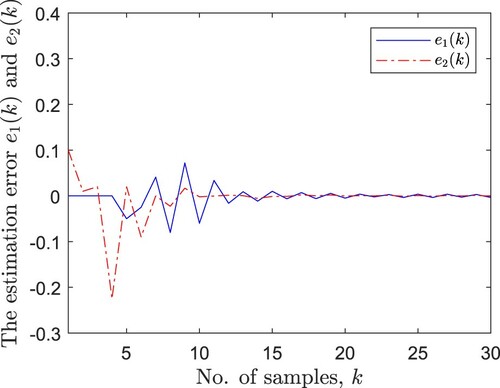Figures 2–3 are the trajectories of state vector $x\left(k\right)$ and estimation $\hat{x}\left(k\right)$. Respectively, it can be seen that the designed estimator can estimate the real neuron state effectively. Figure 4 shows the evolution of the estimate error, which indicates that the estimate error tends to zero over time.

Figure 1. The variation of the time-varying delay $\tau \left(k\right)$.

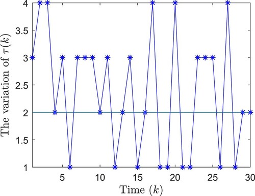
Figure 2. State $x_1\left(k\right)$ and its estimation ${\hat{x}}_1\left(k\right)$.

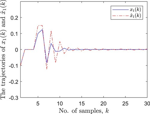
Figure 3. State $x_2\left(k\right)$ and its estimation ${\hat{x}}_2\left(k\right)$.

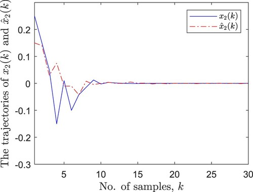
Figure 4. Estimation error of $e_1\left(k\right)$ and $e_2\left(k\right)$.

By means of the Matlab software, the desired estimator gain is outlined as follows $K=\left[\begin{array}{c}\begin{array}{cc}0.6831& 1.2983\\ 0.3966& 0.8930\end{array}\end{array}\right].$

5. Conclusion

In this paper, we have studied the problem of state estimation for a class of time delay MNNs with signal quantization. A random variable subjecting to the Bernoulli distribution has been used to represent the probabilities of the two interval values of the time-varying delay. Based on the state-dependent nature of MNNs, a signal quantization state estimation method has been designed by using Lyapunov-Krasovskii functional and stochastic analysis technique, and sufficient conditions have been provided to ensure the mean square asymptotical stability of augmented system and the specified $H_{\mathrm{\infty }}$ performance requirement. Finally, a numerical example has been provided to verify the effectiveness of the proposed estimator design method. The future research direction is to extend the results of this paper to MNNs with PTD, where the PTD is distributed in N time delay intervals with known probability.

Disclosure statement

No potential conflict of interest was reported by the authors.

References

- Bao, H., & Cao, J. (2010). Delay-distribution-dependent state estimation for discrete-time stochastic neural networks with random delay. Neural Networks, 24(1), 19–28. https://doi.org/https://doi.org/10.1016/j.neunet.2010.09.010
- Bao, H., Cao, J., & Kurths, J. (2018). State estimation of fractional-order delayed memristive neural networks. Nonlinear Dynamics, 94(2), 1215–1225. https://doi.org/https://doi.org/10.1007/s11071-018-4419-3
- Boyd, S., Ghaoui, L. E., Feron, E., & Balakrishnan, V. (1994). Linear matrix inequalities in system and control theory. SIAM.
- Chen, C., Zhu, S., Wei, Y., & Yang, C. (2020). Finite-time stability of delayed memristor-based fractional-order neural networks. IEEE Transactions on Cybernetics, 50(4), 1607–1616. https://doi.org/https://doi.org/10.1109/TCYB.6221036
- Chen, D., Chen, W., Hu, J., & Liu, H. (2019). Variance-constrained filtering for discrete-time genetic regulatory networks with state delay and random measurement delay. International Journal of Systems Science, 50(2), 231–243. https://doi.org/https://doi.org/10.1080/00207721.2018.1542045
- Chen, L., Li, C., Huang, T., & Chen, Y. (2014). Memristor crossbar-based unsupervised image learning. Neural Computing and Applications, 25(2), 393–400. https://doi.org/https://doi.org/10.1007/s00521-013-1501-0
- Chen, Y., Chen, Z., Chen, Z., & Xue, A. (2020). Observer-based passive control of non-homogeneous Markov jump systems with random communication delays. International Journal of Systems Science, 51(6), 1133–1147. https://doi.org/https://doi.org/10.1080/00207721.2020.1752844
- Ding, D., Wang, Z., & Ho, D. W. C. (2017). Distributed recursive filtering for stochastic systems under uniform quantizations and deception attacks through sensor networks. Automatica, 78(1), 231–240. https://doi.org/https://doi.org/10.1016/j.automatica.2016.12.026
- Elia, N., & Mitter, S. K. (2001). Stabilization of linear systems with limited information. IEEE Transactions on Automatic Control, 46(9), 1394–1400. https://doi.org/https://doi.org/10.1109/9.948466
- Fei, Z., & Li, S. (2018). State estimation for neural networks with random delays and stochastic communication protocol. Systems Science and Control Engineering: An Open Access Journal, 6(3), 54–63. https://doi.org/https://doi.org/10.1080/21642583.2018.1532356
- Fu, M., & Xie, L. (2005). The sector bound approach to quantized feedback control. IEEE Transactions on Automatic Control, 50(11), 1698–1711. https://doi.org/https://doi.org/10.1109/TAC.2005.858689
- Fu, Q., Cai, J., Zhong, S., & Yu, Y. (2019). Pinning impulsive synchronization of stochastic memristor-based neural networks with time-varying delays. International Journal of Control Automation and Systems, 17(1), 243–252. https://doi.org/https://doi.org/10.1007/s12555-018-0295-3
- García-Ligero, M. J., Hermoso-Carazo, A., & Linares-Pérez, J. (2020). Least-squares estimators for systems with stochastic sensor gain degradation, correlated measurement noises and delays in transmission modelled by Markov chains. International Journal of Systems Science, 51(4), 731–745. https://doi.org/https://doi.org/10.1080/00207721.2020.1737757
- Gu, Z., Zhang, J., & Du, L. (2011). Fault tolerant control for a class of time-delay syatems with intermittent actuators failure. Control and Decision, 12(26), 1829–1834. https://doi.org/https://doi.org/10.13195/j.cd.2011.12.71.guzh.016
- Hu, J., Wang, Z., Liu, G., & Zhang, H. (2020). Variance constrained recursive state estimation for time-varying complex networks with quantized measurements and uncertain inner coupling. IEEE Transactions on Neural Networks and Learning Systems, 31(6), 1955–1967. https://doi.org/https://doi.org/10.1109/TNNLS.5962385
- Hu, J., Wang, Z., & Shen, B. (2013). Quantised recursive filtering for a class of nonlinear systems with multiplicative noises and missing measurements. International Journal of Control, 86(4), 650–663. https://doi.org/https://doi.org/10.1080/00207179.2012.756149
- Hu, J., Zhang, H., Yu, X., Liu, H., & Chen, D. (2021). Design of sliding-mode-based control for nonlinear systems with mixed-delays and packet losses under uncertain missing probability. IEEE Transactions on Systems, Man, and Cybernetics: Systems, 51(5), 3217–3228. https://doi.org/https://doi.org/10.1109/TSMC.2019.2919513
- Huang, H., Huang, T., & Chen, X. (2015). Further result on guaranteed H∞ performance state estimation of delayed static neural networks. IEEE Transactions on Neural Networks and Learning Systems, 26(6), 1335–1341. https://doi.org/https://doi.org/10.1109/TNNLS.2014.2334511
- Krimi, H. R., & Gao, H. (2009). New delay-dependent exponential H∞ synchronization for uncertain neural networks with mixed time delays. IEEE Transactions on Systems, Man, and Cybernetics-Cybernetics, 40(1), 173–185. https://doi.org/https://doi.org/10.1109/TSMCB.3477
- Li, J., Wang, Z., Dong, H., & Fei, W. (2020). Delay-distribution-dependent state estimation for neural networks under stochastic communication protocol with uncertain transition probabilities. Neural Networks, 130(1), 143–151. https://doi.org/https://doi.org/10.1016/j.neunet.2020.06.023
- Li, X., Fang, J., & Li, H. (2018). Exponential synchronization of stochastic memristive recurrent neural networks under alternate state feedback control. International Journal of Control Automation and Systems, 16(6), 2859–2869. https://doi.org/https://doi.org/10.1007/s12555-018-0225-4
- Liu, H., Wang, Z., Shen, B., & Fuad, E. A. (2018). Stability analysis for discrete time stochastic memristive neural networks with both leakage and probabilistic delays. Neural Networks, 102(7), 1–9. https://doi.org/https://doi.org/10.1016/j.neunet.2018.02.003
- Lu, C., Zhang, X., Wu, M., & Yong, H. (2018). Energy-to-peak state estimation for static neural networks with interval time-varying delays. IEEE Transactions on Cybernetics, 48(10), 2823–2835. https://doi.org/https://doi.org/10.1109/TCYB.2018.2836977
- Mao, J., Ding, D., Wei, G., & Liu, H. (2019). Networked recursive filtering for time-delayed nonlinear stochastic systems with uniform quantisation under Round-Robin protocol. International Journal of Systems Science, 50(4), 871–884. https://doi.org/https://doi.org/10.1080/00207721.2019.1586002
- Petersen, I. R., & Hollot, C. V. (1986). A riccati equation approach to the stabilization of uncertain linear systems. Automatica, 22(4), 397–411. https://doi.org/https://doi.org/10.1016/0005-1098(86)90045-2
- Sakthivel, R., Anbuvithya, R., Mathiyalagan, K., & Prakash, P. (2015). Combined H∞ and passivity state estimation of memristive neural networks with random gain fluctuations. Neurocomputing, 168, 1111–1120. https://doi.org/https://doi.org/10.1016/j.neucom.2015.05.012
- Shen, B., Wang, Z., & Qiao, H. (2017). Event-triggered state estimation for discrete-time multi delayed neural networks with stochastic parameters and incomplete measurements. IEEE Transactions on Neural Networks and Learning Systems, 28(5), 1152–1163. https://doi.org/https://doi.org/10.1109/TNNLS.2016.2516030
- Song, Q., Yan, H., Zhao, Z., & Liu, Y. (2016). Global exponential stability of impulsive complex-valued neural networks with both asynchronous time-varying and continuously distributed delays. Neural Networks, 81, 1–10. https://doi.org/https://doi.org/10.1016/j.neunet.2016.04.012
- Struov, D. B., Snider, G. S., Stewart, D. R., & Williams, R. S. (2008). The missing memristor found. Nature, 453(7191), 80–83. https://doi.org/https://doi.org/10.1038/nature06932
- Wu, A., Wen, S., & Zeng, Z. (2012). Synchronization control of a class of memristor-based recurrent neural networks. Information Sciences: An International Journal, 183(1), 106–116. https://doi.org/https://doi.org/10.1016/j.ins.2011.07.044
- Yue, D., Zhang, Y., Tian, E., & Chen, T. (2008). Delay-distribution-dependent exponential stability criteria for discrete-time recurrent neural networks with stochastic delay. IEEE Transactions on Neural Networks, 19(7), 1299–1306. https://doi.org/https://doi.org/10.1109/TNN.2008.2000166
- Zhang, J., Wang, Z., Ding, D., & Liu, X. (2015). H∞ state estimation for discrete-time delayed neural networks with randomly occurring quantizations and missing measurements. Neurocomputing, 148(September (5)), 388–396. https://doi.org/https://doi.org/10.1016/j.neucom.2014.06.017
- Zhang, R., Zeng, D., & Park, J. H. (2018). Quantized sampled-data control for synchronization of inertial neural networks with heterogeneous time-varying delays. IEEE Transactions on Neural Networks and Learning Systems, 29(12), 6385–6395. https://doi.org/https://doi.org/10.1109/TNNLS.2018.2836339
- Zhang, W., Yang, S., Li, C., Zhang, W., & Yang, X. (2018). Stochastic exponential synchronization of memristive neural networks with time-varying delays via quantized control. Neural Networks, 104(1), 93–103. https://doi.org/https://doi.org/10.1016/j.neunet.2018.04.010
- Zhang, X., & Han, Q. (2018). State estimation for static neural networks with time-varying delays based on an improved reciprocally convex inequality. IEEE Transactions on Neural Networks and Learning Systems, 29(4), 1376–1381. https://doi.org/https://doi.org/10.1109/TNNLS.2017.2661862
- Zhang, X., Wu, M., & He, Y. (2003). On delay-dependent stability for linear systems with delay. Journal of Circuits and Systems, 8(3), 118–120. CNKI:SUN:DLYX.0.2003-04-001
- Zhu, S., Yang, Q., & Shen, Y. (2016). Noise further expresses exponential decay for globally exponentially stable time-varying delayed neural networks. Neural Networks, 77, 7–13. https://doi.org/https://doi.org/10.1016/j.neunet.2016.01.012