A mobile sensing approach to distributed consensus filtering of 2D stochastic nonlinear parabolic systems with disturbances

Abstract

The focus of this paper is on distributed consensus filtering in two-dimensional (2D) space for stochastic nonlinear parabolic systems with disturbances. Distributed filters are used in mobile sensor networks to achieve consensus estimate. By utilizing a mobile sensing approach, the optimal framework for parabolic systems to improve filtering performance is provided. Sufficient conditions are created under the filtering error is boundedness by employing operator-dependent Lyapunov functional. The velocity law of each mobile sensor can also be used to guide the filtering error system toward rapid convergence. Finally, numerical examples are used to verify the effectiveness of the suggested approach.

Keywords:

• Distributed filtering
• consensus performance
• mobile sensing approach
• stochastic nonlinear parabolic systems
• sector bounded disturbances
• 2D systems

1. Introduction

In the real world, most physical processes can be viewed as the evolution of parabolic systems. A number of applications employing this kind of system have started attracting growing interest, such as heat conduction, toxic gas diffusion, large-scale population movements and other processes in which evolution is a function of time and space. Observer-based control and signal processing are both fundamentally concerned with filtering parabolic systems.

As early as the early 1960s, the Kalman type filter, coupled with a weighted least squares approach (Meditch, 1971), variance method (Sakawa, 1972), and other techniques were used to analyse several filtering problems of linear parabolic systems to achieve optimal state estimation. After that, we extend the issue of filtering in parabolic systems to discrete cases, and we apply them to the study of air pollution (Omatu & Seinfeld, 1981).

Until date, the Kalman filter has remained one of the most effective methods for estimating measurement data. For networked control systems that gather information using a centralized structure, extended Kalman filtering (Hu et al., 2012), finite-horizon filtering (Wang et al., 2005) and $H_{\mathrm{\infty }}$ filtering (He et al., 2007) have all been extensively studied. Such a design of a centralized observer for one-dimensional heat conduction processes (Hidayat et al., 2011), even their fractional-order processes (Chen et al., 2020), has also yielded meaningful results.

Unfortunately, the communication between nodes in sensor networks has limitations in practical applications, owing to the limitations of energy, bandwidth and range. Data fusion can be carried out in a distributed way, which means that each node can only communicate with its neighbours. For distributed strategies, switched system approach (Zhang et al., 2016), event-triggered mechanism (Li et al., 2020), fuzzy system method (Zhang et al., 2017) and Round-Robin type protocol (Ugrinovskii & Fridman, 2014) have been raised to study the distributed filtering issue for networked control systems.

Distributed estimation has now been the major tool for investigating filtering challenges involving stochastic parameters and nonlinearities in sensor networks with incomplete data. Sensor networks with incomplete data were used to investigate distributed filtering challenges for stochastic systems (Ding et al., 2012; Yu et al., 2013). In addition, Liu et al. (2015) addressed a recursive distributed filter using an event-triggered mechanism in which each sensor node communicates intermittently across sensor networks.

The consensus performance criterion was employed as a significant index to express the bounded consensus in terms of filtering error in Shen, Wang, and Hung  (2010) and Yu et al. (2009). Distributed estimation is effective for consensus. Distributed consensus estimation combined with receding horizon techniques (Xu et al., 2022) has also been deeply investigated in distributed parameter systems.

Parabolic systems can be affected by noise for realistic physical processes. The disturbances might appear probabilistically. A randomly occurring nonlinearities (RONs) model is used to represent the nonlinear terms, which occur randomly, in the system. Numerous studies (Duan et al., 2014; Liu et al., 2011; Shen et al., 2011) on RONs have been suggested.

A networked environment is where data missing phenomena often arises due to sensor temporal failure or network transmission delays. In Nahi (1969), a method to deal with the data missing by using a Bernoulli distribution has been first presented and then investigated in Wei et al. (2009) and Shen, Wang, and Hung  (2010) for the various filtering issues of networked control systems with probabilistic packet losses. Furthermore, signal quantization frequently occurs prior to transmission in a networked setting due to the constrained network bandwidth. It was noted that logarithmic quantization is suitable for communication with fewer bits. The sector bound technique has been extensively adopted for the quantization effects in Shen, Wang, Shu, et al. (2010).

As mentioned previously, most of the current filtering issues for systems adopt static sensor networks. Mobile sensor networks are receiving a lot of attention in the engineering industry since for their advantages of flexibility and energy reduction. For stochastic nonlinear parabolic systems using mobile sensor networks, the distributed consensus filtering challenge has not been well studied and is yet open.

The filtering issue for stochastic nonlinear parabolic systems with disturbances will be the subject of this study. Distributed consensus filters are constructed in two-dimensional (2D) space with the aid of mobile sensors. In this study, mobile sensing as a novel method will yield some innovative findings for the filtering issue of 2D parabolic systems.

2. Problem formulation and preliminaries

Consider a stochastic nonlinear parabolic system that describes a target process on a 2D plane. (1) $\begin{array}{rl}\frac{\mathrm{\partial }Q(t,\theta )}{\mathrm{\partial }t}& =\sum _{k=1}^2\frac{\mathrm{\partial }}{\mathrm{\partial }{\theta }_k}\left(a_k\right({\theta }_k\left)\frac{\mathrm{\partial }Q(t,\theta )}{\mathrm{\partial }{\theta }_k}\right)\\ & +\gamma \left(t\right)Cf(t,Q(t,\theta \left)\right)+\sigma \left(t\right)\frac{\mathrm{d}\omega }{\mathrm{d}t},\end{array}$(1) where $Q(t,\theta )$ denotes the state of the 2D parabolic system at moment $t\in {\mathbf{\text{R}}}^{+}$, located at plane $\theta =({\theta }_1,{\theta }_2)$. The diffusion coefficients $a_k\left({\xi }_k\right)\ge a_0>0,k=1,2$. $\sigma \left(t\right)$ is an external disturbance noise, and $\sigma \left(t\right)$ is a 2D Brownian motion with $\mathbb{E}\left\{\mathrm{d}\omega \right(t\left)\right\}=0$ and variance $\mathbb{D}\left\{\mathrm{d}\omega \right(t\left)\right\}=1$. C denotes the strength coefficient of $f(t,Q(t,\theta \left)\right)$. Stochastic variable $\gamma \left(t\right)\in \mathbf{\text{R}}$ is a Bernoulli distributed white sequence taking values of 1 and 0 with (2) $\begin{array}{r}\{\begin{array}{l}\mathrm{P}\mathrm{r}\mathrm{o}\mathrm{b}\left\{\gamma \right(t)=1\}=\overline{\gamma },\\ \mathrm{P}\mathrm{r}\mathrm{o}\mathrm{b}\left\{\gamma \right(t)=0\}=1-\overline{\gamma },\end{array}\end{array}$(2) where $\overline{\gamma }\in [0,1]$ are known positive constants. It is assumed that the stochastic variables $\gamma \left(t\right)$ is independent of both $\sigma \left(t\right)$ and the initial state of system. Hence, we have $\mathbb{E}\left\{\gamma \right(t\left)\right\}=\overline{\gamma }$.

Outputs from N mobile sensors measured spatially. In this case, ith mobile sensor can provide output as follows: (3) $\begin{array}{rl}{y}_i\left(t\right)& ={\alpha }_i\left(t\right){\iint }_S{\phi }_i(\theta ;{\theta }_i(t\left)\right)Q(t,\theta )\mathrm{d}S+d_i\left(t\right)\frac{\mathrm{d}{\nu }_i}{\mathrm{d}t},\\ & i=1,2,\dots ,N,\end{array}$(3) where $d_i\left(t\right)$ is external noise of ith mobile sensor, and ${\nu }_i\left(t\right)$ is an independent 2D Brownian motion with $\mathbb{E}\left\{\mathrm{d}{\nu }_i\right(t\left)\right\}=0$ and variance $\mathbb{D}\left\{\mathrm{d}{\nu }_i\right(t\left)\right\}=1,i=1,2,\dots ,N$.

${\phi }_i(\theta ;{\theta }_i(t\left)\right)={\phi }_i({\theta }_1,{\theta }_2;{\theta }_{i1}(t),{\theta }_{i2}(t\left)\right)$ refers to the spatial distribution of ith sensing device. It is usually assumed that distribution function ${\phi }_i(\theta ;{\theta }_i(t\left)\right)$ is non-negative and bounded and is expressed by (4) $\begin{array}{r}{\phi }_i({\theta }_j;{\theta }_{ij}(t\left)\right)=\{\begin{array}{ll}{\displaystyle \frac{1}{{\chi }_{ij}}}& \mathrm{i}\mathrm{f}{\theta }_j\in [{\theta }_{ij}-{ϵ}_{ij},{\theta }_{ij}+{ϵ}_{ij}],j=1,2,\\ 0& \mathrm{o}\mathrm{t}\mathrm{h}\mathrm{e}\mathrm{r}\mathrm{w}\mathrm{i}\mathrm{s}\mathrm{e},\end{array}\end{array}$(4) where ${\theta }_1\in S_{i1}=[{\theta }_{i1}-{ϵ}_{i1},{\theta }_{i1}+{ϵ}_{i1}]$, ${\theta }_2\in S_{i2}=[{\theta }_{i2}-{ϵ}_{i2},{\theta }_{i2}+{ϵ}_{i2}]$ and $S_i=S_{i1}\times S_{i2}$.

The distribution function shows that the distribution of each mobile sensor may also be different. Each moving sensing device is located at $\left({\theta }_{i1}\right(t),{\theta }_{i2}(t\left)\right)$. The time-varying location function changes with time, which characterizes the spatiotemporal trajectory of each mobile sensor. For every i, the stochastic variable ${\alpha }_i\left(t\right)\in \mathbf{\text{R}},i=1,2,\dots ,N$ is a Bernoulli distributed white sequence taking values of 1 and 0 with (5) $\begin{array}{r}\{\begin{array}{l}\mathrm{P}\mathrm{r}\mathrm{o}\mathrm{b}\left\{{\alpha }_i\right(t)=1\}={\overline{\alpha }}_i,\\ \mathrm{P}\mathrm{r}\mathrm{o}\mathrm{b}\left\{{\alpha }_i\right(t)=0\}=1-{\overline{\alpha }}_i,\end{array}\end{array}$(5) where ${\overline{\alpha }}_i\in [0,1],i=1,2,\dots ,N$ are known positive constants. It is assumed that the stochastic variables ${\alpha }_i\left(t\right)$ is independent of both $d_i\left(t\right)$ and the initial state of system. Accordingly, we have (6) $\begin{array}{r}\mathbb{E}\left\{{\alpha }_i\right(t)-{\overline{\alpha }}_i\}=0\mathrm{a}\mathrm{n}\mathrm{d}\mathbb{E}\left\{\right({\alpha }_i\left(t\right)-{\overline{\alpha }}_i{)}^2\}={\overline{\alpha }}_i(1-{\overline{\alpha }}_i).\end{array}$(6) In addition, the quantization effects are taken into account in this study. The quantizer $q(\cdot )$ is defined as $\overline{y}\left(t\right)=q\left(y\right(t\left)\right)=\left[q_1\right(y_1\left(t\right)),q_2(y_2\left(t\right)),\dots ,q_N(y_N\left(t\right)){]}^T.$$\overline{y}\left(t\right)\in {\mathrm{R}}^N$ is the signals which have been quantized. $\overline{y}\left(t\right)$ would then be sent via the filter. The set of quantization levels for each $q_i(\cdot )$ is provided by $\begin{array}{rl}& {\mathcal{U}}_i=\{\pm u_{\iota }^{\left(i\right)},u_{\iota }^{\left(i\right)}={\rho }_{\iota }^{\left(i\right)}{u}_0^{\left(i\right)},\iota =0,\pm 1,\pm 2,\dots \}\cup \left\{0\right\},\\ & 0\le {\rho }_{\iota }\le 1,u_0^{\left(i\right)}>0,\end{array}$where ${\rho }^{\left(i\right)}$ represents the quantization density and is a constant. The logarithmic type quantizer $q(\cdot )$ is provided by $q_i\left(y_i\right(t\left)\right)=\{\begin{array}{ll}{\chi }_{\iota }^{\left(i\right)},& {\displaystyle \frac{1}{1+{\delta }_i}{\chi }_{\iota }^{\left(i\right)}<y_i\left(t\right)}\\ & \le \frac{1}{1-{\delta }_i}{\chi }_{\iota }^{\left(i\right)},\\ 0,& y_i\left(t\right)=0,\\ -q(-y_i(t\left)\right),& y_i\left(t\right)<0,\end{array}$where ${\delta }_i=(1-{\rho }_i)/(1+{\rho }_i)$. As a result of Shen, Wang, Shu, et al. (2010), for certain ${\mathrm{\Delta }}_i\left(t\right)$ satisfying $|{\mathrm{\Delta }}_i\left(t\right)|\le {\delta }_i$, can be stated as $q\left(y_i\right(t\left)\right)=(1+{\mathrm{\Delta }}_i(t\left)\right)y_i\left(t\right)$.

After quantization, the measurements can be expressed as (7) $\begin{array}{r}{\overline{y}}_i\left(t\right)=(1+{\mathrm{\Delta }}_i(t\left)\right)y_i\left(t\right).\end{array}$(7) As a way of rewriting the 2D parabolic system (1(1) $\begin{array}{rl}\frac{\mathrm{\partial }Q(t,\theta )}{\mathrm{\partial }t}& =\sum _{k=1}^2\frac{\mathrm{\partial }}{\mathrm{\partial }{\theta }_k}\left(a_k\right({\theta }_k\left)\frac{\mathrm{\partial }Q(t,\theta )}{\mathrm{\partial }{\theta }_k}\right)\\ & +\gamma \left(t\right)Cf(t,Q(t,\theta \left)\right)+\sigma \left(t\right)\frac{\mathrm{d}\omega }{\mathrm{d}t},\end{array}$(1) ) in the abstract form, a few symbols and their meanings are given here.

Let $\mathcal{H}$ be a Hilbert space. The inner product of $\mathcal{H}$ is $〈\cdot ,\cdot 〉$ and its induced norm is $|\cdot |$. Let $\mathcal{B}$ be a reflexive Banach space. $\Vert \cdot \Vert$ denotes the norm of $\mathcal{B}$. It is assumed that $\mathcal{B}$ occupies embedded densely and continuously in $\mathcal{H}$. Let ${\mathcal{B}}^{\ast }$ denotes the conjugate dual of $\mathcal{B}$. Notice that we have $|\phi |\le b\Vert \phi \Vert ,\phi \in \mathcal{B}$, for any positive constant $b$.

The abstract form of the 2D parabolic system is then as follows: (8) $\begin{array}{r}\mathrm{d}Q\left(t\right)=\left(\mathcal{A}Q\right(t)+\gamma (t\left)CF\right(t,Q\left(t\right)\left)\right)\mathrm{d}t+\sigma \left(t\right)\mathrm{d}\omega ,\end{array}$(8) where the state of system $Q(t,\cdot )=\left\{Q\right(t,\theta ):0\le {\theta }_j\le l_j,j=1,2\}$ is in space $\mathcal{H}=L_2\left(S\right)$. The Sobolev space $\mathcal{B}=H_0^1(0,l)=\{\psi \in H^1(\mathrm{\Omega }\left)|\psi \right(0)=\psi (l)=0\}$ and its conjugate dual space is $H^{-1}\left(S\right)$. Let infinitesimal operator $\mathcal{A}=\frac{\mathrm{d}}{\mathrm{d}{\theta }_1}\left(a\right({\theta }_1\left)\frac{\mathrm{d}}{\mathrm{d}{\theta }_1}\right)+\frac{\mathrm{d}}{\mathrm{d}{\theta }_2}\left(a\right({\theta }_2\left)\frac{\mathrm{d}}{\mathrm{d}{\theta }_2}\right)$ and its domain is given by $\mathcal{D}\left(\mathcal{A}\right)=\{\psi \in L_2(S):\psi ,{\psi }^{\prime }\mathrm{a}\mathrm{r}\mathrm{e}\mathrm{a}\mathrm{b}\mathrm{s}\mathrm{o}\mathrm{l}\mathrm{u}\mathrm{t}\mathrm{e}\mathrm{l}\mathrm{y}\mathrm{c}\mathrm{o}\mathrm{n}\mathrm{t}\mathrm{i}\mathrm{n}\mathrm{u}\mathrm{o}\mathrm{u}\mathrm{s},{\psi }^{″}\in L_2(S\left)\mathrm{a}\mathrm{n}\mathrm{d}\psi \right(0)=\psi (l_j)=0,j=1,2\}$. The linear bounded operator $\mathcal{A}$ satisfying $|〈f,\mathcal{A}g〉|\le {\alpha }_0\Vert f\Vert \Vert g\Vert$, for $f,g\in \mathcal{B}$ and constant ${\alpha }_0>0$. $-\mathcal{A}>0$ is coercive, i.e. $〈g,-\mathcal{A}g〉\ge {\text{β}}_0\Vert g{\Vert }^2$, for $g\in \mathcal{B}$ and constant ${\text{β}}_0>0$.

The measurement output can be expressed by (9) $\begin{array}{rl}{\overline{y}}_i\left(t\right)& =(1+{\mathrm{\Delta }}_i(t\left)\right){\alpha }_i\left(t\right){\Phi }_i\left({\theta }_i\right(t\left)\right)Q\left(t\right)\\ & +d_i\left(t\right)\frac{\mathrm{d}{\nu }_i}{\mathrm{d}t},i=1,2,\dots ,N.\end{array}$(9) The nonlinear function f satisfies the following Assumption 2.1.

Assumption 2.1

There exists a constant l such that (10) $\begin{array}{r}(s_1-s_2{)}^T(F(t,s_1(t\left)\right)-F(t,s_2(t\left)\right))\le l(s_1-s_2{)}^T(s_1-s_2)\end{array}$(10) holds, for all $s_1,s_2\in L_2\left(S\right)$.

Assumption 2.2

Disturbances $\sigma \left(t\right)$ and $d_i\left(t\right)$ are sector bounded and satisfying (11) $\begin{array}{rl}{\sigma }^T\left(t\right)\sigma \left(t\right)& \le \vartheta ,\end{array}$(11) (12) $\begin{array}{rl}{d}_i^T\left(t\right)d_i\left(t\right)& \le {\eta }_i,\end{array}$(12) where $\vartheta >0$ and ${\eta }_i>0,i=1,2,\dots ,N$ are constants.

Assumption 2.3

Linear operator $\Phi \left(\theta \right(t\left)\right)$ is bounded, that is $〈g,\Phi \left(\theta \right(t\left)\right)g〉\le {\mu }_c〈g,g〉.$It is to be noted that the observation operator is self-adjoint due to the symmetry of the spatial distribution ${\phi }_i(\theta ;{\theta }_i(t\left)\right)$, and its norm is determined by the embedding constant b and the measure of the spatial domain $L\left(S\right)$.

Definition 2.1 is presented in the following to get the main results.

Definition 2.1

Distributed consensus performance

The filters are said to be distributed consensus filters if there exist ${\eta }_i>0$ and $\mu >0$ such that (13) $\begin{array}{r}\underset{t\to \mathrm{\infty }}{lim}\frac{1}{N}\mathbb{E}\left(\sum _{i=1}^N|{\hat{Q}}_i\right(t)-Q(t\left){|}^2\right)\le \sum _{i=1}^N{\sigma }_i{\eta }_i+\mu \vartheta .\end{array}$(13)

3. Main results and proofs

The distributed consensus filter is designed for the ith mobile sensor in this paper: (14) $\begin{array}{rl}{\dot{\hat{Q}}}_i\left(t\right)& =\mathcal{A}{\hat{Q}}_i\left(t\right)+\overline{\gamma }CF(t,{\hat{Q}}_i(t\left)\right)+{\Phi }_i^{\ast }\left({\theta }_i\right(t\left)\right)k_i\\ & \times \left({\overline{y}}_i\right(t)-(1+{\delta }_i\left){\overline{\alpha }}_i{\Phi }_i\right({\theta }_i\left(t\right)\left){\hat{Q}}_i\right(t\left)\right)\\ & +G_i\kappa \sum _{j=1}^N{b}_{ij}{\hat{Q}}_j\left(t\right),\end{array}$(14) where ${\hat{Q}}_i\left(t\right)$ is the ith mobile sensor's state estimation. ${\overline{y}}_i\left(t\right),i=1,2,\dots ,N$ is output measurement of the ith mobile sensor. As the adjoint of ${\Phi }^{\ast }\left(\theta \right(t\left)\right)$, $\Phi \left(\theta \right(t\left)\right)$ performs the observation operator. $k_i>0,i=1,2,\dots ,N$ is the observer gain and $G_i,i=1,2,\dots ,N$ is the consensus filter gain. In addition, ${\hat{Q}}_i\left(0\right)={\hat{Q}}_{i0}\ne Q\left(0\right)$ for all $i=1,2,\dots ,N$. $B=(b_{ij}{)}_{N\times N}$ is irreducible, $b_{ij}=b_{ji}\ge 0$, for $i\ne j$ and $\sum _{j=1}^N{b}_{ij}=0$, for all $i=1,2,\dots ,N$. It is obvious that B has an eigenvalue of zero, and all other eigenvalues are negative.

Letting $e_i\left(t\right)={\hat{Q}}_i\left(t\right)-Q\left(t\right)$, the filtering error dynamical system can be expressed as follows: (15) $\begin{array}{rl}\mathrm{d}{e}_i\left(t\right)& ={\mathcal{A}}_{\varphi }\left({\theta }_i\right(t\left)\right)e_i\left(t\right)+\overline{\gamma }CF(t,e_i(t\left)\right)\\ & +(\overline{\gamma }-\gamma (t\left)\right)CF(t,Q(t,\theta \left)\right)\\ & -k_i{\Phi }_i^{\ast }\left({\theta }_i\right(t\left)\right)\left[\right(1+{\delta }_i){\overline{\alpha }}_i\\ & -(1+{\mathrm{\Delta }}_i(t\left)\right){\alpha }_i\left(t\right)\left]{\Phi }_i\right({\theta }_i\left(t\right)\left)Q\right(t)\\ & +G_i\kappa \sum _{j=1}^N{b}_{ij}{e}_j\left(t\right)-\sigma \left(t\right)\mathrm{d}\omega \\ & +{\Phi }_i^{\ast }\left({\theta }_i\right(t\left)\right)k_i{d}_i\left(t\right)\mathrm{d}{\nu }_i,\end{array}$(15) where ${\mathcal{A}}_{\varphi }\left({\theta }_i\right(t\left)\right)=\mathcal{A}-k_i(1+{\delta }_i){\overline{\alpha }}_i{\Phi }_i^{\ast }\left({\theta }_i\right(t\left)\right){\Phi }_i\left({\theta }_i\right(t\left)\right)$ and $F(t,e_i(t\left)\right)=F(t,{\hat{Q}}_i(t\left)\right)-F(t,Q(t\left)\right)$.

Given that $\Phi \left({\theta }_i\right(t\left)\right)$ is self-adjoint, it follows that the closed-loop operator ${\mathcal{A}}_{\varphi }\left({\theta }_i\right(t\left)\right)$ is also self-adjoint. Moreover, it can be known that the ${\mathcal{A}}_{\varphi }\left({\theta }_i\right(t\left)\right)$ is invertible when the boundedness and coercivity of $\mathcal{A}$ and Assumption 2.3 are considered combined.

3.1. Bounded consensus analysis

Theorem 3.1

Under Assumptions 2.1–2.3, the filters (14(14) $\begin{array}{rl}{\dot{\hat{Q}}}_i\left(t\right)& =\mathcal{A}{\hat{Q}}_i\left(t\right)+\overline{\gamma }CF(t,{\hat{Q}}_i(t\left)\right)+{\Phi }_i^{\ast }\left({\theta }_i\right(t\left)\right)k_i\\ & \times \left({\overline{y}}_i\right(t)-(1+{\delta }_i\left){\overline{\alpha }}_i{\Phi }_i\right({\theta }_i\left(t\right)\left){\hat{Q}}_i\right(t\left)\right)\\ & +G_i\kappa \sum _{j=1}^N{b}_{ij}{\hat{Q}}_j\left(t\right),\end{array}$(14) ) are distributed consensus filters if (16) $\begin{array}{r}\overline{\gamma }l+\kappa {\lambda }_{max}\left(B\right)<0,\end{array}$(16) and the velocity law of ith mobile sensor as follows: (17) $\begin{array}{rl}{\dot{\theta }}_{i1}\left(t\right)& =-{\rho }_{i1}{k}_i(1+{\delta }_i){\overline{\alpha }}_i{\mathrm{\Omega }}_{i1},\end{array}$(17) (18) $\begin{array}{rl}{\dot{\theta }}_{i2}\left(t\right)& =-{\rho }_{i2}{k}_i(1+{\delta }_i){\overline{\alpha }}_i{\mathrm{\Omega }}_{i2},\end{array}$(18) where ${\mathrm{\Omega }}_{i1}=e_i^2(t,{\theta }_{i1}-{ϵ}_{i1})-e_i^2(t,{\theta }_{i1}+{ϵ}_{i1}),{\mathrm{\Omega }}_{i2}=e_i^2(t,{\theta }_{i2}-{ϵ}_{i2})-e_i^2(t,{\theta }_{i2}+{ϵ}_{i2})$ with ${\rho }_{i1}>0,{\rho }_{i2}>0$ arevelocity gain of each mobile sensor. The estimated bound is presented as follows: (19) $\begin{array}{r}\underset{t\to \mathrm{\infty }}{lim}\frac{1}{N}\mathbb{E}\left(\sum _{i=1}^N|{\hat{Q}}_i\right(t)-Q(t\left){|}^2\right)\le \frac{\vartheta +\frac{{\mu }_c^2}{N}\sum _{i=1}^N{k}_i^2{\eta }_i}{-2(\overline{\gamma }l+\kappa {\lambda }_{max}(B\left)\right)}.\end{array}$(19)

Proof.

Taking account into the properties of the linear operator $\mathcal{A}$, the closed-loop operator ${\mathcal{A}}_{\varphi }\left({\theta }_i\right(t\left)\right)$ is easy to verify that it satisfies $|\sum _{i=1}^N〈f,{\mathcal{A}}_{\varphi }\left({\theta }_i\right(t\left)\right)g〉|\le \alpha \Vert f\Vert \Vert g\Vert$ and $\sum _{i=1}^N〈g,-{\mathcal{A}}_{\varphi }\left({\theta }_i\right(t\left)\right)g〉>{\text{β}}_{0}N\Vert g{\Vert }^2$, where $f,g\in \mathcal{B}$ and constant $\alpha >0,{\text{β}}_0>0$.

Consider the following Lyapunov functional, which is operator dependent: (20) $\begin{array}{r}V\left(t\right)=-\frac{1}{2}\sum _{i=1}^N〈e_i\left(t\right),{\mathcal{A}}_{\varphi }\left({\theta }_i\right(t\left)\right)e_i\left(t\right)〉.\end{array}$(20) In the It$\hat{\mathrm{o}}$ formula, a stochastic differentiation of (20(20) $\begin{array}{r}V\left(t\right)=-\frac{1}{2}\sum _{i=1}^N〈e_i\left(t\right),{\mathcal{A}}_{\varphi }\left({\theta }_i\right(t\left)\right)e_i\left(t\right)〉.\end{array}$(20) ) results in (21) $\begin{array}{rl}\mathrm{d}V\left(t\right)& =\mathcal{L}V\left(t\right)-\sum _{i=1}^N〈e_i\left(t\right),{\mathcal{A}}_{\varphi }\left({\theta }_i\right(t\left)\right)w\left(t\right)\mathrm{d}\omega 〉\\ & +\sum _{i=1}^N〈e_i\left(t\right),{\mathcal{A}}_{\varphi }\left({\theta }_i\right(t\left)\right){\Phi }^{\ast }\left({\theta }_i\right(t\left)\right)k_i{d}_i\left(t\right)\mathrm{d}{\nu }_i〉.\end{array}$(21) A weak infinitesimal operator defined as $\mathcal{L}V\left(t\right)=\underset{\mathrm{\Delta }\to 0^{+}}{lim}\frac{\mathbb{E}\left\{V\right(t+\mathrm{\Delta }\left)|t\right\}-V\left(t\right)}{\mathrm{\Delta }}$ along stochastic diffusion processes, according to filtering error system (15(15) $\begin{array}{rl}\mathrm{d}{e}_i\left(t\right)& ={\mathcal{A}}_{\varphi }\left({\theta }_i\right(t\left)\right)e_i\left(t\right)+\overline{\gamma }CF(t,e_i(t\left)\right)\\ & +(\overline{\gamma }-\gamma (t\left)\right)CF(t,Q(t,\theta \left)\right)\\ & -k_i{\Phi }_i^{\ast }\left({\theta }_i\right(t\left)\right)\left[\right(1+{\delta }_i){\overline{\alpha }}_i\\ & -(1+{\mathrm{\Delta }}_i(t\left)\right){\alpha }_i\left(t\right)\left]{\Phi }_i\right({\theta }_i\left(t\right)\left)Q\right(t)\\ & +G_i\kappa \sum _{j=1}^N{b}_{ij}{e}_j\left(t\right)-\sigma \left(t\right)\mathrm{d}\omega \\ & +{\Phi }_i^{\ast }\left({\theta }_i\right(t\left)\right)k_i{d}_i\left(t\right)\mathrm{d}{\nu }_i,\end{array}$(15) ), yields (22) $\begin{array}{rl}\mathcal{L}V\left(t\right)& =-\sum _{i=1}^N\mathbb{E}〈e_i\left(t\right),{\mathcal{A}}_{\varphi }\left({\theta }_i\right(t\left)\right){\dot{e}}_i\left(t\right)〉\\ & -\frac{1}{2}\sum _{i=1}^N\mathbb{E}〈e_i\left(t\right),\frac{\mathrm{d}{\mathcal{A}}_{\varphi }\left({\theta }_i\right(t\left)\right)}{\mathrm{d}t}{e}_i\left(t\right)〉\\ & +\frac{1}{2}\sum _{i=1}^N\left({\sigma }^T\right(t\left)\sigma \right(t)+k_i^2{\Phi }^{\ast }({\theta }_i\left(t\right))\\ & \times \Phi \left({\theta }_i\right(t\left)\right)d_i^T\left(t\right)d_i\left(t\right)).\end{array}$(22) In (22(22) $\begin{array}{rl}\mathcal{L}V\left(t\right)& =-\sum _{i=1}^N\mathbb{E}〈e_i\left(t\right),{\mathcal{A}}_{\varphi }\left({\theta }_i\right(t\left)\right){\dot{e}}_i\left(t\right)〉\\ & -\frac{1}{2}\sum _{i=1}^N\mathbb{E}〈e_i\left(t\right),\frac{\mathrm{d}{\mathcal{A}}_{\varphi }\left({\theta }_i\right(t\left)\right)}{\mathrm{d}t}{e}_i\left(t\right)〉\\ & +\frac{1}{2}\sum _{i=1}^N\left({\sigma }^T\right(t\left)\sigma \right(t)+k_i^2{\Phi }^{\ast }({\theta }_i\left(t\right))\\ & \times \Phi \left({\theta }_i\right(t\left)\right)d_i^T\left(t\right)d_i\left(t\right)).\end{array}$(22) ), a first term is deduced as follows: (23) $\begin{array}{rl}& -\sum _{i=1}^N\mathbb{E}〈e_i\left(t\right),{\mathcal{A}}_{\varphi }\left({\theta }_i\right(t\left)\right){\dot{e}}_i\left(t\right)〉\\ & \le -\sum _{i=1}^N\mathbb{E}〈e_i\left(t\right),{\mathcal{A}}_{\varphi }\left({\theta }_i\right(t\left)\right)\left({\mathcal{A}}_{\varphi }\right({\theta }_i\left(t\right)\left)e_i\right(t)\phantom{\sum _{j=1}^N{b}_{ij}}\\ & +\overline{\gamma }CF(t,e_i(t\left)\right)\phantom{\sum _{j=1}^N{b}_{ij}{e}_j\left(t\right)}+k_i{\Phi }_i^{\ast }\left({\theta }_i\right(t\left)\right)\\ & \times (1+{\delta }_i)\left({\alpha }_i\right(t)-{\overline{\alpha }}_i){\Phi }_i\left({\theta }_i\right(t\left)\right)Q\left(t\right)\\ & +G_i\kappa \sum _{j=1}^N{b}_{ij}{e}_j\left(t\right))〉\\ & \le -\sum _{i=1}^N|{\mathcal{A}}_{\varphi }\left({\theta }_i\right(t\left)\right)e_i\left(t\right){|}^2\\ & +\overline{\gamma }l\sum _{i=1}^N〈e_i\left(t\right),e_i\left(t\right)〉+\kappa \sum _{i=1}^N\sum _{j=1}^N{b}_{ij}〈e_i\left(t\right),e_j\left(t\right))〉\\ & \le (\overline{\gamma }l+\kappa {\lambda }_{max}(B\left)\right)\sum _{i=1}^N〈e_i\left(t\right),e_i\left(t\right)〉,\end{array}$(23) where $C=G_i=-{\mathcal{A}}_{\varphi }^{-1}\left({\theta }_i\right(t\left)\right).$

By calculating the second term in (22(22) $\begin{array}{rl}\mathcal{L}V\left(t\right)& =-\sum _{i=1}^N\mathbb{E}〈e_i\left(t\right),{\mathcal{A}}_{\varphi }\left({\theta }_i\right(t\left)\right){\dot{e}}_i\left(t\right)〉\\ & -\frac{1}{2}\sum _{i=1}^N\mathbb{E}〈e_i\left(t\right),\frac{\mathrm{d}{\mathcal{A}}_{\varphi }\left({\theta }_i\right(t\left)\right)}{\mathrm{d}t}{e}_i\left(t\right)〉\\ & +\frac{1}{2}\sum _{i=1}^N\left({\sigma }^T\right(t\left)\sigma \right(t)+k_i^2{\Phi }^{\ast }({\theta }_i\left(t\right))\\ & \times \Phi \left({\theta }_i\right(t\left)\right)d_i^T\left(t\right)d_i\left(t\right)).\end{array}$(22) ), we obtain (24) $\begin{array}{rl}& -\frac{1}{2}\sum _{i=1}^N〈e_i\left(t\right),\frac{\mathrm{d}{\mathcal{A}}_{\varphi }\left({\theta }_i\right(t\left)\right)}{\mathrm{d}t}{e}_i\left(t\right)〉\\ & =\frac{1}{2}\sum _{i=1}^N〈e_i\left(t\right),\frac{\mathrm{d}}{\mathrm{d}t}\left(k_i\right(1+{\delta }_i\left){\overline{\alpha }}_i{\Phi }_i^{\ast }\right({\theta }_i\left(t\right))\\ & \times {\Phi }_i\left({\theta }_i\right(t\left)\right)\left)e_i\right(t)〉\\ & =\sum _{i=1}^N{\dot{\theta }}_i\left(t\right)k_i(1+{\delta }_i){\overline{\alpha }}_i{\iint }_S\phi (\theta ;{\theta }_i(t\left)\right)\\ & \times \frac{\mathrm{\partial }\phi (\theta ;{\theta }_i(t\left)\right)}{\mathrm{\partial }\theta }{e}_i^2(t,\xi )\mathrm{d}S\\ & =\sum _{j=1}^2\sum _{i=1}^N{\dot{\theta }}_{ij}\left(t\right)k_i(1+{\delta }_i){\overline{\alpha }}_i{\mathrm{\Omega }}_{ij},\end{array}$(24) where ${\mathrm{\Omega }}_{ij}$ are defined in Theorem 3.1.

The choice (25) $\begin{array}{r}{\dot{\theta }}_{ij}\left(t\right)=-{\rho }_{ij}{k}_i(1+{\delta }_i){\overline{\alpha }}_i{\mathrm{\Omega }}_{ij},j=1,2,\end{array}$(25) deduces (24(24) $\begin{array}{rl}& -\frac{1}{2}\sum _{i=1}^N〈e_i\left(t\right),\frac{\mathrm{d}{\mathcal{A}}_{\varphi }\left({\theta }_i\right(t\left)\right)}{\mathrm{d}t}{e}_i\left(t\right)〉\\ & =\frac{1}{2}\sum _{i=1}^N〈e_i\left(t\right),\frac{\mathrm{d}}{\mathrm{d}t}\left(k_i\right(1+{\delta }_i\left){\overline{\alpha }}_i{\Phi }_i^{\ast }\right({\theta }_i\left(t\right))\\ & \times {\Phi }_i\left({\theta }_i\right(t\left)\right)\left)e_i\right(t)〉\\ & =\sum _{i=1}^N{\dot{\theta }}_i\left(t\right)k_i(1+{\delta }_i){\overline{\alpha }}_i{\iint }_S\phi (\theta ;{\theta }_i(t\left)\right)\\ & \times \frac{\mathrm{\partial }\phi (\theta ;{\theta }_i(t\left)\right)}{\mathrm{\partial }\theta }{e}_i^2(t,\xi )\mathrm{d}S\\ & =\sum _{j=1}^2\sum _{i=1}^N{\dot{\theta }}_{ij}\left(t\right)k_i(1+{\delta }_i){\overline{\alpha }}_i{\mathrm{\Omega }}_{ij},\end{array}$(24) ) negative definite and ${\rho }_{ij}>0$.

The last term of (22(22) $\begin{array}{rl}\mathcal{L}V\left(t\right)& =-\sum _{i=1}^N\mathbb{E}〈e_i\left(t\right),{\mathcal{A}}_{\varphi }\left({\theta }_i\right(t\left)\right){\dot{e}}_i\left(t\right)〉\\ & -\frac{1}{2}\sum _{i=1}^N\mathbb{E}〈e_i\left(t\right),\frac{\mathrm{d}{\mathcal{A}}_{\varphi }\left({\theta }_i\right(t\left)\right)}{\mathrm{d}t}{e}_i\left(t\right)〉\\ & +\frac{1}{2}\sum _{i=1}^N\left({\sigma }^T\right(t\left)\sigma \right(t)+k_i^2{\Phi }^{\ast }({\theta }_i\left(t\right))\\ & \times \Phi \left({\theta }_i\right(t\left)\right)d_i^T\left(t\right)d_i\left(t\right)).\end{array}$(22) ) gives the following: (26) $\begin{array}{rl}& \frac{1}{2}\sum _{i=1}^N\left({\sigma }^T\right(t\left)\sigma \right(t)++k_i^2{\Phi }^{\ast }({\theta }_i\left(t\right)\left)\Phi \right({\theta }_i\left(t\right)\left)d_i^T\right(t\left)d_i\right(t\left)\right)\\ & \le \frac{1}{2}N\vartheta +\frac{{\mu }_c^2}{2}\sum _{i=1}^N{k}_i^2{\eta }_i.\end{array}$(26) After combining (23(23) $\begin{array}{rl}& -\sum _{i=1}^N\mathbb{E}〈e_i\left(t\right),{\mathcal{A}}_{\varphi }\left({\theta }_i\right(t\left)\right){\dot{e}}_i\left(t\right)〉\\ & \le -\sum _{i=1}^N\mathbb{E}〈e_i\left(t\right),{\mathcal{A}}_{\varphi }\left({\theta }_i\right(t\left)\right)\left({\mathcal{A}}_{\varphi }\right({\theta }_i\left(t\right)\left)e_i\right(t)\phantom{\sum _{j=1}^N{b}_{ij}}\\ & +\overline{\gamma }CF(t,e_i(t\left)\right)\phantom{\sum _{j=1}^N{b}_{ij}{e}_j\left(t\right)}+k_i{\Phi }_i^{\ast }\left({\theta }_i\right(t\left)\right)\\ & \times (1+{\delta }_i)\left({\alpha }_i\right(t)-{\overline{\alpha }}_i){\Phi }_i\left({\theta }_i\right(t\left)\right)Q\left(t\right)\\ & +G_i\kappa \sum _{j=1}^N{b}_{ij}{e}_j\left(t\right))〉\\ & \le -\sum _{i=1}^N|{\mathcal{A}}_{\varphi }\left({\theta }_i\right(t\left)\right)e_i\left(t\right){|}^2\\ & +\overline{\gamma }l\sum _{i=1}^N〈e_i\left(t\right),e_i\left(t\right)〉+\kappa \sum _{i=1}^N\sum _{j=1}^N{b}_{ij}〈e_i\left(t\right),e_j\left(t\right))〉\\ & \le (\overline{\gamma }l+\kappa {\lambda }_{max}(B\left)\right)\sum _{i=1}^N〈e_i\left(t\right),e_i\left(t\right)〉,\end{array}$(23) )–(26(26) $\begin{array}{rl}& \frac{1}{2}\sum _{i=1}^N\left({\sigma }^T\right(t\left)\sigma \right(t)++k_i^2{\Phi }^{\ast }({\theta }_i\left(t\right)\left)\Phi \right({\theta }_i\left(t\right)\left)d_i^T\right(t\left)d_i\right(t\left)\right)\\ & \le \frac{1}{2}N\vartheta +\frac{{\mu }_c^2}{2}\sum _{i=1}^N{k}_i^2{\eta }_i.\end{array}$(26) ) the calculations above, we get (27) $\begin{array}{rl}\mathcal{L}V\left(t\right)& \le (\overline{\gamma }l+\kappa {\lambda }_{max}(B\left)\right)\sum _{i=1}^N〈e_i\left(t\right),e_i\left(t\right)〉\\ & +\frac{1}{2}N\vartheta +\frac{{\mu }_c^2}{2}\sum _{i=1}^N{k}_i^2{\eta }_i\\ & \le N(\overline{\gamma }l+\kappa {\lambda }_{max}(B\left)\right)\\ & \times [\frac{1}{N}\sum _{i=1}^N〈e_i(t),e_i(t)〉-\frac{\vartheta +\frac{{\mu }_c^2}{N}\sum _{i=1}^N{k}_i^2{\eta }_i}{-2(\overline{\gamma }l+\kappa {\lambda }_{max}(B\left)\right)}].\end{array}$(27) It follows from the It$\hat{\mathrm{o}}$ formula that (28) $\begin{array}{rl}& \mathbb{E}V\left(t\right)-\mathbb{E}V\left(0\right)\\ & =\mathbb{E}{\int }_0^t\mathcal{L}V\left(s\right)\mathrm{d}s\le N(\overline{\gamma }l+\kappa {\lambda }_{max}(B\left)\right)\\ & \times {\int }_0^t[\frac{1}{N}\mathbb{E}\sum _{i=1}^N〈e_i(s),e_i(s)〉\\ & -\frac{\vartheta +\frac{{\mu }_c^2}{N}\sum _{i=1}^N{k}_i^2{\eta }_i}{-2(\overline{\gamma }l+\kappa {\lambda }_{max}(B\left)\right)}]\mathrm{d}s.\end{array}$(28) Under (19(19) $\begin{array}{r}\underset{t\to \mathrm{\infty }}{lim}\frac{1}{N}\mathbb{E}\left(\sum _{i=1}^N|{\hat{Q}}_i\right(t)-Q(t\left){|}^2\right)\le \frac{\vartheta +\frac{{\mu }_c^2}{N}\sum _{i=1}^N{k}_i^2{\eta }_i}{-2(\overline{\gamma }l+\kappa {\lambda }_{max}(B\left)\right)}.\end{array}$(19) ), if $\frac{1}{N}\mathbb{E}\sum _{i=1}^N〈e_i\left(s\right),e_i\left(s\right)〉>\frac{\vartheta +\frac{{\mu }_c^2}{N}\sum _{i=1}^N{k}_i^2{\eta }_i}{-2(\overline{\gamma }l+\kappa {\lambda }_{max}(B\left)\right)}$, then $\mathbb{E}V\left(t\right)-\mathbb{E}V\left(0\right)<0$. This completes the proof.

3.2. Some special cases

Due to the generality of the conclusion given inTheorem 3.1, we consider below several special cases of its application.

3.2.1. Point measurement

From the distribution function (4(4) $\begin{array}{r}{\phi }_i({\theta }_j;{\theta }_{ij}(t\left)\right)=\{\begin{array}{ll}{\displaystyle \frac{1}{{\chi }_{ij}}}& \mathrm{i}\mathrm{f}{\theta }_j\in [{\theta }_{ij}-{ϵ}_{ij},{\theta }_{ij}+{ϵ}_{ij}],j=1,2,\\ 0& \mathrm{o}\mathrm{t}\mathrm{h}\mathrm{e}\mathrm{r}\mathrm{w}\mathrm{i}\mathrm{s}\mathrm{e},\end{array}\end{array}$(4) ), it follows that (29) $\begin{array}{rl}& {\phi }_i({\theta }_1{\theta }_2;{\theta }_{i1}(t\left){\theta }_{i2}\right(t\left)\right)\\ & =\{\begin{array}{ll}{\displaystyle \frac{1}{{\chi }_{i1}}\cdot \frac{1}{{\chi }_{i2}}}& \mathrm{i}\mathrm{f}{\theta }_{i1}\in S_{i1}\mathrm{a}\mathrm{n}\mathrm{d}{\theta }_{i2}\in S_{i2},j=1,2\\ 0& \mathrm{o}\mathrm{t}\mathrm{h}\mathrm{e}\mathrm{r}\mathrm{w}\mathrm{i}\mathrm{s}\mathrm{e}\end{array}\\ & =\frac{1}{{\chi }_{i1}{\chi }_{i2}}\left(H\right({\theta }_{i1}-{ϵ}_{i1})-H({\theta }_{i1}+{ϵ}_{i1}\left)\right)\\ & \times \left(H\right({\theta }_{i2}-{ϵ}_{i2})-H({\theta }_{i2}+{ϵ}_{i2}\left)\right),\end{array}$(29) where $S_{i1}=[{\theta }_{i1}-{ϵ}_{i1},{\theta }_{i1}+{ϵ}_{i1}]$, $S_{i2}=[{\theta }_{i2}-{ϵ}_{i2},{\theta }_{i2}+{ϵ}_{i2}]$ and $S_i=S_{i1}\times S_{i2}$.

When ${ϵ}_{i1}$ and ${ϵ}_{i2}$ small enough, we have (30) $\begin{array}{rl}& {\phi }_i({\theta }_1{\theta }_2;{\theta }_{i1}(t\left){\theta }_{i2}\right(t\left)\right)\\ & \approx \frac{1}{{\chi }_{i1}{\chi }_{i2}}\frac{H({\theta }_{i1}-{ϵ}_{i1})-H({\theta }_{i1}+{ϵ}_{i1})}{2{ϵ}_{i1}}\\ & \times \frac{H({\theta }_{i2}-{ϵ}_{i2})-H({\theta }_{i2}+{ϵ}_{i2})}{2{ϵ}_{i2}}\\ & \approx \frac{1}{{\chi }_{i1}{\chi }_{i2}}\delta ({\theta }_1-{\theta }_{i1}(t\left)\right)\delta ({\theta }_2-{\theta }_{i2}(t\left)\right).\end{array}$(30) Then, the spatial distribution of the mobile sensing device in (4(4) $\begin{array}{r}{\phi }_i({\theta }_j;{\theta }_{ij}(t\left)\right)=\{\begin{array}{ll}{\displaystyle \frac{1}{{\chi }_{ij}}}& \mathrm{i}\mathrm{f}{\theta }_j\in [{\theta }_{ij}-{ϵ}_{ij},{\theta }_{ij}+{ϵ}_{ij}],j=1,2,\\ 0& \mathrm{o}\mathrm{t}\mathrm{h}\mathrm{e}\mathrm{r}\mathrm{w}\mathrm{i}\mathrm{s}\mathrm{e},\end{array}\end{array}$(4) ) becomes a Dirac delta function. By choosing (31) $\begin{array}{r}{\phi }_i({\theta }_1{\theta }_2;{\theta }_{i1}(t\left){\theta }_{i2}\right(t\left)\right)=\frac{1}{{\chi }_{i1}{\chi }_{i2}}\delta ({\theta }_1-{\theta }_{i1}(t\left)\right)\delta ({\theta }_2-{\theta }_{i2}(t\left)\right),\end{array}$(31) the measurement of the parabolic system changes from a distribution measurement to a point measurement. Point measurements are easier to implement in engineering than distributed measurements.

The following Theorem 3.2 is easily obtained from Theorem 3.1 and the spatial distribution of the mobile sensors (31(31) $\begin{array}{r}{\phi }_i({\theta }_1{\theta }_2;{\theta }_{i1}(t\left){\theta }_{i2}\right(t\left)\right)=\frac{1}{{\chi }_{i1}{\chi }_{i2}}\delta ({\theta }_1-{\theta }_{i1}(t\left)\right)\delta ({\theta }_2-{\theta }_{i2}(t\left)\right),\end{array}$(31) ), hence the proof is omitted.

Theorem 3.2

Under Assumptions 2.1–2.3, the filters (14(14) $\begin{array}{rl}{\dot{\hat{Q}}}_i\left(t\right)& =\mathcal{A}{\hat{Q}}_i\left(t\right)+\overline{\gamma }CF(t,{\hat{Q}}_i(t\left)\right)+{\Phi }_i^{\ast }\left({\theta }_i\right(t\left)\right)k_i\\ & \times \left({\overline{y}}_i\right(t)-(1+{\delta }_i\left){\overline{\alpha }}_i{\Phi }_i\right({\theta }_i\left(t\right)\left){\hat{Q}}_i\right(t\left)\right)\\ & +G_i\kappa \sum _{j=1}^N{b}_{ij}{\hat{Q}}_j\left(t\right),\end{array}$(14) ) are distributed consensus filters if (16(16) $\begin{array}{r}\overline{\gamma }l+\kappa {\lambda }_{max}\left(B\right)<0,\end{array}$(16) ) holds and the velocity law of ith mobile sensor as follows: (32) $\begin{array}{rl}{\dot{\theta }}_{i1}\left(t\right)& ={\check{\rho }}_{i1}{k}_i(1+{\delta }_i){\overline{\alpha }}_i{\mathrm{\Pi }}_{i1},\end{array}$(32) (33) $\begin{array}{rl}{\dot{\theta }}_{i2}\left(t\right)& ={\check{\rho }}_{i2}{k}_i(1+{\delta }_i){\overline{\alpha }}_i{\mathrm{\Pi }}_{i2},\end{array}$(33) where ${\mathrm{\Pi }}_{i1}={ϵ}_{i1}\left(e_i^2\right(t,{\theta }_{i1}-{ϵ}_{i1})-e_i^2(t,{\theta }_{i1}+{ϵ}_{i1}\left)\right),{\mathrm{\Pi }}_{i2}={ϵ}_{i2}\left(e_i^2\right(t,{\theta }_{i2}-{ϵ}_{i2})-e_i^2(t,{\theta }_{i2}+{ϵ}_{i2}\left)\right)$ with ${\check{\rho }}_{i1}>0,{\check{\rho }}_{i2}>0$ are velocity gain of each mobile sensor. The estimated bound is presented as (19(19) $\begin{array}{r}\underset{t\to \mathrm{\infty }}{lim}\frac{1}{N}\mathbb{E}\left(\sum _{i=1}^N|{\hat{Q}}_i\right(t)-Q(t\left){|}^2\right)\le \frac{\vartheta +\frac{{\mu }_c^2}{N}\sum _{i=1}^N{k}_i^2{\eta }_i}{-2(\overline{\gamma }l+\kappa {\lambda }_{max}(B\left)\right)}.\end{array}$(19) ).

3.2.2. 2D nonlinear parabolic systems with disturbances

If the nonlinear term and measurement output data missing are not random occur in the system (1(1) $\begin{array}{rl}\frac{\mathrm{\partial }Q(t,\theta )}{\mathrm{\partial }t}& =\sum _{k=1}^2\frac{\mathrm{\partial }}{\mathrm{\partial }{\theta }_k}\left(a_k\right({\theta }_k\left)\frac{\mathrm{\partial }Q(t,\theta )}{\mathrm{\partial }{\theta }_k}\right)\\ & +\gamma \left(t\right)Cf(t,Q(t,\theta \left)\right)+\sigma \left(t\right)\frac{\mathrm{d}\omega }{\mathrm{d}t},\end{array}$(1) ) and output quantization phenomenon is not considered, the parabolic system can be simplified to the following form: (34) $\begin{array}{rl}\mathrm{d}Q\left(t\right)& =\left(\mathcal{A}Q\right(t)+CF(t,Q\left(t\right)\left)\right)\mathrm{d}t+\sigma \left(t\right)\mathrm{d}\omega ,\end{array}$(34) (35) $\begin{array}{rl}{\tilde{y}}_i\left(t\right)& =\Phi \left(\theta \right(t\left)\right)Q\left(t\right)+d_i\left(t\right)\frac{\mathrm{d}{\nu }_i}{\mathrm{d}t},i=1,2,\dots ,N.\end{array}$(35) The distributed consensus filter (14(14) $\begin{array}{rl}{\dot{\hat{Q}}}_i\left(t\right)& =\mathcal{A}{\hat{Q}}_i\left(t\right)+\overline{\gamma }CF(t,{\hat{Q}}_i(t\left)\right)+{\Phi }_i^{\ast }\left({\theta }_i\right(t\left)\right)k_i\\ & \times \left({\overline{y}}_i\right(t)-(1+{\delta }_i\left){\overline{\alpha }}_i{\Phi }_i\right({\theta }_i\left(t\right)\left){\hat{Q}}_i\right(t\left)\right)\\ & +G_i\kappa \sum _{j=1}^N{b}_{ij}{\hat{Q}}_j\left(t\right),\end{array}$(14) ) can be reduced down to (36) $\begin{array}{rl}{\dot{\hat{Q}}}_i\left(t\right)& =\mathcal{A}{\hat{Q}}_i\left(t\right)+CF(t,{\hat{Q}}_i(t\left)\right)+{\Phi }^{\ast }\left(\theta \right(t\left)\right)k_i\\ & \times \left({\tilde{y}}_i\right(t)-\Phi (\theta \left(t\right)\left){\hat{Q}}_i\right(t\left)\right)\\ & +G_i\kappa \sum _{j=1}^N{b}_{ij}{\hat{Q}}_j\left(t\right),i=1,2,\dots ,N.\end{array}$(36) It is simple to derive the following corollary when Theorem 3.1 is taken into account.

Corollary 3.3

Under Assumptions 2.1–2.3, the filters (36(36) $\begin{array}{rl}{\dot{\hat{Q}}}_i\left(t\right)& =\mathcal{A}{\hat{Q}}_i\left(t\right)+CF(t,{\hat{Q}}_i(t\left)\right)+{\Phi }^{\ast }\left(\theta \right(t\left)\right)k_i\\ & \times \left({\tilde{y}}_i\right(t)-\Phi (\theta \left(t\right)\left){\hat{Q}}_i\right(t\left)\right)\\ & +G_i\kappa \sum _{j=1}^N{b}_{ij}{\hat{Q}}_j\left(t\right),i=1,2,\dots ,N.\end{array}$(36) ) are distributed consensus filters if (37) $\begin{array}{r}l+\kappa {\lambda }_{max}\left(B\right)<0,\end{array}$(37) and the velocity law of ith mobile sensor as follows: (38) $\begin{array}{rl}{\dot{\theta }}_{i1}\left(t\right)& =-{\tilde{\rho }}_{i1}{k}_i{\mathrm{\Omega }}_{i1},\end{array}$(38) (39) $\begin{array}{rl}{\dot{\theta }}_{i2}\left(t\right)& =-{\tilde{\rho }}_{i2}{k}_i{\mathrm{\Omega }}_{i2},\end{array}$(39) where ${\mathrm{\Omega }}_{i1}$ and ${\mathrm{\Omega }}_{i2}$ are defined in Theorem 3.1, ${\tilde{\rho }}_{i1}>0,{\tilde{\rho }}_{i2}>0$ are velocity gain of each mobile sensor. The estimated bound is presented as follows: (40) $\begin{array}{r}\underset{t\to \mathrm{\infty }}{lim}\frac{1}{N}\mathbb{E}\left(\sum _{i=1}^N|{\hat{Q}}_i\right(t)-Q(t\left){|}^2\right)\le \frac{\vartheta +\frac{{\mu }_c^2}{N}\sum _{i=1}^N{k}_i^2{\eta }_i}{-2(l+\kappa {\lambda }_{max}(B\left)\right)}.\end{array}$(40)

Remark 3.1

For 2D nonlinear parabolic systems with disturbances, if a fixed sensor network is taken into consideration, the distributed consensus filters can be represented as (41) $\begin{array}{rl}{\dot{\hat{Q}}}_i\left(t\right)& =\mathcal{A}{\hat{Q}}_i\left(t\right)+CF(t,{\hat{Q}}_i(t\left)\right)+k_i\left({\breve{y}}_i\right(t)-\Phi {\hat{Q}}_i(t\left)\right)\\ & +G_i\kappa \sum _{j=1}^N{b}_{ij}{\hat{Q}}_j\left(t\right),\end{array}$(41) while the system output can be expressed as ${\breve{y}}_i\left(t\right)=\Phi Q\left(t\right)+d_i\left(t\right)\frac{\mathrm{d}{\nu }_i}{\mathrm{d}t},i=1,2,\dots ,N$.

The following conclusions are easy to draw: Under Assumptions 2.1–2.3, the filters (41(41) $\begin{array}{rl}{\dot{\hat{Q}}}_i\left(t\right)& =\mathcal{A}{\hat{Q}}_i\left(t\right)+CF(t,{\hat{Q}}_i(t\left)\right)+k_i\left({\breve{y}}_i\right(t)-\Phi {\hat{Q}}_i(t\left)\right)\\ & +G_i\kappa \sum _{j=1}^N{b}_{ij}{\hat{Q}}_j\left(t\right),\end{array}$(41) ) are distributed consensus filters if $l+\kappa {\lambda }_{max}\left(\tilde{B}\right)<0,$ where $\tilde{B}=B-K\Phi$. The estimated bound is presented as follows: $\underset{t\to \mathrm{\infty }}{lim}\frac{1}{N}\mathbb{E}\left(\sum _{i=1}^N|{\hat{Q}}_i\right(t)-Q(t\left){|}^2\right)\le \frac{\vartheta +\frac{1}{N}\sum _{i=1}^N{k}_i^2{\eta }_i}{-2(l+\kappa {\lambda }_{max}(\tilde{B}\left)\right)}.$

3.2.3. 2D stochastic nonlinear parabolic systems without disturbances

If noise or disturbances are not considered in the system (1(1) $\begin{array}{rl}\frac{\mathrm{\partial }Q(t,\theta )}{\mathrm{\partial }t}& =\sum _{k=1}^2\frac{\mathrm{\partial }}{\mathrm{\partial }{\theta }_k}\left(a_k\right({\theta }_k\left)\frac{\mathrm{\partial }Q(t,\theta )}{\mathrm{\partial }{\theta }_k}\right)\\ & +\gamma \left(t\right)Cf(t,Q(t,\theta \left)\right)+\sigma \left(t\right)\frac{\mathrm{d}\omega }{\mathrm{d}t},\end{array}$(1) ) and its measured output, the parabolic system can be rewritten in the following form: (42) $\begin{array}{rl}\mathrm{d}Q\left(t\right)& =\left(\mathcal{A}Q\right(t)+\gamma (t\left)CF\right(t,Q\left(t\right)\left)\right)\mathrm{d}t,\end{array}$(42) (43) $\begin{array}{rl}{\check{y}}_i\left(t\right)& =(1+{\mathrm{\Delta }}_i(t\left)\right){\alpha }_i\left(t\right)\Phi Q\left(t\right),i=1,2,\dots ,N.\end{array}$(43) Thus, the following corollary is easily introduced from Theorem 3.1.

Corollary 3.4

Under Assumptions 2.1–2.3, the filtering error system is mean square asymptotically stable, if (16(16) $\begin{array}{r}\overline{\gamma }l+\kappa {\lambda }_{max}\left(B\right)<0,\end{array}$(16) ) holds and the velocity law of ith mobile sensor as (17(17) $\begin{array}{rl}{\dot{\theta }}_{i1}\left(t\right)& =-{\rho }_{i1}{k}_i(1+{\delta }_i){\overline{\alpha }}_i{\mathrm{\Omega }}_{i1},\end{array}$(17) ) and (18(18) $\begin{array}{rl}{\dot{\theta }}_{i2}\left(t\right)& =-{\rho }_{i2}{k}_i(1+{\delta }_i){\overline{\alpha }}_i{\mathrm{\Omega }}_{i2},\end{array}$(18) ). The filter performance of mobile sensors is improved by the guidance scheme in the sense that the filtering error $e_i\left(t\right)$ converges to zero faster.

4. Numerical examples

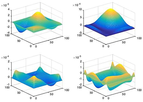
To illustrate the benefit of the distributed consensus filter proposed in this paper, we provide a simulated scenario in this section. Take into consideration an array of 2D spatially distributed processes with $Q(0,\theta )=\sin \left(\frac{\pi }{2}\theta \right){\mathrm{e}}^{-9{\theta }^2},\theta =[0,1]\times [0,1]$ as their initial condition. Dirichlet boundary conditions are followed by the system. Figure 1 shows the states of 2D spatial processes at four different times.

Figure 1. The states of 2D parabolic system at four different moments.

The diffusion operator $a_0=0.006$. Bounded nonlinear function $f\left(Q\right(t,\theta \left)\right)=5.2\arctan \left(0.8Q\right(t,\theta \left)\right)$. Among the three mobile sensors considered in this system, the initial position of each sensor is determined as $\left({\theta }_{11}\right(0),{\theta }_{12}(0\left)\right)=(0.15,0.18),\left({\theta }_{21}\right(0),{\theta }_{22}(0\left)\right)=(0.5,0.58)$ and $\left({\theta }_{31}\right(0),{\theta }_{32}(0\left)\right)=(0.75,0.98)$. The spatial distribution of each mobile sensing device is provided by $\begin{array}{r}\phi (\theta ;{\theta }_i)=\{\begin{array}{ll}{\displaystyle \frac{1}{0.36}}& \mathrm{i}\mathrm{f}({\theta }_1,{\theta }_2)\in [{\theta }_{i1}-0.03,{\theta }_{i1}+0.03]\\ & \times [{\theta }_{i2}-0.04,{\theta }_{i2}+0.04],\\ 0& \mathrm{o}\mathrm{t}\mathrm{h}\mathrm{e}\mathrm{r}\mathrm{w}\mathrm{i}\mathrm{s}\mathrm{e}.\end{array}\end{array}$The probabilities are taken as $\overline{\gamma }=0.6$, ${\overline{\alpha }}_1=0.9,{\overline{\alpha }}_2=0.85$ and ${\overline{\alpha }}_3=0.8$. Figures 2–4 show the measurement output of mobile sensors with random data missing.

Figure 2. The measurement output of first mobile sensors with random data missing.

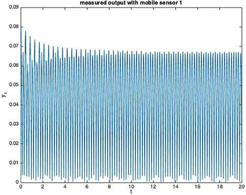
Figure 3. The measurement output of second mobile sensor with random data missing.

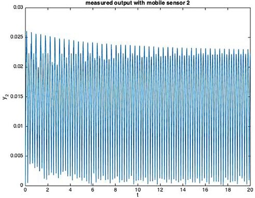
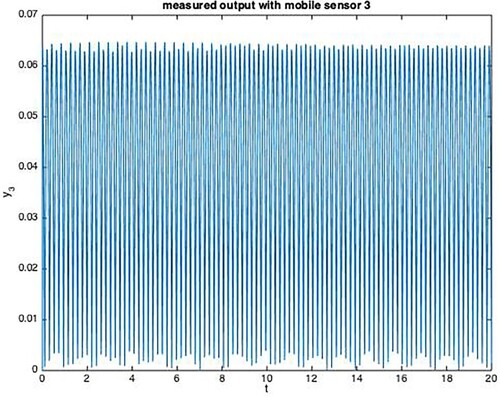
Figure 4. The measurement output of third mobile sensors with random data missing.

For the distributed consensus filter initial conditions are selected as ${\hat{Q}}_1(0,\theta )={\hat{Q}}_2(0,\theta )={\hat{Q}}_3(0,\theta )=0$. The filter gains are determined by $k_1=75,k_2=80$ and $k_3=70$.

Figures 5–7 depict the evolution of the filtering error system for the three distributed consensus filters.

Figure 5. The evolution of filtering error systems for filter 1.

Figure 6. The evolution of filtering error systems for filter 2.

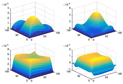
Figure 7. The evolution of filtering error systems for filter 3.

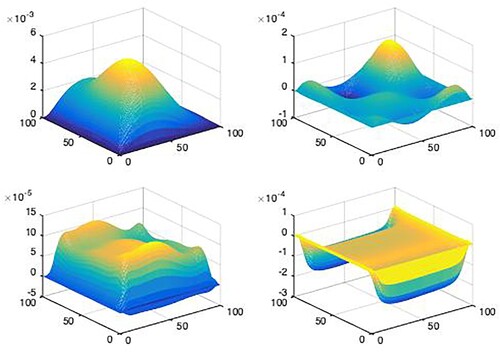
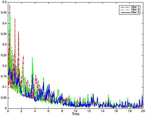
Figure 8 shows the evolution of $L_2$ norm for the three filtering error systems.

Figure 8. The evolution of $L_2$ norm for filtering error systems.

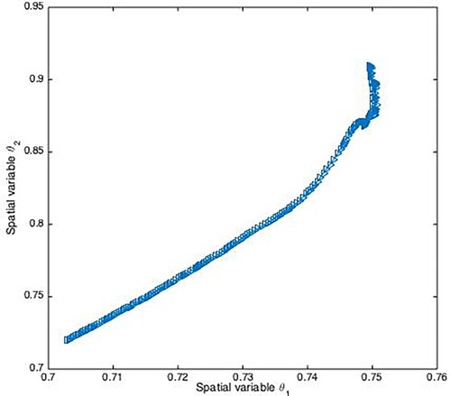
Three fixed-in-space sensors that are fixed at $({\theta }_{11},{\theta }_{12}=(0.15,0.18),({\theta }_{21},{\theta }_{22})=(0.5,0.58)$ and $({\theta }_{31},{\theta }_{32})=(0.75,0.98)$ are used as a comparison. Figure 9 shows the spatial trajectories of three sensors in both fixed and mobile scenarios. Also, Figures 10–12 show the moving paths of each mobile sensor in the 2D plane, respectively.

Figure 9. The trajectories of three mobile sensing devices.

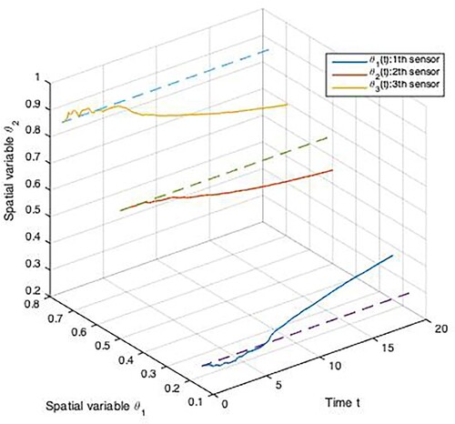
Figure 10. The trajectory of first mobile sensor.

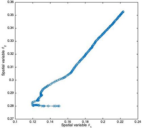
Figure 11. The trajectory of second mobile sensor.

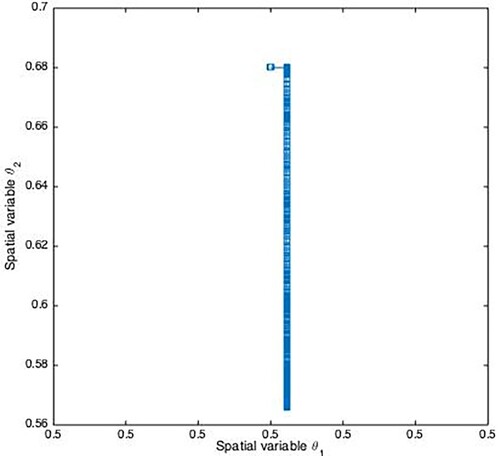
Figure 12. The trajectory of third mobile sensor.

5. Conclusions

A distributed consensus filter is designed in this paper for the consensus estimation using mobile sensor networks. Mobile sensing has been proposed as a novel optimal framework for improving filter performance in 2D parabolic systems with stochastic nonlinear function and bounded disturbances. The measurement output of each mobile sensor includes external noise. These noises are Brownian motions with a stochastic feature that meet the bounded sector assumption. The convergence of the filtering error system is affected by stochastic nonlinear and disturbance terms. Filtering errors only converge within certain bounds. Sufficient criterion for the uniformly bounded of the filtering error system has been established which used the operator-dependent Lyapunov functional, and an estimated bound has been presented. In addition, the velocity law of each mobile sensor can be adjusted such that the filtering error converges more faster to its bounds. The optimization framework proposed in this study under the mobile sensing approach allows for optimal performance of the filter design while explicitly incorporating the location of the mobile sensors into the process dynamics under this framework.

Disclosure statement

No potential conflict of interest was reported by the authors.

Additional information

Funding

This research was supported by the Natural Science Foundation of the Jiangsu Higher Education Institutions of China [No. 17KJB510051], Qing Lan Project of the Jiangsu Higher Education Institutions (Young and Middle-aged Academic Leader (2022), Excellent Teaching Team (2020)), Soft Science Research Project of Wuxi [No. KX-22-B60], Advanced Research and Study Project for Academic Leaders of Jiangsu Higher Vocational Colleges [No. 2021GRFX068], National Natural Science Foundation of China [61807016], Jiangsu Provincial Natural Science Foundation of China [BK20201340], China Postdoctoral Science Foundation [2018M642160].

Appendix 1.

Boundedness and coercivity of closed-loop operator

Considering the properties of the operator $\mathcal{A}$, the following calculation can be employed to prove that the closed-loop operator ${\mathcal{A}}_{\varphi }\left({\theta }_i\right(t\left)\right)$ satisfies the following properties: (A1) $\begin{array}{rl}& \left|\sum _{i=1}^N〈h,{\mathcal{A}}_{\varphi }\left({\theta }_i\right(t\left)\right)g〉\right|\\ & =\left|\sum _{i=1}^N〈h,(\mathcal{A}-k_i(1+{\delta }_i\left){\overline{\alpha }}_i{\Phi }_i^{\ast }\right({\theta }_i\left(t\right)\left){\Phi }_i\right({\theta }_i\left(t\right)\left)\right)g〉\right|\\ & \le {\alpha }_{0}N\Vert h\Vert \Vert g\Vert +〈h,K(1+\overline{\mathrm{\Delta }}){\overline{\mathrm{\Lambda }}}_{\alpha }{\Phi }^{\ast }\left(\theta \right(t\left)\right)\Phi \left(\theta \right(t\left)\right)g〉\\ & ={\alpha }_{0}N\Vert h\Vert \Vert g\Vert +〈K(1+\overline{\mathrm{\Delta }}){\overline{\mathrm{\Lambda }}}_{\alpha }\Phi \left(\theta \right(t\left)\right)h,\Phi \left(\theta \right(t\left)\right)g〉\\ & \le {\alpha }_{0}N\Vert h\Vert \Vert g\Vert +{\lambda }_{max}\left(K\right(1+\overline{\mathrm{\Delta }}\left){\overline{\mathrm{\Lambda }}}_{\alpha }\right)b^2{L}^2\left(S\right)\Vert h\Vert \Vert g\Vert \\ & =\alpha \Vert h\Vert \Vert g\Vert ,\end{array}$(A1) where $\alpha ={\alpha }_{0}N+{\lambda }_{max}\left(K\right(1+\overline{\mathrm{\Delta }}\left){\overline{\mathrm{\Lambda }}}_{\alpha }\right)b^2{L}^2\left(S\right)>0$, $\overline{\mathrm{\Delta }}=\mathrm{d}\mathrm{i}\mathrm{a}\mathrm{g}\{{\delta }_1,{\delta }_2,\dots ,{\delta }_N\}$, ${\overline{\mathrm{\Lambda }}}_{\alpha }=\mathrm{d}\mathrm{i}\mathrm{a}\mathrm{g}\{{\overline{\alpha }}_1,{\overline{\alpha }}_2,\dots ,{\overline{\alpha }}_N\}$, $K=\mathrm{d}\mathrm{i}\mathrm{a}\mathrm{g}\{k_1,k_2,\dots ,k_N\}$, $\Vert \Phi \left(\theta \right(t\left)\right)\Vert =bL\left(S\right)$. The above proof indicates that the boundedness of ${\mathcal{A}}_{\varphi }\left({\theta }_i\right(t\left)\right)$ is established. For coercivity, it is given by the following proofs: (A2) $\begin{array}{rl}& \sum _{i=1}^N〈h,-{\mathcal{A}}_{\varphi }\left({\theta }_i\right(t\left)\right)h〉\\ & =\sum _{i=1}^N〈h,-(\mathcal{A}-k_i(1+{\delta }_i\left){\overline{\alpha }}_i{\Phi }_i^{\ast }\right({\theta }_i\left(t\right)\left){\Phi }_i\right({\theta }_i\left(t\right)\left)\right)h〉\\ & \ge {\text{β}}_{0}N\Vert h{\Vert }^2+〈h,K(1+\overline{\mathrm{\Delta }}){\overline{\mathrm{\Lambda }}}_{\alpha }{\Phi }^{\ast }\left(\theta \right(t\left)\right)\Phi \left(\theta \right(t\left)\right)h〉\\ & ={\text{β}}_{0}N\Vert h{\Vert }^2+〈K(1+\overline{\mathrm{\Delta }}){\overline{\mathrm{\Lambda }}}_{\alpha }\Phi \left(\theta \right(t\left)\right)h,\Phi \left(\theta \right(t\left)\right)h〉\\ & \ge {\text{β}}_{0}N\Vert h{\Vert }^2+{\lambda }_{min}\left(K\right(1+\overline{\mathrm{\Delta }}\left){\overline{\mathrm{\Lambda }}}_{\alpha }\right)|\Phi \left(\theta \right(t\left)\right)h{|}^2\\ & >{\text{β}}_{0}N\Vert h{\Vert }^2.\end{array}$(A2)

References

- Chen, J., Tepljakov, A., Petlenkov, E., Chen, Y., & Zhuang, B. (2020). Observation and stabilisation of coupled time-fractional reaction–advection–diffusion systems with spatially-varying coefficients. IET Control Theory & Applications, 14(19), 3128–3138. https://doi.org/10.1049/cth2.v14.19
- Ding, D., Wang, Z., Dong, H., & Shu, H. (2012). Distributed H∞ state estimation with stochastic parameters and nonlinearities through sensor networks: The finite-horizon case. Automatica, 48(8), 1575–1585. https://doi.org/10.1016/j.automatica.2012.05.070
- Duan, J., Hu, M., Yang, Y., & Guo, L. (2014). A delay-partitioning projection approach to stability analysis of stochastic Markovian jump neural networks with randomly occurred nonlinearities. Neurocomputing, 128, 459–465. https://doi.org/10.1016/j.neucom.2013.08.019
- He, X., Wang, Z., & Zhou, D. (2007). Robust H∞ filtering for networked systems with multiple state delays. International Journal of Control, 80(8), 1217–1232. https://doi.org/10.1080/00207170701196968
- Hidayat, Z., Babusˇka, R., De Schutter, B., & Nu´n~ez, A.. (2011). Decentralized Kalman filter comparison for distributed-parameter systems: A case study for a 1D heat conduction process. ETFA2011, Toulouse, France, pp. 1–8. https://doi.org/10.1109/ETFA.2011.6059054
- Hu, J., Wang, Z., Gao, H., & Stergioulas, L. K. (2012). Extended Kalman filtering with stochastic nonlinearities and multiple missing measurements. Automatica, 48(9), 2007–2015. https://doi.org/10.1016/j.automatica.2012.03.027
- Li, Q., Shen, B., Wang, Z., & Sheng, W. (2020). Recursive distributed filtering over sensor networks on Gilbert–Elliott channels: A dynamic event-triggered approach. Automatica, 113, 108681. https://doi.org/10.1016/j.automatica.2019.108681
- Liu, Q., Wang, Z., He, X., & Zhou, D. H. (2015). Event-based recursive distributed filtering over wireless sensor networks. IEEE Transactions on Automatic Control, 60(9), 2470–2475. https://doi.org/10.1109/TAC.2015.2390554
- Liu, Y., Wang, Z., & Wang, W. (2011). Reliable H∞ filtering for discrete time-delay systems with randomly occurred nonlinearities via delay-partitioning method. Signal Processing, 91(4), 713–727. https://doi.org/10.1016/j.sigpro.2010.07.018
- Meditch, J. S. (1971). Least-squares filtering and smoothing for linear distributed parameter systems. Automatica, 7(3), 315–322. https://doi.org/10.1016/0005-1098(71)90123-3
- Nahi, N. (1969). Optimal recursive estimation with uncertain observation. IEEE Transactions on Information Theory, 15(4), 457–462. https://doi.org/10.1109/TIT.1969.1054329
- Omatu, S., & Seinfeld, J. H. (1981). Filtering and smoothing for linear discrete-time distributed parameter systems based on Wiener–Hopf theory with application to estimation of air pollution. IEEE Transactions on Systems, Man, and Cybernetics, 11(12), 785–801. https://doi.org/10.1109/TSMC.1981.4308618
- Sakawa, Y. (1972). Optimal filtering in linear distributed-parameter systems. International Journal of Control, 16(1), 115–127. https://doi.org/10.1080/00207177208932247
- Shen, B., Wang, Z., & Hung, Y. S. (2010). Distributed H∞-consensus filtering in sensor networks with multiple missing measurements: the finite-horizon case. Automatica, 46(10), 1682–1688. https://doi.org/10.1016/j.automatica.2010.06.025
- Shen, B., Wang, Z., Shu, H., & Wei, G. (2010). Robust H∞ finite-horizon filtering with randomly occurred nonlinearities and quantization effects. Automatica, 46(11), 1743–1751. https://doi.org/10.1016/j.automatica.2010.06.041
- Shen, B., Wang, Z., Shu, H., & Wei, G. (2011). H∞ filtering for uncertain time-varying systems with multiple randomly occurred nonlinearities and successive packet dropouts. International Journal of Robust and Nonlinear Control, 21(14), 1693–1709. https://doi.org/10.1002/rnc.1662
- Ugrinovskii, V., & Fridman, E. (2014). A Round-Robin type protocol for distributed estimation with H∞ consensus. Systems & Control Letters, 69, 103–110. https://doi.org/10.1016/j.sysconle.2014.05.001
- Wang, Z., Yang, F., Ho, D. W., & Liu, X. (2005). Robust finite-horizon filtering for stochastic systems with missing measurements. IEEE Signal Processing Letters, 12(6), 437–440. https://doi.org/10.1109/LSP.2005.847890
- Wei, G., Wang, Z., & Shu, H. (2009). Robust filtering with stochastic nonlinearities and multiple missing measurements. Automatica, 45(3), 836–841. https://doi.org/10.1016/j.automatica.2008.10.028
- Xu, C., Yu, F., & He, D. (2022). Disturbance-blocking-based distributed receding horizon estimation of flexible joint robots. Journal of Shanghai Jiaotong University, 56(7), 868–876. https://doi.org/10.16183/j.cnki.jsjtu.2021.186
- Yu, H., Zhuang, Y., & Wang, W. (2013). Distributed H∞ filtering in sensor networks with randomly occurred missing measurements and communication link failures. Information Sciences, 222, 424–438. https://doi.org/10.1016/j.ins.2012.07.059
- Yu, W., Chen, G., Wang, Z., & Yang, W. (2009). Distributed consensus filtering in sensor networks. IEEE Transactions on Systems, Man, and Cybernetics, Part B (Cybernetics), 39(6), 1568–1577. https://doi.org/10.1109/TSMCB.2009.2021254
- Zhang, D., Nguang, S. K., Srinivasan, D., & Yu, L. (2017). Distributed filtering for discrete-time T–S fuzzy systems with incomplete measurements. IEEE Transactions on Fuzzy Systems, 26(3), 1459–1471. https://doi.org/10.1109/TFUZZ.91
- Zhang, D., Shi, P., Zhang, W. A., & Yu, L. (2016). Energy-efficient distributed filtering in sensor networks: A unified switched system approach. IEEE Transactions on Cybernetics, 47(7), 1618–1629. https://doi.org/10.1109/TCYB.2016.2553043