Retailer involvement in carbon emission reduction under the Cap-and-Trade mechanism

ABSTRACT

Under the ‘ Cap-and-Trade’ mechanism of carbon emission, the low carbon management of supply chain is an indispensable link in the process of enterprise emission reduction. Constrained by carbon price and consumers’ environmental awareness, this paper establishes a two-stage game model between retailers and manufacturers under decentralized and centralized decisions. Under the decentralized decision, this paper analyzes the optimal carbon emissions before and after the transfer, the conditions of transfer and the changes of profits with the proportion of transfer. Under the centralized decision, Nash equilibrium is used to study the distribution of additional profits. Conclusions are obtained as follows. (a) There are thresholds for carbon price and consumers’ environmental awareness on carbon emissions, and the optimal emissions on both sides of the threshold will vary with the cost of emission reduction. (b) In a decentralized decision, the participation of retailers in abatement depends on the market abatement costs and abatement benefits, while a certain range of transfer rates can optimize the profitability of retailers. (c) In the centralized decision, manufacturer and retailer formulate emission reduction strategies jointly and share the extra profits equally.

KEYWORDS:

• Cap-and-Trade
• carbon emission
• consumer environmental awareness
• decentralized decision
• centralized decision

1. Introduction

Most scientists and governments acknowledge that greenhouse gases have been and will continue to bring disasters to the earth and mankind. In recent years, environmental legislation has gradually changed from traditional command and control policy to market-based tools. For the resolution of the environmental problem, the European Union has taken the lead in establishing a ‘Cap-and-Trade’ system, which requires member states to reduce the quota allocation of enterprises gradually and increase the proportion of carbon emissions auctions. This system has changed the traditional way of enterprises’ development, leading them to carry out the environmental concept of low carbon. Because of the worldwide supply chain, carbon consumption spreads all over the world, and its negative effects, such as carbon emissions and pollution, have attracted wide attention. With the constraint of low carbon, it is of great significance to formulate the optimal emission reduction strategy for the traditional supply chain. The trade-off between economic objectives and environmental sustainability is a key issue in supply chain’s management (Clarke et al., 2017; Lam et al., 2013). Therefore, it is necessary to take environmental factors into consider when making decisions of supply chain (Brandenburg et al., 2019; Kuo et al., 2014; 2018; Xu et al., 2020).

To reduce carbon emission, the enterprises have to consume plenty of manpower, material and financial resource, which increases enterprise costs and reduces benefits. In order to promote the emission reduction of enterprises, countries have implemented various low-carbon policies. As the common policy of carbon emission reduction, the ‘Cap-and-Trade’ mechanism aims to impose carbon’s quota on high-emission enterprises (Kumar et al., 2015; Singh et al., 2019). Thus it forces enterprises to develop emission reduction technologies (Huang, Wang, et al., 2019; Yu et al., 2020). Under that mechanism, policies and consumer environmental awareness have deep influences on the decision of emission reduction in the supply chain, which is shown as follows: in terms of government policies, carbon policies affect business decisions, such as investment in emission reduction (Ganda, 2019; Qiao et al., 2019); in terms of consumer environmental awareness, consumers who are sensitive to carbon make the production decisions of enterprises more complicated (Dong & Bi, 2020; Liu et al., 2021; Lopes de Sousa Jabbour et al., 2021).

Within different decisions, the formulation and implementation of emission reduction tasks have lots of differences. Under the decentralized decision, manufacturers and retailers, as independent individuals, make decisions based on their own interests. In setting the task of carbon emission reduction, the manufacturer makes decisions, and the retailer can get a ‘free ride’ and gain profits, so that the retailer also need to participate in emission reduction actively. But an interval for the transfer of carbon emission tasks is needed, and too little or too much is not conducive to the stability of the supply chain. Under the centralized decision, the manufacturer and the retailer work together as a group to implement emission reduction tasks, to formulate unified emission reduction strategies and to distribute the overall revenue jointly.

At present, the research on low-carbon supply chain mainly focuses on three aspects: (1) the researches on low-carbon policy, which mainly focus on carbon tax, carbon emission disclosure policy and its impact on emission reduction and enterprise decision-making; (2) the researches on enterprise emission reduction mechanism, which mainly focus on enterprise inventory management, supply chain management and emission reduction cooperation strategies between manufacturers and retailers; (3) the researches on consumer environmental awareness, which mainly focus on consumers’ environmental preference on enterprises’ decision. However, there are very few studies on the transfer and emission reduction tasks arising from carbon emission policies, and even fewer studies on the transfer and emission reduction task mechanism and the limits of the retailer’s responsibility in the supply chain. This paper mainly explores the transfer of carbon emission tasks in the supply chain, clarifies the conditions and degree of transfer under different decisions and deepens the research on low-carbon supply chain management.

This paper is organized as follows: Section 1 introduces the background and significance of low-carbon supply chain management and many carbon emission transfer strategies. Section 2 reviews the relevant literature and introduces the main contribution of this study. Section 3 constructs a two-stage game model for manufacturers and retailers under different decisions, and explains assumptions and symbols. Section 4 analyses the profit functions of the manufacturer and the retailer under different decisions determines the best time and the best transfer degree of the retailer to undertake carbon emission tasks, so as to achieve the overall optimization of the supply chain. Section 5 uses MATLAB software to simulate and reflect the research results more intuitively. Section 6 summarizes the relevant conclusions and the management significance.

2. Literature review

This section mainly reviews the literature relevant to this study, and there are three main relevant literature streams: (1) research on the impact of the carbon ‘Cap-and-Trade’ mechanism on supply chain. (2) Research on the impact of government policies and consumer environmental awareness on the formulation of supply chain emission reduction strategies. (3) Research on the current situation of carbon emission transfer.

2.1. The impact of the carbon ‘Cap-and-Trade’ system on supply chain

The carbon ‘Cap-and-Trade’ system affects the supply chain management and operation of enterprises. When a carbon cap is placed on an enterprise, the enterprise will convey the impact to the whole value chain by virtue of the value chain (Busch & Hoffmann, 2007). Owning to the constraint of the carbon cap, the enterprise needs to consider the final emission of the product, which may include investigating the emission of upstream suppliers to select suppliers with lower emissions, and may also transfer carbon emissions of the downstream enterprises, so as to realize ‘green washing’ for themselves. In the context of joint information asymmetry and the Cap-and-Trade mechanism, Yuan et al. (2018) designed an incentive contract to make the manufacturer disclose the carbon information. Suppliers could also transfer the cost of green investment to consumers through retailers, thus achieving both economic and environmental benefits (Barari et al., 2012). The authors explored that relevant manufacturers held multiple products, which met the carbon emission regulation of joint production and pricing (Huang, Hu, et al., 2019; Xu et al., 2016). In general, the carbon constraint has been defined as three categories: policy-driven, market-driven and nature-driven. In the process of operation, the main consideration is policy-driven, and the scheme ranks first and the tax second. In addition, the policymakers can learn about business decisions to reduce carbon emissions and make proper use of emission reduction incentives (P. Zhou & Wen, 2020). Cap-and-Trade has become one of the most widely used carbon emission limitation methods in the world. Its constraints have a great impact on the carbon emission reduction decisions and production operations of supply chain enterprises, as well as profit distribution (Jiang et al., 2019).

2.2. The impact of emission reduction policy of supply chain under dual constraints

Carbon policy, as one of the important means to realize the carbon quota mechanism, will affect business decisions of enterprises, such as investment in emission reduction technology (Wang & Wu, 2021). The behaviour strategies of supply chain participants are mainly influenced by government policies, and the government also needs to make some dynamic strategic adjustments in response. The research results of Xu et al. (2018) showed that the Cap-and-Trade system established by government can effectively reduce carbon emissions and achieve coordinated development of economy and environment. Madani and Rasti-Barzoki (2017) studied the impact of low-carbon subsidies and carbon tax policies on supply chain performance and social benefits. They argued that government decisions on subsidies and taxes could increase the sustainability of decisions determined by the supply chain. Ding et al. (2016) explored decision-making mechanism of environmental sustainability supply chain, which is not only restricted by the environmental carrying capacity, but also by the emission cap, and stimulated by government policies. Chen and Hu (2018) found that the carbon tax imposed by government was more effective in encouraging low-carbon manufacturing than the subsidies for low-carbon technologies. Since the central intention of planner is to reduce carbon emissions in different industries at different levels of competition, Wen et al. (2018) argued that raising consumer awareness maybe not an excellent choice. Da et al. (2019) found that the high bank loan discount rate for investing in carbon reduction technology equates to large carbon reduction in coal enterprises.

With the improvement of environmental protection awareness of consumers, the market choice of consumers has gradually become an important social mechanism to restrain the negative externalities of enterprise environment. The environmental awareness of consumers is mainly formed in response to resource waste, non-renewable resources, environmental pollution and other problems in economic development, as well as changes in the consumption concepts and behaviours of them (Lian et al., 2018; Zhou et al., 2020). Borin et al. (2013) investigated whether the green strategy will influence the purchase intentions of consumers. They concluded that consumers were significantly more likely to buy green products than non-green ones, and they expected to pay high prices for the former due to their environmental awareness (Shewmake et al., 2015). Nouira et al. (2016) found that the environmental awareness of customers may lead enterprises to close the production area to the consumption area, as well as to choose local suppliers. If customers have high demand for low carbon, the best strategy is to design a supply chain with relatively high emission level. Improving consumers’ awareness of environmental protection, although not at higher profits for manufacturers, will encourage manufacturers to produce more green products. Consumers’ environmental awareness will also affect the government's carbon price subsidies. When consumer prices are sensitive, the government’s optimal subsidy intensity increases as consumers’ low-carbon preferences increase. When consumer prices are not sensitive, the government should not provide any subsidies (Zhang et al., 2020).

2.3. The current research of carbon emission transfer

The existence of international trade contributes to the continuous expansion of production and consumption activities, as well as the realization of cross-border regional division, which leads to the regional transfer of global carbon emissions (López et al., 2018; Sun et al., 2016). The developed economies in the upstream of the global value chain tend to outsource their emission intensive production activities to countries with loose environmental standards, while the developing economies in the lower reaches of the global value chain specialize in energy intensive processing and manufacturing activities, which leads to an increase in global carbon emissions (Cai et al., 2018). Guan and Reiner (2009) found that about a quarter of the gas emissions from developing countries came from developed countries with which they had commodity trade relations. This phenomenon has led to an increase in carbon emissions of developing countries. At present, most of the carbon emission transfer problems studied by scholars can be divided into three types: international carbon emission transfer (Li et al., 2018; Zhengning et al., 2020), provincial carbon emission transfer (Fan et al., 2019; Liu et al., 2018) and inter-industrial carbon emission transfer (Xu et al., 2019). Li et al. (2018) studied the carbon emissions of four municipalities in China, which found that the four municipalities, as the bridge of carbon transfer between China and other countries, were the key nodes to balance the rapid economic growth and environmental sustainability of foreign economies and domestic provinces. Zhengning et al. (2020) used structural decomposition analysis to explore the driving factors reflecting carbon emission changes in international and provincial trade. Su and Ang (2010) analysed the specific transfer of China through the differences among different provinces in China. Hou et al. (2020) calculated the actual carbon transfer in 28 industries and established a visual dynamic carbon database to describe and analyse the specific carbon transfer structure among different industries in China.

Based on literature discussed above, we can find that the carbon quota mechanism does have a significant impact on supply chain emission reduction, and the main influencing factors are government policies and consumer environmental awareness. However, most of the current researches on carbon emission transfer mainly focus on the carbon emission transfer among countries, provinces or industries. These studies suggest that retailers should undertake the transfer of carbon emissions from manufacturers, but they do not specify retailers’ commitment. In addition, there are also a few studies on the boundaries of manufacturers’ transfer of carbon emission tasks under the decentralized and centralized decisions.

In order to clarify the conditions of carbon emission transfer, this paper studies the decentralized and centralized decision process of the retailer and the manufacturer under the dual constraints of policy and consumer environmental awareness. It analyses: (1) the change and transfer conditions of carbon emissions before and after the transfer of emission reduction under the decentralized decision; (2) the state of each variable with the transfer proportion of emission reduction and the transfer proportion corresponding to the optimal decision under the decentralized decision and (3) the distribution game of extra profit under the centralized decision.

3. Model assumptions

We assumed that there is only one manufacturer and one retailer in the market, and the manufacturer is in a dominant position. As the manufacturer formulated a strategy, the retailer was forced to accept it. Consumer’s behaviour can influence the decisions of the manufacturer and the retailer, and the manufacturer can transfer emission reduction tasks to retailers by some strategies, such as the retailer undertaking transportation process, the manufacturer expanding the inventory of retailers and requiring retailers to book goods in advance. Meanwhile, retailers can receive an additional ‘price premium’ on account of consumer environmental awareness and benefit from manufacturers’ emission reduction strategies. Therefore, retailers are willing to undertake a certain proportion of emission reduction tasks and promote the reduction of carbon emissions of products. For manufacturers, the reduction of carbon emissions will lead to an increase in sales, which will benefit manufacturers.

There is a threshold constraint on the sharing of emission reduction tasks between manufacturers and retailers, and both sides make optimal decisions based on the maximization of their own profits. Manufacturers can not transfer emission reduction tasks to retailers without restriction, and when the cost of emission reduction tasks undertaken by retailers greatly exceeds the benefits, retailers will transfer emission reduction costs to consumers by increasing retail prices. This phenomenon will lead to decrease in sales, which will reverse the profits of manufacturers. This paper establishes a two-stage game model to study the proportion of supply chain transfer tasks.

The notations used in the model are described in Table 1.

Table 1. Model notations.

Symbol	Definition
$Q$	Consumer demand
$Q^{\ast }$	The optimal demand
$a$	The scale of production
$p$	Retail price
$w$	Wholesale price
$c$	Manufacturing cost
$k$	Consumer’s sensitivity to the emissions of the product
$E$	Emission per unit product
$E_0$	Initial emission per unit product
$E_{cap}$	Emissions cap
$p_c$	Carbon price
$t$	Cost coefficient for manufacturers to deal with unit emissions
$C_c$	Emission reduction costs of manufactures under decentralized decision
${\prod }_r^d\left(p\right)$	The benefit function of retailers under decentralized decision without transfer
${\prod }_m^d(w,E)$	The benefit function of manufacturers under decentralized decision without transfer
${\prod }_r^{d\text{β}}\left(p\right)$	The benefit function of retailers under decentralized decision with transfer
${\prod }_m^{d\text{β}}(w,E)$	The benefit function of manufacturers under decentralized decision with transfer
$\alpha$	Proportion undertaken by retailers
$\text{β}$	Proportion undertaken by manufacturers, $\text{β}=1-\alpha$
$E_d^{\ast }$	Optimal carbon emissions under decentralized decision without transfer
$E_{d\text{β}}^{\ast }$	Optimal carbon emissions under decentralized decision with transfer
$E_s^{\ast }$	Optimal carbon emissions under centralized decision
${\prod }_s^{}(p,E)$	The benefit function under centralized decision
$u_m(w,\text{β})$	Utility of manufacturers under centralized decision
$u_r(w,\text{β})$	Utility of retailers under centralized decision
$u_m^{\ast }$	Optimal utility of manufacturers under centralized decision
$u_s^{\ast }$	Optimal utility of retailers under centralized decision
$w_s^{\ast }$	Internal optimal wholesale price under centralized decision

Assumption 3.1:

There is only one manufacturer and one retailer in the market, and the manufacturer in a dominance. Thus the retailer is forced to accept the manufacturer's decision. If the manufacturer wants to transfer the carbon emission task, the proportion of manufacturer is $\text{β}$, and that of the retailer is $\alpha =1-\text{β}$. As it is impossible to move all the emission reduction tasks, the proportion can be shown as 0≤$\text{β}$<1.

Assumption 3.2:

Due to consumer environmental awareness, the decision variable $E$ is introduced into the demand function, and the carbon emission is negatively correlated with product demand. Referring to the demand function of Yalabik and Fairchild (2011), it is expressed as follows: $Q=a-p-kE$In which, $kE$ is the market reaction of consumers to the carbon emission for per unit of product $E$, that is, when E decreases, consumer demand will rise.

Assumption 3.3:

Assume that the price of carbon $p{}_c$ is a constant.

Assumption 3.3:

Referring to the cost function of Yalabik and Fairchild (2011), if the carbon emission of per unit product reduces from $E_0$ to $E$, the cost of carbon emission can be expressed as $C_c=t(E_0-E{)}^2$.

Within this modeling framework, we can establish a two-stage game model that the retailer’s and manufacturer’s revenue functions as follows: the retailer’s revenue function is (1) $\begin{array}{r}{\prod }_r^{}\left(p\right)=(p-w)Q-t\alpha (E_0-E{)}^2\end{array}$(1) and the manufacturer’s revenue function is (2) $\begin{array}{r}{\prod }_m^{}(w,E)=(w-c)Q-t\text{β}(E_0-E{)}^2-p_c(EQ-E_{cap})\end{array}$(2)

4. Analysis

4.1. The carbon emission strategy of manufacturers under the decentralized decision

In the decentralized decision-making, both the manufacturer and the retailer make decisions to maximize their own interests. In this case, when the manufacturer does not transfer the carbon emission task to the retailer, the profit function of the retailer can be expressed as follows: (3) $\begin{array}{r}{\prod }_r^d\left(p\right)=(p-w)Q\end{array}$(3) The profit function of the manufacturer can be expressed as (4) $\begin{array}{rl}{\prod }_m^d(w,E)& =(w-c)Q-t(E_0-E{)}^2\\ & -p_c(EQ-E_{cap})\cdot \cdot \text{s}\text{.t}.0\le E\le E_0\end{array}$(4)

Theorem 4.1:

When the manufacturer does not transfer the carbon emission task to the retailer, the optimal carbon emission under different circumstances is as follows:

1. If $p_c+k\ge \frac{a-c}{E_0}$ and $t>\frac{{(p_c+k)}^2}{8}$ or $p_c+k\le \frac{a-c}{E_0}$ and $t<\frac{{(p_c+k)}^2}{8},E_d^{\ast }=E_0^{}$.

2. If $p_c+k\ge \frac{a-c}{E_0}$ and $t<\frac{(p_c+k)(a-c)}{8E_0}$ or $p_c+k<\frac{a-c}{E_0}$ and $t>\frac{(p_c+k)(a-c)}{8E_0},E_d^{\ast }=\frac{8t{E}_0-(a-c)(p_c+k)}{8t-{(p_c+k)}^2}$.

3. If $p_c+k>\frac{a-c}{E_0}$ and $\frac{{(p_c+k)}^2}{8}>t\ge \frac{(p_c+k)(a-c)}{8E_0}$ or $p_c+k<\frac{a-c}{E_0}$ and $\frac{(p_c+k)(a-c)}{8E_0}\ge t\frac{{(p_c+k)}^2}{8},E_d^{\ast }=0$.

The process is shown in proof 4.1.

Its conclusions are shown in the coordinate system as follows.

The $p_c+k$ represents the comprehensive constraint of policy and consumer environmental awareness. Since $a,c$ and $E_0$ are constants, the threshold $(a-c)/E_0$ representing $p_c+k$ is also constant, and its corresponding value of $t$ is $(a-c{)}^{\text{2}}/\text{8}{E}_{\text{0}}^{\text{2}}$.

Enterprises that participate in emission reduction constraints are divided into two parts: one is those who have invested in emission reduction and the other is those who have not.

The optimal constraint for the enterprises that have invested in emission reduction is region $A_1$. In the process of emission reduction, with the emission becoming smaller and smaller, the difficulty of emission reduction is getting higher and higher, and the investment in emission reduction technology is increasing. For enterprises, if the constraints of policies and consumer environmental awareness are further improved, the benefits brought by emission reduction are less than the investment in emission reduction, which will lead to decrease in enterprises’ willingness for emission reduction. When $p_c+k$ further exceeds $(a-c)/E_0$, that is, when the enterprise’s investment in emission reduction is equal to or greater than its income, the enterprise will no longer invest in emission reduction. At this time, the most emission decision of the enterprise is the initial value $E_0$.

The optimal constraint for the enterprise that have not invested in emission reduction is region $A_2$. Because the enterprise has no willingness to invest in emission reduction, the comprehensive constraints of policy and consumer environmental awareness need to be greater than the threshold value $(a-c)/E_0$ so as to promote enterprises to invest in emission reduction. When the enterprise invests in emission reduction and continue to expand their investment, their optimal carbon emissions enter region $A_1$.

In the decentralized decision, the manufacturer can transfer part of the carbon emission task to the retailer, and the transfer proportion is $\alpha =1-\text{β}$.

At this point, the profit function of the retailer can be expressed as (5) $\begin{array}{r}{\prod }_r^{d\text{β}}\left(p\right)=(p-w)Q-t(1-\text{β})(E_0-E{)}^2\end{array}$(5) The profit function of the manufacturer can be expressed as (6) $\begin{array}{rl}{\prod }_m^{d\text{β}}(w,E)& =(w-c)Q-t\text{β}(E_0-E{)}^2\\ & -p_c(EQ-E_{cap})\text{s}\text{.t}.\cdot 0\le E\le E_0\end{array}$(6)

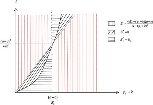
Theorem 4.2:

When the manufacturer transfers the carbon emission task to the retailer and the proportion is $\text{β}$, the optimal carbon emission under different circumstances is as follows:

1. If $p_c+k\ge \frac{a-c}{E_0}$ and $t>\frac{{(p_c+k)}^2}{8\text{β}}$ or $p_c+k\le \frac{a-c}{E_0}$ and $t<\frac{{(p_c+k)}^2}{8\text{β}},E_{d\text{β}}^{\ast }=E_0^{}$.

2. If $p_c+k\ge \frac{a-c}{E_0}$ and $t<\frac{(p_c+k)(a-c)}{8\text{β}{E}_0}$ or $p_c+k<\frac{a-c}{E_0}$ and $t>\frac{(p_c+k)(a-c)}{8\text{β}{E}_0},E_{d\text{β}}^{\ast }=\frac{8t\text{β}{E}_0-(a-c)(p_c+k)}{8t\text{β}-{(p_c+k)}^2}$.

3. If $p_c+k>\frac{a-c}{E_0}$ and $\frac{{(p_c+k)}^2}{8\text{β}}>t\ge \frac{(p_c+k)(a-c)}{8\text{β}{E}_0}$ or $p_c+k<\frac{a-c}{E_0}$ and $\frac{(p_c+k)(a-c)}{8\text{β}{E}_0}\ge t\frac{{(p_c+k)}^2}{8\text{β}},E_{d\text{β}}^{\ast }=0$.

The process is shown in proof 4.2.

Its conclusions are shown in the coordinate system as follows.

As we can be seen from Figures 1–2, the threshold value $p_c+k$ of comprehensive constraint remains unchanged with transfer under the decentralized decision, which is still $(a-c)/E_0$. However, the optimal emissions $E_{d\text{β}}^{\ast }$ and the cost coefficient $t$ corresponding to the threshold value have changed.

Figure 1. Optimal emissions without transfer under the decentralized decision.

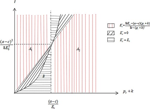
Figure 2. Optimal emissions with transfer under decentralized decision.

The value of $t$ becomes $(a-c{)}^{\text{2}}/\text{8}\text{β}{E}_{\text{0}}^{\text{2}}$ and the value of $E_{d\text{β}}^{\ast }$ becomes $[8t\text{β}{E}_0-(a-c\left)\right(p_c+k\left)\right]/[8t\text{β}-(p_c+k{)}^2]$. Therefore, we make a conclusion that the manufacturer’s emission reduction cost $t$ corresponding to the threshold value increases. When the manufacturer has fewer emission reduction tasks, the emission reduction funds will be invested in fewer emission reduction tasks. It will lead to an increase in the input of emission reduction tasks per unit and more in-depth research and development of emission reduction technologies.

Theorem 4.3:

Given $\text{β}<1$, the manufacturer should choose to transfer the carbon emission task when:

1. $p_c+k\ge \frac{a-c}{E_0}$ and $\text{β}\le \frac{a-c}{E_0(p_c+k)}$ and $t\ge \frac{{(p_c+k)}^2}{8}$.

2. $p_c+k\ge \frac{a-c}{E_0}$ and $\text{β}\ge \frac{a-c}{E_0(p_c+k)}$ and $t\ge \frac{(a-c)(p_c+k)}{8\text{β}{E}_0}$.

3. $p_c+k\le \frac{a-c}{E_0}$ and $t<\frac{{(p_c+k)}^2}{8}$ or $t\ge \frac{{(p_c+k)}^2}{8\text{β}}$.

There are $E_{d\text{β}}^{\ast }\le E_d^{\ast }$ at this time.

The process is shown in proof 4.3.

According to Theorems 4.1 and 4.2, the value of $E_{d\text{β}}^{\ast }$ and $E_d^{\ast }$ under different decisions are discussed respectively. It can be seen that the size relation between $E_{d\text{β}}^{\ast }$ and $E_d^{\ast }$ is determined by $p_c+k$, $\text{β}$ and $t$. Based on the emission reduction cost of the manufacturer, the government can formulate a more detailed carbon disclosure policy, and adjust the carbon price to make the optimal emission reduction of the whole supply chain smaller by understanding the proportion of transfer tasks.

Theorem 4.4:

In the decentralized system, when the carbon emission task is transferred, the optimal indexes change with $\text{β}$ as follows:

1. The optimal emission $E_{d\text{β}}^{\ast }$ increases as $\text{β}$ increases.

2. If $p_c>k$, the optimal wholesale price $w_{d\text{β}}^{\ast }$ increases as $\text{β}$ increases; if $p_c<k$, the optimal wholesale price $w_{d\text{β}}^{\ast }$ decreases with the increase in $\text{β}$.

3. The optimal sales Q decreases as $\text{β}$ increases.

4. If $1-\text{β}<(p_c+k{)}^2/16t$, the optimal profit of the retailer $\prod _r^{d\text{β}\ast }\left(p\right)$ decreases as $\text{β}$ increases; if $1-\text{β}>(p_c+k{)}^2/16t$, the optimal profit of the retailer $\prod _r^{d\text{β}\ast }\left(p\right)$ increases as $\text{β}$ decreases.

5. The optimal profit of the manufacturer $\prod _m^{d\text{β}\ast }(w,E)$ decreases as $\text{β}$ increases.

The process is shown in proof 4.4.

For the manufacturer, the optimal emission reduction will increase with the increase in emission reduction tasks, but their profits will decrease accordingly. When the carbon price is high, if the manufacturer undertakes more emission reduction tasks, the manufacturer will make a strategy to increase the wholesale price. When the carbon price is low, if the manufacturer undertakes the higher emission reduction task, the manufacturer will make the strategy to decrease the wholesale price. Therefore, in order to keep the overall emission reduction effect of the supply chain better, we should raise the carbon price under the threshold constraint, and urge the manufacturer to transfer the emission reduction task.

For the retailer, $1-\text{β}<(p_c+k{)}^2/16t$ means that the proportion undertaken by the retailer is less than $(p_c+k{)}^2/16t$, and the profit of retailers decreases with the increase in $\text{β}$, which can be explained that increased emissions reductions by manufacturers will lead to lower sales and thus lower profits for retailers. When the proportion undertook by the retailer is greater than $(p_c+k{)}^2/16t$, the less emission reduction task the retailer undertakes, the more profit the retailer can make by ‘free riding’. Therefore, when it is $\alpha =(p_c+k{)}^2/16t$, the retailer can get the maximum profit.

4.2. The carbon emission strategy of a manufacturer under the centralized decision

The manufacturer and the retailer form a unified whole to discuss relevant economic strategies under the centralized decision, to minimize the common total cost of both parties, so as to achieve the optimal overall benefits of the supply chain. In the process of making plans to reducing emission, the unified whole can make decisions, and the profit function of the whole system can be expressed as (7) $\begin{array}{rl}{\prod }_s^{}(p,E)& =(p-c)Q-t(E_0-E{)}^2\\ & -p_c(EQ-E_{cap})\cdot \cdot s.t.\cdot 0\le E\le E_0\end{array}$(7)

Theorem 4.5:

In the centralized system, the optimal carbon emission under different conditions is as follows:

1. If $p_c+k\ge \frac{a-c}{E_0}$ and $t>\frac{{(p_c+k)}^2}{4}$, or $p_c+k\le \frac{a-c}{E_0}$ and $t<\frac{{(p_c+k)}^2}{4}$ $E_s^{\ast }=E_0$

2. If $p_c+k<\frac{a-c}{E_0}$ and $\frac{{(p_c+k)}^2}{4}<t\le \frac{(p_c+k)(a-c)}{4E_0}$, or $p_c+k>\frac{a-c}{E_0}$ and $\frac{(p_c+k)(a-c)}{4E_0}<t\le \frac{{(p_c+k)}^2}{4}$ $E_s^{\ast }=0$

3. If $p_c+k<\frac{a-c}{E_0}$ and $t\ge \frac{(p_c+k)(a-c)}{4E_0}$,or $p_c+k>\frac{a-c}{E_0}$ and $t<\frac{(p_c+k)(a-c)}{4E_0}$ $E_s^{\ast }=\frac{4t{E}_0-(p_c+k)(a-c)}{4t-{(p_c+k)}^2}$

The process is shown in proof 4.5.

Its conclusions are shown in the coordinate system as follows.

As we can be seen from Figure 3, the threshold value $p_c+k$ of comprehensive constraint remains unchanged under the centralized decision, which still remains $(a-c)/E_0$. However, the optimal emissions $E_{d\text{β}}^{\ast }$ and the cost coefficient$t$ corresponding to the threshold value have changed.

Figure 3. Optimal emission under centralized decision.

The $t$ becomes $(a-c{)}^{\text{2}}/\text{4}{E}_{\text{0}}^{\text{2}}$ and the $E_{d\text{β}}^{\ast }$ becomes $\frac{\text{4}t{E}_0-(a-c)(p_c+k)}{\text{4}t-{(p_c+k)}^2}$. It concludes that the manufacturer's emission reduction cost $t$ corresponding to the threshold value increases. That is, when the manufacturer has fewer emission reduction tasks, the emission reduction funds will be invested in fewer emission reduction tasks, which will lead to an increase in the input of emission reduction tasks per unit and more in-depth research and development of emission reduction technologies. This shows that the transfer of emission reduction tasks in the decentralized decision and the implementation of centralized decision can promote the in-depth research and development of enterprises’ emission reduction technologies.

4.3. The coordination of the supply chain

The previous section has indicated that, in order to pursue the best overall benefit of the supply chain, the retailer and the manufacturer should jointly set the wholesale price, and the profit distribution problem can be seen in Theorem 4.6.

Theorem 4.6:

In the centralized decision-making, the utility of manufacturer is as follows: (8) $\begin{array}{rl}{u}_m(w,\text{β})& =(w-c)Q_s^{\ast }-t\text{β}(E_0-E_s^{\ast }{)}^2\\ & -p_c(E_s^{\ast }{Q}_s^{\ast }-E_{cap})-\prod _m^{d\ast }\end{array}$(8) The utility of the retailer is as follows. (9) $\begin{array}{r}{u}_r(w,\text{β})=(p_s^{\ast }-w)Q_s^{\ast }-t(1-\text{β})(E_0-E_s^{\ast }{)}^2-\prod _r^{d\ast }\end{array}$(9) The optimal wholesale price $w^{\ast }$ and $\text{β}$ should satisfy Equation (10): (10) $\begin{array}{r}{w}_s^{\ast }=\frac{(p_s^{\ast }+c)Q_s^{\ast }-tA+B-C+D}{2Q_s^{\ast }}+\frac{tA}{Q_s^{\ast }}\text{β}\end{array}$(10) where $A=(E_0-E{)}^2,B=\prod _m^{d\ast },C=\prod _r^{d\ast },D=p_c(E_S^{\ast }{Q}_S^{\ast }-E_{cap})$.

Proof

for Theorem 4.6.

Both the manufacturer and the retailer will seek to maximize their own interests, and hope to obtain more additional revenue. This paper analyses the game process between them by coordinating supply chain. If the manufacturer and retailer accept this scheme, there is $u_m(w,\text{β})=u_r(w,\text{β})$. If one of them disagree, there will be $u_m(w,\text{β})<u_r(w,\text{β})$ and $u_m(w,\text{β})>u_r(w,\text{β})$. If both parties disagree, their cooperation will be cancelled, and the centralized decision will not work. At this time, there is $u_m(w,\text{β})=u_r(w,\text{β})=0$. The three situations above can be expressed in Table 2.

Table 2. Game model of manufacturer and retailer.

Retailer manufacturer	Accept	Reject
Accept	$u_m=u_r$	$u_m>u_r$
Reject	$u_m<u_r$	$u_m=u_r=0$

For a manufacturer, no matter how a retailer chooses, the acceptance of the manufacturer will bring greater profits, similarly, which will make the retailer more profitable. At this point, there is $u_m(w,\text{β})=u_r(w,\text{β})$. That is:

$(w-c)Q_s^{\ast }-t\text{β}(E_0-E_S^{\ast }{)}^2-p_c(E_S^{\ast }{Q}_S^{\ast }-E_{cap})-\prod _m^{d\ast }=(p_s^{\ast }-w)Q_s^{\ast }-t(1-\text{β})(E_0-E_S^{\ast }{)}^2-\prod _r^{d\ast }$ The optimal wholesale can be obtained as follows: $\begin{array}{rl}{w}_s^{\ast }& =\frac{\begin{array}{c}(p_s^{\ast }+c)Q_s^{\ast }-t{(E_0-E_S^{\ast })}^2\\ +\prod _m^{d\ast }-\prod _r^{d\ast }+p_c(E_S^{\ast }{Q}_S^{\ast }-E_{cap})\end{array}}{2Q_s^{\ast }}\\ & +\frac{t{(E_0-E_S^{\ast })}^2}{Q_s^{\ast }}\text{β}\\ & =\frac{(p_s^{\ast }+c)}{2}+\frac{+\prod _m^{d\ast }-\prod _r^{d\ast }+p_c(E_S^{\ast }{Q}_S^{\ast }-E_{cap})}{2Q_s^{\ast }}\\ & +\frac{t(2\text{β}-1){(E_0-E_S^{\ast })}^2}{2Q_s^{\ast }}\end{array}$And $u_m^{\ast }=u_r^{\ast }=\frac{\begin{array}{c}(p_s^{\ast }-c)Q_s^{\ast }-t{(E_0-E_S^{\ast })}^2\\ +\prod _m^{d\ast }-\prod _r^{d\ast }-p_c(E_S^{\ast }{Q}_S^{\ast }-E_{cap})\end{array}}{2}$As the supply chain coordination is implemented, the revenue of the whole supply chain increases, and the manufacturer and retailer can obtain additional benefit distribution. However, if one side destroy the stability of the alliance and the cooperation is destroyed, the extra benefits of the two participants will return to zero. Therefore, if an enterprise is rational enough, it should promote both sides to reach an agreed profit distribution, which is contributed to maintain the stability of supply chain coordination.

Based on the benefit maximization of the whole supply chain, the manufacturer and the retailer will actively reduce costs and expand sales when implementing the supply chain coordination strategy. When the manufacturer’s emission reduction cost is higher than the retailer’s, the manufacturer should increase the transfer proportion to make the retailer undertake more emission reduction tasks. And when the retailer’s emission reduction cost is higher than the manufacturer’s, the manufacturer will undertake more emission reduction tasks.

5. Numerical simulation

According to Theorems 4.1 and 4.2, the optimal carbon emission without transfer in the decentralized decision is: (11) $\begin{array}{r}{E}_d^{\ast }=\frac{8t{E}_0-(a-c)(p_c+k)}{8t-{(p_c+k)}^2}\end{array}$(11) The optimal carbon emission with transfer is: (12) $\begin{array}{r}{E}_{d\text{β}}^{\ast }=\frac{8t\text{β}{E}_0-(a-c)(p_c+k)}{8t\text{β}-{(p_c+k)}^2}\end{array}$(12) In order to explore the impact of carbon price and consumer awareness constraint on emissions, appropriate data and conducted simulation are selected. It selects $a=600,c=200,t=10,\text{β}=0.7,E_0=55$. It takes $p_c+k$ as the explanatory variable and the optimal carbon emission as the explained variable, where the value range of $p_c+k$ is (0–10). The change trend of optimal carbon emission with A under two different circumstances is depicted respectively, as shown in Figure 4:

Figure 4. The relationship between the optimal carbon emission and the constraint of the carbon pricing and consumer’s environmental awareness.

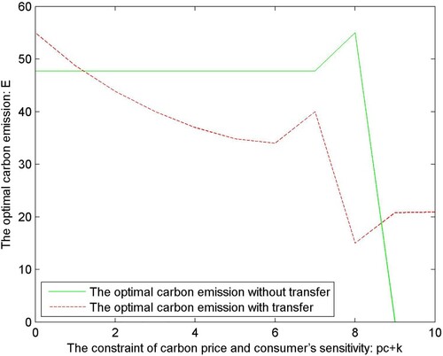
To a certain extent, the trend of lines in Figure 4 shows that the carbon price and the enhancement of consumers’ environmental awareness will promote enterprises to reduce production emissions and thus reduce carbon emissions. However, when the market limits carbon emissions too high, the product is no longer in line with the market requirements. In order to avoid the loss of their own interests, manufacturers will take measures to reduce or even stop production. At this time, the carbon emissions will gradually rise after the input of carbon emission transfer-related technologies.

For Theorem 4.3, we select $a=600,c=200,k=2,p_c=4,E_0=55,\text{β}=0.7$, t is taken as the explanatory variable, and the optimal carbon emission is the explained variable, where the value range of t is (0–20). Figure 5 shows the optimal carbon emissions before and after transfer as the cost coefficient increases, as shown in Figure 5.

Figure 5. The relationship between the optimal carbon emission and the cost coefficient of manufactures for unit emissions treatment.

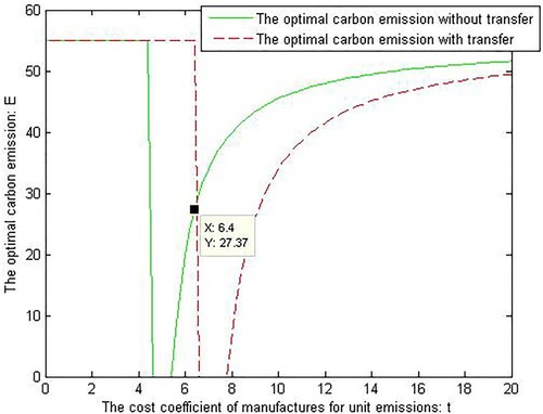
At this point $p_c+k=4<(a-c)/E_0=7.27$, and it can be seen from Figure 5 that $t\ge (p_c+k{)}^2/8\text{β}=7.5$, the carbon emission after transfer is smaller than that before transfer, so the manufacturer should choose to transfer part of carbon emission to the retailer.

As can be seen from the above picture, when carbon price and consumer environmental awareness constraint are within a certain range, carbon emission transfer will reduce the carbon emission of products. The higher the cost of emission reduction is, the carbon emission transfer is also beneficial to reduce the carbon emission of the product.

For Theorem 4.4, we select $a=600,c=200,t=10,k=2,p_c=4,E_0=55$.

In order to make $d{E}_{d\text{β}}^{\ast }$ takes valid value, the range of $\text{β}$ should be 0.55–1. The relationship between the variables and proportion undertaken by the manufacturer is shown in Figures 6–9.

Figure 6. The relationship between the optimal carbon emission and the proportion undertaken by the manufacturer.

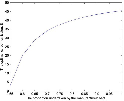
Figure 7. The relationship between the optimal wholesale price and the proportion undertaken by the manufacturer.

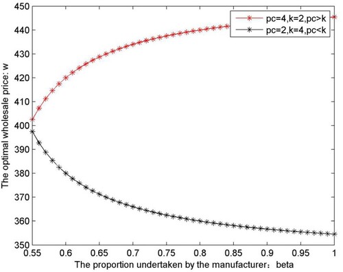
Figure 8. The relationship between the optimal demand and the proportion undertaken by the manufacturer.

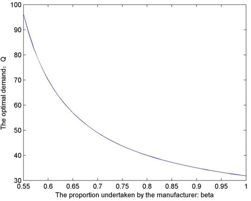
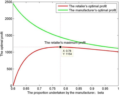
Figure 9. The relationship between the optimal profits and the proportion undertaken by the manufacturer.

The correctness of Theorem 4.4 (1) is proved from Figure 6, that the optimal emission $E_{d\text{β}}^{\ast }$ is increasing with the increase in $\text{β}$.

It can be seen that the values of $k$ and $p_c$ on the red line are 2 and 4. At this time, $k<p_c$, and the optimal wholesale price increases $w_{d\text{β}}^{\ast }$ with the increase in $\text{β}$. The values of k and p_c of the black line are 4 and 2. At this time, $k>p_c,w_{d\text{β}}^{\ast }$, decreases with the increase in $\text{β}$. So Theorem 4.4 (2) is verified to be correct. Then, it continues to verify the correctness of Theorem 4.4 (3).

Next, we continue to verify the correctness of Theorem 4.4 (3).

It can be seen that the optional demand $Q_{d\text{β}}^{\ast }$ decreases with the increase in $\text{β}$, and the correctness of Theorem 4.4 (3) is verified. Then, it continues to verify the correctness of Theorems 4.4 (4) and 4.4 (5).

Where $k=2,p_c=4,t=10$, in order to make $\prod _r^{d\text{β}\ast }\left(p\right)$ take valid value, the range of $\text{β}$ should be 0.6–1. As the red line represents the best profit trend for the retailer, we can know that the retailer's optimal benefit is 1154, and the corresponding value of $\text{β}$is 0.78. The left part of the dotted line is represented as $1-\text{β}>(p_c+k{)}^2/16t$, in which the optimal profit of the retailer $\prod _r^{d\text{β}\ast }\left(p\right)$ increases with the increases in $\text{β}$. While the right part of the dotted line is represented as $1-\text{β}<(p_c+k{)}^2/16t$, where $\prod _r^{d\text{β}\ast }\left(p\right)$ decreases with the increase in $\text{β}$. The green line represents the manufacturer, and we can see that the optimal profit of the manufacturer $\prod _m^{d\text{β}\ast }(w,E)$ decreases with the increase in $\text{β}$, so we use the actual data to prove the correctness of Theorem 4.3 and Theorem 4.4.

6. Conclusion and management significance

6.1. Conclusion

Under the carbon ‘Cap and Trade’ mechanism, manufacturers are facing dual pressure of emission reduction from the government and the market. But the manufacturer makes emission reduction decision mainly based on the maximization of enterprise income. If manufacturers can obtain carbon trading income and market’s favour by coordinating emission reduction transfer through supply chain, they will definitely take emission reduction transfer as an important factor in decision-making. Facing the consumers who are sensitive to the environment, retailers can get ‘free riding’ benefits through price premium, so as to actively promote manufacturers to reduce product emissions. When manufacturers transfer emission reduction tasks, retailers have the motivation to help manufacturers reduce emissions.

This paper establishes a two-stage game model between the retailer and the manufacturer, and analyses the decision-making strategies of the retailer in participating in the emission reduction process, which are constrained by carbon price and consumer environmental awareness under decentralized and centralized decisions. The specific conclusions are as follows.

(1) There is a threshold $(a-c)/E_0$ for dual constraints of carbon price and consumer environmental awareness. With the deepening of the manufacturer's emission reduction process, the input of emission reduction is increasing. If dual constraints continue to increase, the cost of the manufacturer's emission reduction input is less than the benefit of emission reduction, and the manufacturer lacks the motivation of emission reduction input. On the contrary, for the manufacturers who have just entered the ‘Cap and Trade’, the increasing constraints of both will promote manufacturers to invest in emission reduction.

(2) In the decentralized decision, when the manufacturer transfers the emission reduction task, the manufacturer's emission reduction cost $t$ corresponding to the threshold value $(a-c)/E_0$ becomes larger. That is because when the manufacturer has fewer emission reduction tasks, the emission reduction funds will be invested in fewer emission reduction tasks, the input of emission reduction tasks of per unit will increase, and the research and development of emission reduction technologies will be more deeper. The conditions for the manufacture to transfer emission reduction tasks are determined by the constraints of carbon price and consumer environmental awareness $p_c+k$, the proportion of emission reduction tasks undertaken by the manufacturer $\text{β}$ and the cost of emission reduction by the manufacturer $t$.

(3) For the manufacturer, the optimal emission reduction will increase with the increase in emission reduction tasks under the decentralized decision, but their profits will decrease accordingly. When the carbon price is high, if the manufacturer undertakes more emission reduction tasks, the manufacturer will make a strategy to increase the wholesale price. When the carbon price is low, if the manufacturer undertakes the higher emission reduction task, the manufacturer will make the strategy to decrease the wholesale price.

For the retailer, as the proportion undertaken by the retailer is $\alpha <(p_c+k{)}^2/16t$, the profit of retailers increases with the increase in $\text{β}$. When $\alpha >(p_c+k{)}^2/16t$; as the profit of the retailer decreases with the increase in $\text{β}$. Thus, the retailer can get the maximum profit, when it is $\alpha =(p_c+k{)}^2/16t$,

(4) In the decentralized decision, the emission reduction cost of the manufacturer $t$ corresponding to the threshold increases. This indicates that whether the manufacturer choose to transfer the emission task mainly depends on the impact of their behaviour on the income of the whole supply chain, as the more concentrated in manufacturer’ input in emission reduction is, the higher cost of per unit task is. The manufacturer and the retailer will form a group to share the profits from reducing emissions equally. When the manufacturer's emission reduction cost is higher than the retailer's, the manufacturer should increase the transfer proportion to make the retailer undertake more emission reduction tasks. When the retailer's emission reduction cost is higher than the manufacturer's, the manufacturer will undertake more emission reduction tasks.

6.2. Management significance

This paper studies the mechanism of carbon emission reduction that the retailer participates in under the ‘cap and trade’ system, analyses the formulation methods of emission reduction task under different decisions and provides important management significance for supply chain coordinators and carbon policy makers.

From the perspective of supply chain entities, the transfer of emission reduction tasks by the manufacturer is helpful for it to complete emission reduction plans, so as to obtain more benefits through ‘quota and trade’. The retailer can get ‘free riding’ benefits in the process of emission reduction, so it also has the willingness to reduce emissions. If the whole supply chain reduces emissions together, they can reduce more emissions and achieve a better emission reduction effect. Therefore, in order to achieve better effect in emission reduction and obtain more profits, the manufacturer and the retailer should build a collaborative supply chain to make consistent decisions. As the supply chain is unable to achieve synergy, we can also achieve the best decision for both sides in the game process. For the manufacturer, it can make the optimal wholesale price and the policy of emission reduction transfer according to the constraints of carbon price and consumer environmental awareness, and ultimately achieve the maximum revenue. For the retailer, it should determine the proportion of emission reduction according to its own income. At the same time, the retailer can set reasonable retail price to obtain price premium through consumer environmental awareness.

Since there is a threshold value $(a-c)/E_0$ of carbon price and consumer environmental awareness, and the threshold has different impacts on enterprises that have invested in emission reduction and those who have not, policy makers should formulate differentiated policies to promote supply chain entities to reduce carbon emissions. Policy makers should set the ‘ceiling’ of carbon price for enterprises that have already invested in emission reduction, thereby protecting their incentive to do so. For enterprises that do not invest in emission reduction, a carbon price ‘floor’ should be set to promote enterprises to invest in emission reduction (Wood & Frank, 2011). Manufacturers can realize ‘green washing’ by transferring emission reduction tasks, and consider establishing carbon disclosure policies to promote the development of low-carbon supply chain and realize the overall emission reduction of supply chain (Eun-Hee & Thomas, 2011).

Disclosure statement

No potential conflict of interest was reported by the author(s).

Additional information

Funding

The authors are grateful for the financial support provided by Humanities and Social Sciences Research Project of Chongqing Municipal Education Commission [grant number 20SKGH092] and Chongqing Municipal Education Commission Science and Technology Research Project [grant number KJZD-K202200707].

Appendix

Proof

Proof of Theorem 4.1

From Assumption 3.2 and Assumption 3.4, we can know: (A1) $\begin{array}{rl}Q& =a-p-kE\end{array}$(A1) (A2) $\begin{array}{rl}{C}_c& =t(E-E_0{)}^2\end{array}$(A2) The benefit function of the retailer and the benefit function of manufacturer under decentralized decision without transfer are as follows: (A3) $\begin{array}{rl}\prod _r^d\left(p\right)& =(p-w)Q=(p-w)(a-p-kE)\end{array}$(A3) (A4) $\begin{array}{rl}\prod _m(w,E)& =(w-c)Q-t(E-E_0{)}^2\\ & -p_c(EQ-E_{cap})s.t.0\le E\le E_0\end{array}$(A4) And now we have to take the derivative of (A3) and (A4): $\begin{array}{rl}\frac{d\prod _r^d\left(p\right)}{dp}& =\frac{d\left(\right(p-w\left)\right(a-p-kE\left)\right)}{dp}\\ & =-2p+w+a-kE\end{array}$If we make $\frac{d\prod _r^d\left(p\right)}{dp}=0$, we can get the values of $p$ and $Q$ as follows: $\begin{array}{rl}p& =\frac{a+w-kE}{2},Q=\frac{a-w-kE}{2},\\ \frac{\mathrm{\partial }\prod _m^d(w,E)}{\mathrm{\partial }w}& =\frac{\mathrm{\partial }\left(\right(w-c)Q-t{(E-E_0)}^2-p_c(EQ-E_{cap}\left)\right)}{\mathrm{\partial }w}\\ & =\frac{\begin{array}{c}\mathrm{\partial }\left(\right(w-c)\ast {\displaystyle \frac{a-w-kE}{2}}-t{(E-E_0)}^2\\ -p_c(E\ast {\displaystyle \frac{a-w-kE}{2}}-E_{cap}))\end{array}}{\mathrm{\partial }w}\\ & =-w+\frac{a-kE+c}{2}+\frac{p_{c}E}{2}.\end{array}$If we make $\frac{\mathrm{\partial }\prod _m^d(w,E)}{\mathrm{\partial }w}=0$, we can get the values of $w$ as follows: $\begin{array}{rl}w& =\frac{a+c+p_{c}E-kE}{2}\\ \frac{\mathrm{\partial }\prod _m^d(w,E)}{\mathrm{\partial }E}& =\frac{\mathrm{\partial }(wQ-cQ-t{(E-E_0)}^2-p_c(EQ-E_{cap}\left)\right)}{\mathrm{\partial }E}\\ & =\frac{\begin{array}{c}\mathrm{\partial }\left(\right(w-c)\ast {\displaystyle \frac{a-w-kE}{2}}-t{(E-E_0)}^2\\ -p_c(E\ast {\displaystyle \frac{a-w-kE}{2}}-E_{cap}))\end{array}}{\mathrm{\partial }E}\\ & =-\frac{k(w-c)}{2}+2t{E}_0-2tE-\frac{p_c(a-w)}{2}+p_{c}kE.\end{array}$If we make $\frac{\mathrm{\partial }\prod _m^d(w,E)}{\mathrm{\partial }E}=0$, we can get the values of $E$ as follows: $E=\frac{p_c(a-w)+k(w-c)-4t{E}_0}{2(p_{c}k-2t)}$If we substitute the value of $w=\frac{a+c+p_{c}E-kE}{2}$ into $E=\frac{p_c(a-w)+k(w-c)-4t{E}_0}{2(p_{c}k-2t)}$, we can get the equation as follows: $\begin{array}{l}((p_c+k{)}^2-8t)E_d^{\ast }=(a-c)(p_c+k)-8t{E}_0\\ (p_c+k{)}^2{E}_d^{\ast }-(a-c)(p_c+k)=8t{E}_d^{\ast }-8t{E}_0\end{array}$Then, we get the optimal carbon emission under decentralized decision without transfer as follows: $E_d^{\ast }=\frac{8t{E}_0-(a-c)(p_c+k)}{8t-{(p_c+k)}^2}$And $E_d^{\ast }-E_0=\frac{{(p_c+k)}^2{E}_0-(a-c)(p_c+k)}{8t-(p_c+k)}$

1. If we set $\frac{{(p_c+k)}^2{E}_0-(a-c)(p_c+k)}{8t-(p_c+k)}\ge 0$, we can get two inequalities as follows: $\begin{array}{r}\{\begin{array}{l}{\displaystyle \frac{{(p_c+k)}^2{E}_0-(a-c)(p_c+k)}{8t-(p_c+k)}}\ge 0\\ {\displaystyle \frac{8t{E}_0-(a-c)(p_c+k)}{8t-{(p_c+k)}^2}}\ge 0\end{array}\end{array}$

We can write the above two inequalities as follows: and to solve the inequality group: $\begin{array}{rl}& \{\begin{array}{l}(p_c+k{)}^2\ge {\displaystyle \frac{(a-c)}{E_0}}\\ t>{\displaystyle \frac{{(p_c+k)}^2}{8}}\end{array}\text{and}\\ & \{\begin{array}{l}(p_c+k{)}^2\le {\displaystyle \frac{(a-c)}{E_0}}\\ t<{\displaystyle \frac{{(p_c+k)}^2}{8}}\end{array}\end{array}$When the above inequality is satisfied, we have $E_d^{\ast }\ge E_0$.

Because we all know $0\le E_d^{\ast }\le E_0$, we can get the equation $E_d^{\ast }=E_0$.

1. If we set ${\displaystyle \frac{{(p_c+k)}^2{E}_0-(a-c)(p_c+k)}{8t-(p_c+k)}}<0$, we can get two inequalities as follows: $\begin{array}{r}\{\begin{array}{l}{\displaystyle \frac{{(p_c+k)}^2{E}_0-(a-c)(p_c+k)}{8t-(p_c+k)}}<0\\ {\displaystyle \frac{8t{E}_0-(a-c)(p_c+k)}{8t-{(p_c+k)}^2}}\ge 0\end{array}\end{array}$

We can write the above two inequalities as follows: $\begin{array}{rl}& \{\begin{array}{l}(p_c+k{)}^2{E}_0-(a-c)(p_c+k)>0\\ 8t-(p_c+k)<0\\ 8t{E}_0-(a-c)(p_c+k)\le 0\end{array}\text{and}\\ & \{\begin{array}{l}(p_c+k{)}^2{E}_0-(a-c)(p_c+k)<0\\ 8t-(p_c+k)>0\\ 8t{E}_0-(a-c)(p_c+k)\ge 0\end{array}\end{array}$To solve the inequality group: $\begin{array}{rl}& \{\begin{array}{l}(p_c+k{)}^2>{\displaystyle \frac{(a-c)}{E_0}}\\ t<{\displaystyle \frac{{(p_c+k)}^2}{8}}\end{array}\text{and}\\ & \{\begin{array}{l}(p_c+k{)}^2<{\displaystyle \frac{(a-c)}{E_0}}\\ t>{\displaystyle \frac{{(p_c+k)}^2}{8}}\end{array}\end{array}$When the above inequality is satisfied, we have $0<E_d^{\ast }<E_0$.

Therefore, we can get the equation $E_d^{\ast }={\displaystyle \frac{8t{E}_0-(a-c)(p_c+k)}{8t-{(p_c+k)}^2}}$.

1. If we set ${\displaystyle \frac{8t{E}_0-(a-c)(p_c+k)}{8t-{(p_c+k)}^2}}\le 0$, we can get two inequalities as follows: $\begin{array}{r}\{\begin{array}{l}{\displaystyle \frac{{(p_c+k)}^2{E}_0-(a-c)(p_c+k)}{8t-(p_c+k)}}<0\\ {\displaystyle \frac{8t{E}_0-(a-c)(p_c+k)}{8t-{(p_c+k)}^2}}\le 0\end{array}\end{array}$

We can write the above two inequalities as follows: $\begin{array}{rl}& \{\begin{array}{l}(p_c+k{)}^2{E}_0-(a-c)(p_c+k)\ge 0\\ 8t-(p_c+k)<0\end{array}\text{and}\\ & \{\begin{array}{l}(p_c+k{)}^2{E}_0-(a-c)(p_c+k)\le 0\\ 8t-(p_c+k)>0\end{array}\end{array}$To solve the inequality group: $\begin{array}{rl}& \{\begin{array}{l}(p_c+k{)}^2>{\displaystyle \frac{(a-c)}{E_0}}\\ {\displaystyle \frac{(a-c)(p_c+k)}{8E_0}}>t\ge {\displaystyle \frac{{(p_c+k)}^2}{8}}\end{array}\text{and}\\ & \{\begin{array}{l}(p_c+k{)}^2<{\displaystyle \frac{(a-c)}{E_0}}\\ {\displaystyle \frac{(a-c)(p_c+k)}{8E_0}}\ge t>{\displaystyle \frac{{(p_c+k)}^2}{8}}\end{array}\end{array}$When the above inequality is satisfied, we have $E_d^{\ast }\le 0$.

Because we all know $0\le E_d^{\ast }\le E_0$, we can get the equation $E_d^{\ast }=0$.

Proof

Proof of Theorem 4.2

The benefit function of the retailer and the benefit function of manufacturer under decentralized decision with transfer are as follows: (A5) $\begin{array}{rl}\prod _r^{d\text{β}}\left(p\right)& =(p-w)Q-t(1-\text{β})(E_0-E{)}^2\end{array}$(A5) (A6) $\begin{array}{rl}\prod _m^{d\text{β}}(w,E)& =(w-c)Q-t\text{β}(E_0-E{)}^2\\ & -p_c(EQ-E_{cap})s.t.0\le E\le E_0\end{array}$(A6) And now we have to take the derivative of (A5) and (A6): $\begin{array}{rl}{\displaystyle \frac{d\prod _r^{d\text{β}}\left(p\right)}{dp}}& ={\displaystyle \frac{d\left(\right(p-w\left)\right(a-p-kE)-t(1-\text{β}\left){(E-E_0)}^2\right)}{dp}}\\ & =-2p+w+a-kE\end{array}$If we make ${\displaystyle \frac{d\prod _r^{d\text{β}}\left(p\right)}{dp}}=0$, we can get the values of $p,Q$ as follows: $\begin{array}{rl}p& ={\displaystyle \frac{a+w-kE}{2}},Q={\displaystyle \frac{a-w-kE}{2}}\\ {\displaystyle \frac{\mathrm{\partial }\prod _m^{d\text{β}}(w,E)}{\mathrm{\partial }w}}& ={\displaystyle \frac{\mathrm{\partial }\left(\right(w-c)Q-t\text{β}{(E-E_0)}^2-p_c(EQ-E_{cap}\left)\right)}{\mathrm{\partial }w}}\\ & =\frac{\begin{array}{c}\mathrm{\partial }\left(\right(w-c)\ast {\displaystyle \frac{a-w-kE}{2}}-t\text{β}{(E-E_0)}^2\\ -p_c(E\ast {\displaystyle \frac{a-w-kE}{2}}-E_{cap}))\end{array}}{\mathrm{\partial }w}\\ & =-w+{\displaystyle \frac{a-kE+c}{2}}+{\displaystyle \frac{p_{c}E}{2}}\end{array}$If we make ${\displaystyle \frac{\mathrm{\partial }\prod _m^d(w,E)}{\mathrm{\partial }w}}=0$, we can get the values of $w$ as follows: $\begin{array}{rl}w& ={\displaystyle \frac{a+c+p_{c}E-kE}{2}}\\ {\displaystyle \frac{\mathrm{\partial }\prod _m^d(w,E)}{\mathrm{\partial }E}}& ={\displaystyle \frac{\mathrm{\partial }(wQ-cQ-t\text{β}{(E-E_0)}^2-p_c(EQ-E_{cap}\left)\right)}{\mathrm{\partial }E}}\\ & =\frac{\begin{array}{c}\mathrm{\partial }\left(\right(w-c)\ast {\displaystyle \frac{a-w-kE}{2}}-t\text{β}{(E-E_0)}^2\\ -p_c(E\ast {\displaystyle \frac{a-w-kE}{2}}-E_{cap}))\end{array}}{\mathrm{\partial }E}\\ & =-{\displaystyle \frac{k(w-c)}{2}}+2t\text{β}{E}_0\\ & -2t\text{β}E-{\displaystyle \frac{p_c(a-w)}{2}}+p_{c}kE\end{array}$If we make ${\displaystyle \frac{\mathrm{\partial }\prod _m^d(w,E)}{\mathrm{\partial }E}}=0$, we can get the values of $E$ as follows: $E={\displaystyle \frac{p_c(a-w)+k(w-c)-4t\text{β}{E}_0}{2(p_{c}k-2t\text{β})}}$If we substitute the value of $w={\displaystyle \frac{a+c+p_{c}E-kE}{2}}$ into $E={\displaystyle \frac{p_c(a-w)+k(w-c)-4t\text{β}{E}_0}{2(p_{c}k-2t\text{β})}}$, we can get the equation as follows: $((p_c+k{)}^2-8t\text{β})E_d^{\ast }=(a-c)(p_c+k)-8t\text{β}{E}_0$Then, we get the optimal carbon emission under decentralized decision with transfer as follows: $E_{d\text{β}}^{\ast }={\displaystyle \frac{8t\text{β}{E}_0-(a-c)(p_c+k)}{{8t\text{β}-(p_c+k)}^2}}$

And $E_d^{\ast }-E_0={\displaystyle \frac{{(p_c+k)}^2{E}_0-(a-c)(p_c+k)}{8t\text{β}-(p_c+k)}}$

1. If we set ${\displaystyle \frac{{(p_c+k)}^2{E}_0-(a-c)(p_c+k)}{8t\text{β}-(p_c+k)}}\ge 0$, we can get two inequalities as follows: $\begin{array}{r}\{\begin{array}{l}{\displaystyle \frac{{(p_c+k)}^2{E}_0-(a-c)(p_c+k)}{8t\text{β}-(p_c+k)}}\ge 0\\ {\displaystyle \frac{8t\text{β}{E}_0-(a-c)(p_c+k)}{8t\text{β}-{(p_c+k)}^2}}\ge 0\end{array}\end{array}$

We can write the above two inequalities as follows: $\begin{array}{rl}& \{\begin{array}{l}(p_c+k{)}^2{E}_0-(a-c)(p_c+k)\ge 0\\ 8t\text{β}-(p_c+k)>0\\ 8t\text{β}{E}_0-(a-c)(p_c+k)\ge 0\end{array}\text{and}\\ & \{\begin{array}{l}(p_c+k{)}^2{E}_0-(a-c)(p_c+k)\le 0\\ 8t\text{β}-(p_c+k)<0\\ 8t\text{β}{E}_0-(a-c)(p_c+k)\le 0\end{array}\end{array}$To solve the inequality group: $\begin{array}{rl}& \{\begin{array}{l}(p_c+k{)}^2\ge {\displaystyle \frac{(a-c)}{E_0}}\\ t>{\displaystyle \frac{{(p_c+k)}^2}{8\text{β}}}\end{array}\text{and}\\ & \{\begin{array}{l}(p_c+k{)}^2\le {\displaystyle \frac{(a-c)}{E_0}}\\ t<{\displaystyle \frac{{(p_c+k)}^2}{8\text{β}}}\end{array}\end{array}$When the above inequality is satisfied, we have $E_{d\text{β}}^{\ast }\ge E_0$.

Because we all know $0\le E_{d\text{β}}^{\ast }\le E_0$, we can get the equation $E_{d\text{β}}^{\ast }=E_0$.

1. If we set ${\displaystyle \frac{{(p_c+k)}^2{E}_0-(a-c)(p_c+k)}{8t\text{β}-(p_c+k)}}<0$, we can get two inequalities as follows: $\begin{array}{r}\{\begin{array}{l}{\displaystyle \frac{{(p_c+k)}^2{E}_0-(a-c)(p_c+k)}{8t\text{β}-(p_c+k)}}<0\\ {\displaystyle \frac{8t\text{β}{E}_0-(a-c)(p_c+k)}{8t\text{β}-{(p_c+k)}^2}}\ge 0\end{array}\end{array}$

We can write the above two inequalities as follows: $\begin{array}{rl}& \{\begin{array}{l}(p_c+k{)}^2{E}_0-(a-c)(p_c+k)>0\\ 8t\text{β}-(p_c+k)<0\\ 8t\text{β}{E}_0-(a-c)(p_c+k)\le 0\end{array}\text{and}\\ & \{\begin{array}{l}(p_c+k{)}^2{E}_0-(a-c)(p_c+k)<0\\ 8t\text{β}-(p_c+k)>0\\ 8t\text{β}{E}_0-(a-c)(p_c+k)\ge 0\end{array}\end{array}$To solve the inequality group: $\begin{array}{rl}& \{\begin{array}{l}(p_c+k{)}^2>{\displaystyle \frac{(a-c)}{E_0}}\\ t<{\displaystyle \frac{{(p_c+k)}^2}{8\text{β}{E}_0}}\end{array}\text{and}\\ & \{\begin{array}{l}(p_c+k{)}^2<{\displaystyle \frac{(a-c)}{E_0}}\\ t>{\displaystyle \frac{{(p_c+k)}^2}{8\text{β}{E}_0}}\end{array}\end{array}$When the above inequality is satisfied, we have $0<E_{d\text{β}}^{\ast }<E_0$.

Therefore, we can get the equation $E_{d\text{β}}^{\ast }={\displaystyle \frac{8t\text{β}{E}_0-(a-c)(p_c+k)}{8t\text{β}-{(p_c+k)}^2}}$.

1. If we set ${\displaystyle \frac{8t\text{β}{E}_0-(a-c)(p_c+k)}{8t\text{β}-{(p_c+k)}^2}}\le 0$, we can get two inequalities as follows: $\begin{array}{r}\{\begin{array}{l}{\displaystyle \frac{{(p_c+k)}^2{E}_0-(a-c)(p_c+k)}{8t\text{β}-(p_c+k)}}<0\\ {\displaystyle \frac{8t\text{β}{E}_0-(a-c)(p_c+k)}{8t\text{β}-{(p_c+k)}^2}}\le 0\end{array}\end{array}$

We can write the above two inequalities as follows: $\begin{array}{rl}& \{\begin{array}{l}8t\text{β}{E}_0-(a-c)(p_c+k)\ge 0\\ 8t\text{β}-(p_c+k{)}^2<0\end{array}\text{and}\\ & \{\begin{array}{l}8t\text{β}{E}_0-(a-c)(p_c+k)\le 0\\ 8t\text{β}-(p_c+k{)}^2>0\end{array}\end{array}$To solve the inequality group: $\begin{array}{rl}& \{\begin{array}{l}(p_c+k{)}^2>{\displaystyle \frac{(a-c)}{E_0}}\\ {\displaystyle \frac{{(p_c+k)}^2}{8\text{β}}}>t\ge {\displaystyle \frac{(a-c)(p_c+k)}{8\text{β}{E}_0}}\end{array}\\ & \text{and}\{\begin{array}{l}(p_c+k{)}^2<{\displaystyle \frac{(a-c)}{E_0}}\\ {\displaystyle \frac{{(p_c+k)}^2}{8\text{β}}}\ge t>{\displaystyle \frac{(a-c)(p_c+k)}{8\text{β}{E}_0}}\end{array}\end{array}$When the above inequality is satisfied, we have $E_{d\text{β}}^{\ast }\le 0$.

Because we all know $0\le E_{d\text{β}}^{\ast }\le E_0$, we can get the equation $E_{d\text{β}}^{\ast }=0$.

Proof

Proof of Theorem 4.3

This question can be divided into the following cases to prove:

Case 1: $p_c+k\ge {\displaystyle \frac{a-c}{E_0}}$

Given that $\text{β}$ is less than 1, it can be divided into two cases: $(p_c+k)\text{β}\ge {\displaystyle \frac{a-c}{E_0}}$ and $(p_c+k)\text{β}\le {\displaystyle \frac{a-c}{E_0}}$.

1. when $(p_c+k)\text{β}\le {\displaystyle \frac{a-c}{E_0}}$, the following inequality is true: $\begin{array}{rl}{\displaystyle \frac{(a-c)(p_c+k)}{8E_0}}& <{\displaystyle \frac{{(p_c+k)}^2}{8}}\\ & <{\displaystyle \frac{(a-c)(p_c+k)}{8\text{β}{E}_0}}<{\displaystyle \frac{{(p_c+k)}^2}{8\text{β}}}\end{array}$

According to Theorems 4.1 and 4.2, we can draw the following conclusions:

1. When $t<{\displaystyle \frac{(a-c)(p_c+k)}{8E_0}}$, the following equations are true: $\begin{array}{rl}{E}_{d\text{β}}^{\ast }& ={\displaystyle \frac{8t\text{β}{E}_0-(a-c)(p_c+k)}{8t\text{β}-{(p_c+k)}^2}}\text{and}\\ E_d^{\ast }& ={\displaystyle \frac{8t{E}_0-(a-c)(p_c+k)}{8t-{(p_c+k)}^2}}\end{array}$

And $E_{d\text{β}}^{\ast }-E_d^{\ast }={\displaystyle \frac{8t(1-\text{β})(p_c+k)\left(\right(p_c+k)E_0-(a-c\left)\right)}{(8t\text{β}-{(p_c+k)}^2)(8t-{(p_c+k)}^2)}}\ge 0$. Therefore, we have $E_{d\text{β}}^{\ast }\ge E_d^{\ast }$.

• (ii) When ${\displaystyle \frac{(a-c)(p_c+k)}{8E_0}}\le t<{\displaystyle \frac{{(p_c+k)}^2}{8}}$, the following equations are true: $E_{d\text{β}}^{\ast }={\displaystyle \frac{8t\text{β}{E}_0-(a-c)(p_c+k)}{8t\text{β}-{(p_c+k)}^2}}\text{and}{E}_d^{\ast }=0$

And $E_{d\text{β}}^{\ast }-E_d^{\ast }={\displaystyle \frac{8t\text{β}{E}_0-(a-c)(p_c+k)}{8t\text{β}-{(p_c+k)}^2}}\ge 0$. Therefore, we have $E_{d\text{β}}^{\ast }\ge E_d^{\ast }$.

• (iii) When ${\displaystyle \frac{{(p_c+k)}^2}{8}}\le t<{\displaystyle \frac{(a-c)(p_c+k)}{8\text{β}{E}_0}}$, the following equations are true: $E_{d\text{β}}^{\ast }={\displaystyle \frac{8t\text{β}{E}_0-(a-c)(p_c+k)}{8t\text{β}-{(p_c+k)}^2}}\text{and}{E}_d^{\ast }=E_0$

And $E_{d\text{β}}^{\ast }-E_d^{\ast }={\displaystyle \frac{{(p_c+k)}^2{E}_0-(a-c)(p_c+k)}{8t\text{β}-{(p_c+k)}^2}}\ge 0$.

Therefore, we have $E_{d\text{β}}^{\ast }\le E_d^{\ast }$.

• (iv) When ${\displaystyle \frac{(a-c)(p_c+k)}{8\text{β}{E}_0}}\le t<{\displaystyle \frac{{(p_c+k)}^2}{8\text{β}}}$, the following equations are true: $E_{d\text{β}}^{\ast }=0\text{and}{E}_d^{\ast }=E_0$

And $E_{d\text{β}}^{\ast }-E_d^{\ast }=-E_0<0$.

Therefore, we have $E_{d\text{β}}^{\ast }\le E_d^{\ast }$.

1. When $t\ge {\displaystyle \frac{{(p_c+k)}^2}{8\text{β}}}$, the following equations are true: $E_{d\text{β}}^{\ast }=E_0\text{and}{E}_d^{\ast }=E_0$

Therefore, we have $E_{d\text{β}}^{\ast }=E_d^{\ast }$.

1. when $(p_c+k)\text{β}\ge {\displaystyle \frac{a-c}{E_0}}$, the following inequality is true: $\begin{array}{r}{\displaystyle \frac{(a-c)(p_c+k)}{8E_0}}\\ & <{\displaystyle \frac{(a-c)(p_c+k)}{8\text{β}{E}_0}}<{\displaystyle \frac{{(p_c+k)}^2}{8}}<{\displaystyle \frac{{(p_c+k)}^2}{8\text{β}}}\end{array}$

According to Theorems 4.1 and 4.2, we can draw the following conclusions:

1. When $t<{\displaystyle \frac{(a-c)(p_c+k)}{8E_0}}$, the following equations are true: $\begin{array}{rl}{E}_{d\text{β}}^{\ast }& ={\displaystyle \frac{8t\text{β}{E}_0-(a-c)(p_c+k)}{8t\text{β}-{(p_c+k)}^2}}\text{and}\\ E_d^{\ast }& ={\displaystyle \frac{8t{E}_0-(a-c)(p_c+k)}{8t-{(p_c+k)}^2}}\end{array}$

And $E_{d\text{β}}^{\ast }-E_d^{\ast }={\displaystyle \frac{8t(1-\text{β})(p_c+k)\left(\right(p_c+k)E_0-(a-c\left)\right)}{(8t\text{β}-{(p_c+k)}^2)(8t-{(p_c+k)}^2)}}\ge 0$. Therefore, we have $E_{d\text{β}}^{\ast }\ge E_d^{\ast }$.

• (ii) When ${\displaystyle \frac{(a-c)(p_c+k)}{8E_0}}\le t<{\displaystyle \frac{(a-c)(p_c+k)}{8\text{β}{E}_0}}$, the following equations are true: $E_{d\text{β}}^{\ast }={\displaystyle \frac{8t\text{β}{E}_0-(a-c)(p_c+k)}{8t\text{β}-{(p_c+k)}^2}}\text{and}{E}_d^{\ast }=0$

And $E_{d\text{β}}^{\ast }-E_d^{\ast }={\displaystyle \frac{8t\text{β}{E}_0-(a-c)(p_c+k)}{8t\text{β}-{(p_c+k)}^2}}\ge 0$. Therefore, we have $E_{d\text{β}}^{\ast }\ge E_d^{\ast }$.

• (iii) When ${\displaystyle \frac{(a-c)(p_c+k)}{8\text{β}{E}_0}}\le t<{\displaystyle \frac{{(p_c+k)}^2}{8}}$, the following equations are true: $E_{d\text{β}}^{\ast }=0\text{and}{E}_d^{\ast }=0$

Therefore, we have $E_{d\text{β}}^{\ast }=E_d^{\ast }$.

• (iv) When ${\displaystyle \frac{{(p_c+k)}^2}{8}}\le t<{\displaystyle \frac{{(p_c+k)}^2}{8\text{β}}}$, the following equations are true: $E_{d\text{β}}^{\ast }=0\text{and}{E}_d^{\ast }=E_0\text{and}{E}_{d\text{β}}^{\ast }-E_d^{\ast }=-E_0<0$

Therefore, we have $E_{d\text{β}}^{\ast }\le E_d^{\ast }$.

1. When $t\ge {\displaystyle \frac{{(p_c+k)}^2}{8\text{β}}}$, the following equations are true: $E_{d\text{β}}^{\ast }=E_0\text{and}{E}_d^{\ast }=E_0$

Therefore, we have $E_{d\text{β}}^{\ast }=E_d^{\ast }$.

Case 2: $p_c+k\le {\displaystyle \frac{a-c}{E_0}}$

Given that $\text{β}$ is less than 1, it can be divided into two cases: ${\displaystyle \frac{(p_c+k)}{\text{β}}}\le {\displaystyle \frac{a-c}{E_0}}$ and ${\displaystyle \frac{(p_c+k)}{\text{β}}}\ge {\displaystyle \frac{a-c}{E_0}}$.

1. when $(p_c+k)\text{β}\ge {\displaystyle \frac{a-c}{E_0}}$, the following inequality is true: $\begin{array}{rl}{\displaystyle \frac{{(p_c+k)}^2}{8}}& <{\displaystyle \frac{(a-c)(p_c+k)}{8E_0}}<{\displaystyle \frac{{(p_c+k)}^2}{8\text{β}}}\\ & <{\displaystyle \frac{(a-c)(p_c+k)}{8\text{β}{E}_0}}\end{array}$

According to Theorems 4.1 and 4.2, we can draw the following conclusions:

1. When $t<{\displaystyle \frac{{(p_c+k)}^2}{8}}$, the following equations are true: $E_{d\text{β}}^{\ast }=E_0\text{and}{E}_d^{\ast }=E_0$

Therefore, we have $E_{d\text{β}}^{\ast }=E_d^{\ast }$.

• (ii) When ${\displaystyle \frac{{(p_c+k)}^2}{8}}<t\le {\displaystyle \frac{(a-c)(p_c+k)}{8E_0}}$, the following equations are true: $E_{d\text{β}}^{\ast }=E_{0}and{E}_d^{\ast }=0$

And $E_{d\text{β}}^{\ast }-E_d^{\ast }=E_0\ge 0$. Therefore, we have $E_{d\text{β}}^{\ast }\ge E_d^{\ast }$.

• (iii) When ${\displaystyle \frac{(a-c)(p_c+k)}{8E_0}}<t\le {\displaystyle \frac{{(p_c+k)}^2}{8\text{β}}}$, the following equations are true: $E_{d\text{β}}^{\ast }=E_0$and $E_d^{\ast }={\displaystyle \frac{8t{E}_0-(a-c)(p_c+k)}{8t-{(p_c+k)}^2}}$.

And $E_{d\text{β}}^{\ast }-E_d^{\ast }={\displaystyle \frac{(a-c)(p_c+k)-{(p_c+k)}^2{E}_0}{8t-{(p_c+k)}^2}}\ge 0$. Therefore, we have $E_{d\text{β}}^{\ast }\ge E_d^{\ast }$.

• (iv) When ${\displaystyle \frac{{(p_c+k)}^2}{8\text{β}}}<t\le {\displaystyle \frac{(a-c)(p_c+k)}{8\text{β}{E}_0}}$, the following equations are true:

$E_{d\text{β}}^{\ast }=0$ and $E_d^{\ast }={\displaystyle \frac{8t{E}_0-(a-c)(p_c+k)}{8t-{(p_c+k)}^2}}$. And $E_{d\text{β}}^{\ast }-E_d^{\ast }=-{\displaystyle \frac{8t{E}_0-(a-c)(p_c+k)}{8t-{(p_c+k)}^2}}\le 0$. Therefore, we have $E_{d\text{β}}^{\ast }\le E_d^{\ast }$.

1. When $t>{\displaystyle \frac{(a-c)(p_c+k)}{8\text{β}{E}_0}}$, the following equations are true: $\begin{array}{rl}{E}_{d\text{β}}^{\ast }& ={\displaystyle \frac{8t\text{β}{E}_0-(a-c)(p_c+k)}{8t\text{β}-{(p_c+k)}^2}}\text{and}\\ E_d^{\ast }& ={\displaystyle \frac{8t{E}_0-(a-c)(p_c+k)}{8t-{(p_c+k)}^2}}\end{array}$

And $E_{d\text{β}}^{\ast }-E_d^{\ast }={\displaystyle \frac{8t(1-\text{β})(p_c+k)\left(\right(p_c+k)E_0-(a-c\left)\right)}{(8t\text{β}-{(p_c+k)}^2)(8t-{(p_c+k)}^2)}}\le 0$. Therefore, we have $E_{d\text{β}}^{\ast }\le E_d^{\ast }$.

1. when ${\displaystyle \frac{(p_c+k)}{\text{β}}}\le {\displaystyle \frac{a-c}{E_0}}$, the following inequality is true: $\begin{array}{rl}{\displaystyle \frac{{(p_c+k)}^2}{8}}& <{\displaystyle \frac{{(p_c+k)}^2}{8\text{β}}}<{\displaystyle \frac{(a-c)(p_c+k)}{8E_0}}\\ & <{\displaystyle \frac{(a-c)(p_c+k)}{8\text{β}{E}_0}}\end{array}$

According to Theorems 4.1 and 4.2, we can draw the following conclusions:

1. When $t<{\displaystyle \frac{{(p_c+k)}^2}{8}}$, the following equations are true: $E_{d\text{β}}^{\ast }=E_0\text{and}{E}_d^{\ast }=E_0$

Therefore, we have $E_{d\text{β}}^{\ast }=E_d^{\ast }$.

• (ii) When ${\displaystyle \frac{{(p_c+k)}^2}{8}}<t\le {\displaystyle \frac{{(p_c+k)}^2}{8\text{β}}}$, the following equations are true:

$E_{d\text{β}}^{\ast }=E_0$ and $E_d^{\ast }=0$. And $E_{d\text{β}}^{\ast }-E_d^{\ast }=E_0\ge 0$. Therefore, we have $E_{d\text{β}}^{\ast }\ge E_d^{\ast }$.

• (iii) When ${\displaystyle \frac{{(p_c+k)}^2}{8\text{β}}}<t\le {\displaystyle \frac{(a-c)(p_c+k)}{8E_0}}$, the following equations are true:

$E_{d\text{β}}^{\ast }=0$ and $E_d^{\ast }=0$. Therefore, we have $E_{d\text{β}}^{\ast }=E_d^{\ast }$.

• (iv) When ${\displaystyle \frac{(a-c)(p_c+k)}{8E_0}}<t\le {\displaystyle \frac{(a-c)(p_c+k)}{8\text{β}{E}_0}}$, the following equations are true: $E_{d\text{β}}^{\ast }=0\text{and}{E}_d^{\ast }={\displaystyle \frac{8t{E}_0-(a-c)(p_c+k)}{8t-{(p_c+k)}^2}}$

And $E_{d\text{β}}^{\ast }-E_d^{\ast }=-{\displaystyle \frac{8t{E}_0-(a-c)(p_c+k)}{8t-{(p_c+k)}^2}}\le 0$. Therefore, we have $E_{d\text{β}}^{\ast }\le E_d^{\ast }$.

1. When $t>{\displaystyle \frac{(a-c)(p_c+k)}{8\text{β}{E}_0}}$, the following equations are true: $\begin{array}{rl}{E}_{d\text{β}}^{\ast }& ={\displaystyle \frac{8t\text{β}{E}_0-(a-c)(p_c+k)}{8t\text{β}-{(p_c+k)}^2}}\text{and}\\ E_d^{\ast }& ={\displaystyle \frac{8t{E}_0-(a-c)(p_c+k)}{8t-{(p_c+k)}^2}}\end{array}$

And $E_{d\text{β}}^{\ast }-E_d^{\ast }={\displaystyle \frac{8t(1-\text{β})(p_c+k)\left(\right(p_c+k)E_0-(a-c\left)\right)}{(8t\text{β}-{(p_c+k)}^2)(8t-{(p_c+k)}^2)}}\le 0$. Therefore, we have $E_{d\text{β}}^{\ast }\le E_d^{\ast }$.

Proof

Proof of Theorem 4.4

Since the discussion of $E_{d\text{β}}^{\ast }$ in the case of $E_d^{\ast }=E_0$ and $E_d^{\ast }=0$ has no practical significance, so we only discuss the change of other variables with $\text{β}$ in the presence of $E_{d\text{β}}^{\ast }={\displaystyle \frac{8t\text{β}{E}_0-(a-c)(p_c+k)}{8t\text{β}-{(p_c+k)}^2}}\ne 0$.

And if other variables are to be studied to see whether they change with the increase in $\text{β}$, the premise is that the selected optimization decision is the transfer of emission reduction task, i.e. $E_{d\text{β}}^{\ast }\le E_d^{\ast }$. Here, we take $E_d^{\ast }={\displaystyle \frac{8t{E}_0-(a-c)(p_c+k)}{8t-{(p_c+k)}^2}}$, which is: $E_{d\text{β}}^{\ast }-E_d^{\ast }={\displaystyle \frac{8t(1-\text{β})(p_c+k)\left(\right(p_c+k)E_0-(a-c\left)\right)}{(8t\text{β}-{(p_c+k)}^2)(8t-{(p_c+k)}^2)}}\le 0$We can get (A7) from the above inequality: (7) $\begin{array}{r}(p_c+k)E_0-(a-c)\le 0\end{array}$(7)

1. And now we have to take the derivative of $E_{d\text{β}}^{\ast }$: $\begin{array}{rl}{\displaystyle \frac{d{E}_{d\text{β}}^{\ast }}{d\text{β}}}& ={\displaystyle \frac{\begin{array}{c}8t{E}_0(8t\text{β}-{(p_c+k)}^2)\\ -[8t{E}_0\text{β}-(a-c\left)\right(p_c+k\left)\right]8t\end{array}}{{(8t\text{β}-{(p_c+k)}^2)}^2}}\\ & ={\displaystyle \frac{\begin{array}{c}64t^2{E}_0\text{β}-8{(p_c+k)}^{2}t{E}_0-64t^2{E}_0\text{β}\\ +8t(a-c)(p_c+k)\end{array}}{{(8t\text{β}-{(p_c+k)}^2)}^2}}\\ & ={\displaystyle \frac{8t(p_c+k)[a-c-(p_c+k\left)E_0\right]}{{(8t\text{β}-{(p_c+k)}^2)}^2}}\end{array}$

From (A5) we can get this:${\displaystyle \frac{d{E}_{d\text{β}}^{\ast }}{d\text{β}}}\ge 0$

Therefore, we can know that the optimal emission $E_{d\text{β}}^{\ast }$ is increasing with $\text{β}$.

1. We work out the optimal wholesale price $w_{d\text{β}}^{\ast }$ as follows: $w_{d\text{β}}^{\ast }={\displaystyle \frac{(p_c+k)(p_{c}a+kc)+4t{E}_0\text{β}(k-p_c)-4t\text{β}(a+c)}{{(p_c+k)}^2-8t\text{β}}}$

And now we have to take the derivative of $w_{d\text{β}}^{\ast }$: $\begin{array}{rl}{\displaystyle \frac{d{w}_{d\text{β}}^{\ast }}{d\text{β}}}& ={\displaystyle \frac{\begin{array}{c}\left[4t{E}_0\right(k-p_c)-4t(a+c\left)\right][{(p_c+k)}^2-8t\text{β}]\\ +8t\left[\right(p_c+k\left)\right(p_{c}a+kc)+4t{E}_0\text{β}(k-p_c)-4t\text{β}(a+c\left)\right]\end{array}}{{({(p_c+k)}^2-8t\text{β})}^2}}\\ & ={\displaystyle \frac{4t(p_c+k)(k-p_c)\left[\right(p_c+k\left)E_0\text{ - }\right(a-c\left)\right]}{{({(p_c+k)}^2-8t\text{β})}^2}}\end{array}$From (A5) we can get conclusions as follows:

If $k<p_c$, there is ${\displaystyle \frac{d{w}_{d\text{β}}^{\ast }}{d\text{β}}}\ge 0$ and we can know that the optimal wholesale price $w_{d\text{β}}^{\ast }$ is increasing with $\text{β}$.

If $k>p_c$, there is ${\displaystyle \frac{d{w}_{d\text{β}}^{\ast }}{d\text{β}}}\le 0$ and we can know that the optimal wholesale price $w_{d\text{β}}^{\ast }$ is decreasing with $\text{β}$.

1. We work out the optimal wholesale price $Q_{d\text{β}}^{\ast }$ as follows: $Q_{d\text{β}}^{\ast }={\displaystyle \frac{2t\text{β}\left[\right(p_c+k)E_0-(a-c\left)\right]}{{(p_c+k)}^2-8t\text{β}}}$

And now we have to take the derivative of $Q_{d\text{β}}^{\ast }$: $\begin{array}{cc}{\displaystyle \frac{d{Q}_{d\text{β}}^{\ast }}{d\text{β}}}& ={\displaystyle \frac{\begin{array}{c}2t\left[\right(p_c+k)E_0-(a-c\left)\right][{(p_c+k)}^2-8t\text{β}]\\ +8t\left[2t\text{β}\right[(p_c+k)E_0-(a-c)]\end{array}}{{({(p_c+k)}^2-8t\text{β})}^2}}\\ & ={\displaystyle \frac{2t\left[\right(p_c+k)E_0-(a-c\left)\right]{(p_c+k)}^2}{{(8t\text{β}-{(p_c+k)}^2)}^2}}\end{array}$From (S5) we can get this: ${\displaystyle \frac{d{Q}_{d\text{β}}^{\ast }}{d\text{β}}}\le 0$.

Therefore, we can know that the optimal emission $Q_{d\text{β}}^{\ast }$ is decreasing with $\text{β}$.

1. We work out the manufacturer’s optimal profit $\prod _m^{d\text{β}\ast }(w,E)$ as follows: $\begin{array}{l}\prod _r^{d\text{β}\ast }\left(p\right)=(p^{\ast }-w^{\ast })Q^{\ast }-t(1-\text{β})(E_0-E^{\ast }{)}^2\\ ={\displaystyle \frac{{\left[\right(p_c+k)E_0-(a-c\left)\right]}^2[4t^2{\text{β}}^2-t(1-\text{β}\left){(p_c+k)}^2\right]}{{[8t\text{β}-{(p_c+k)}^2]}^2}}\end{array}$

And now we have to take the derivative of $\prod _r^{d\text{β}\ast }\left(p\right)$: $\begin{array}{rl}{\displaystyle \frac{d\prod _r^{d\text{β}\ast }\left(p\right)}{d\text{β}}}& ={\displaystyle \frac{\begin{array}{c}[8t^2\text{β}+t{(p_c+k)}^2]\\ {\left[\right(p_c+k)E_0-(a-c\left)\right]}^2]{(8t\text{β}-{(p_c+k)}^2)}^2\end{array}}{{({(p_c+k)}^2-8t\text{β})}^4}}\\ & -{\displaystyle \frac{\begin{array}{c}[4t^2{\text{β}}^2-t(1-\text{β}\left){(p_c+k)}^2\right]\\ {\left[\right(p_c+k)E_0-(a-c\left)\right]}^2\left]16t\right(8t\text{β}-{(p_c+k)}^2)\end{array}}{{({(p_c+k)}^2-8t\text{β})}^4}}\\ & ={\displaystyle \frac{\begin{array}{c}t{(p_c+k)}^2{\left[\right(p_c+k)E_0-(a-c\left)\right]}^2\\ \left[16\right(1-\text{β})t-{(p_c+k)}^2]\end{array}}{{(8t\text{β}-{(p_c+k)}^2)}^3}}\end{array}$From (A5) we can get conclusions as follows:

• If $1-\text{β}<{\displaystyle \frac{{(p_c+k)}^2}{16t}}$, there is ${\displaystyle \frac{d\prod _r^{d\text{β}\ast }\left(p\right)}{d\text{β}}}\ge 0$ and we can know that the retailer’s optimal profit $\prod _r^{d\text{β}\ast }\left(p\right)$ is decreasing with $\text{β}$.

• If $1-\text{β}>{\displaystyle \frac{{(p_c+k)}^2}{16t}}$, there is ${\displaystyle \frac{d\prod _r^{d\text{β}\ast }\left(p\right)}{d\text{β}}}\le 0$ and we can know that the retailer’s optimal profit $\prod _r^{d\text{β}\ast }\left(p\right)$ is increasing with $\text{β}$.

1. We work out the manufacturer’s optimal profit $\prod _m^{d\text{β}\ast }(w,E)$ as follows: $\begin{array}{rl}\prod _m^{d\text{β}\ast }(w,E)& =(w^{\ast }-c)Q^{\ast }-t\text{β}(E^{\ast }-E_0{)}^2-p_c(EQ-E_{cap})\\ & ={\displaystyle \frac{t\text{β}{\left[\right(p_c+k)E_0-(a-c\left)\right]}^2}{8t\text{β}-{(p_c+k)}^2}}\end{array}$

And now we have to take the derivative of $\prod _m^{d\text{β}\ast }(w,E)$: $\begin{array}{ll}{\displaystyle \frac{d\prod _m^{d\text{β}\ast }(w,E)}{d\text{β}}}& ={\displaystyle \frac{\begin{array}{c}t{\left[\right(p_c+k)E_0-(a-c\left)\right]}^2{[8t\text{β}-{(p_c+k)}^2]}^2\\ -8t^2\text{β}{\left[\right(p_c+k)E_0-(a-c\left)\right]}^2\end{array}}{{(8t\text{β}-{(p_c+k)}^2)}^2}}\\ & =-{\displaystyle \frac{t{(p_c+k)}^2{\left[\right(p_c+k)E_0-(a-c\left)\right]}^2}{{(8t\text{β}-{(p_c+k)}^2)}^2}}\end{array}$From (A5) we can get this: ${\displaystyle \frac{d\prod _m^{d\text{β}\ast }(w,E)}{d\text{β}}}\le 0$.

Therefore, we can know that the manufacturer’s optimal profit $\prod _m^{d\text{β}\ast }(w,E)$ is decreasing with $\text{β}$.

Proof

Proof of Theorem 4.5

The benefit function of the whole system under centralized decision is as follows: (A8) $\begin{array}{rl}& {\prod }_s^{}(p,E)\\ & =(p-c)Q-t(E_0-E{)}^2-p_c(EQ-E_{cap})..s.t.0\le E\le E_0\end{array}$(A8) And now we have to take the derivative of (A8): ${\displaystyle \frac{d\prod _s(p,E)}{dp}}=-2p+a+c-kE+p_{c}E$If we make ${\displaystyle \frac{d\prod _s^{}(p,E)}{dp}}=0$, we can get the values of $p$ as follows: $\begin{array}{rl}p& ={\displaystyle \frac{a+c+(p_c-k)E}{2}}{\displaystyle \frac{d\prod _s(p,E)}{dE}}=-k(p-c)\\ & +2t(E_0-E)-(a-p)p_c+2p_{c}kE\end{array}$If we make ${\displaystyle \frac{d\prod _s^{}(p,E)}{dE}}=0$, we can get the values of $E$ as follows: $E={\displaystyle \frac{k(p-c)+(a-p)p_c-2t{E}_0}{2(p_{c}k-t)}}$If we substitute the value of $p$ into $E$, we can get equation as follows: $4t{E}_0-(k+p_c)(a-c)=[4t-(p_c+k{)}^2]E_s^{\ast }$Then we get the optimal carbon emission under centralized decision as follows: $E_s^{\ast }={\displaystyle \frac{4t{E}_0-(p_c+k)(a-c)}{4t-{(p_c+k)}^2}}\ge \text{0}$And $E_s^{\ast }\text{ - }{E}_0={\displaystyle \frac{{(p_c+k)}^2{E}_0-(p_c+k)(a-c)}{4t-{(p_c+k)}^2}}$

1. If we set ${\displaystyle \frac{{(p_c+k)}^2{E}_0-(p_c+k)(a-c)}{4t-{(p_c+k)}^2}}\ge \text{0}$, we can get two inequalities as follows: $\{\begin{array}{l}{\displaystyle \frac{{(p_c+k)}^2{E}_0-(p_c+k)(a-c)}{4t-{(p_c+k)}^2}}\ge \text{0}\\ {\displaystyle \frac{4t{E}_0-(p_c+k)(a-c)}{4t-{(p_c+k)}^2}}\ge \text{0}\end{array}$

We can write the above two inequalities as follows: $\begin{array}{rl}& \{\begin{array}{l}(p_c+k{)}^2{E}_0-(k+p_c)(a-c)\ge \text{0}\\ 4t-(p_c+k{)}^2>0\\ 4t{E}_0-(k+p_c)(a-c)\ge 0\end{array}\text{and}\\ & \{\begin{array}{l}(p_c+k{)}^2{E}_0-(k+p_c)(a-c)\le \text{0}\\ 4t-(p_c+k{)}^2<0\\ 4t{E}_0-(k+p_c)(a-c)\le 0\end{array}\end{array}$To solve the inequality group: $\begin{array}{rl}& \{\begin{array}{l}{p}_c+k\ge {\displaystyle \frac{a-c}{E_0}}\\ t>{\displaystyle \frac{{(p_c+k)}^2}{4}}\end{array}\text{and}\\ & \{\begin{array}{l}{p}_c+k\le {\displaystyle \frac{a-c}{E_0}}\\ t<{\displaystyle \frac{{(p_c+k)}^2}{4}}\end{array}\end{array}$When the above inequality is satisfied, we have $E_s^{\ast }\ge E_0$.

Because we all know $0\le E_s^{\ast }\le E_0$,we can get the equation $E_s^{\ast }=E_0$.

1. If we set ${\displaystyle \frac{4t{E}_0-(k+p_c)(a-c)}{4t-{(p_c+k)}^2}}\le 0$, we can get two inequalities as follows: $\{\begin{array}{l}{\displaystyle \frac{{(p_c+k)}^2{E}_0-(p_c+k)(a-c)}{4t-{(p_c+k)}^2}}<\text{0}\\ {\displaystyle \frac{4t{E}_0-(p_c+k)(a-c)}{4t-{(p_c+k)}^2}}\le \text{0}\end{array}$

We can write the above two inequalities as follows: $\begin{array}{rl}& \{\begin{array}{l}(p_c+k{)}^2{E}_0-(k+p_c)(a-c)<\text{0}\\ 4t-(p_c+k{)}^2>0\\ 4t{E}_0-(k+p_c)(a-c)\le 0\end{array}\text{and}\\ & \{\begin{array}{l}(p_c+k{)}^2{E}_0-(k+p_c)(a-c)>\text{0}\\ 4t-(p_c+k{)}^2<0\\ 4t{E}_0-(k+p_c)(a-c)\ge 0\end{array}\end{array}$

To solve the inequality group: $\begin{array}{rl}& \{\begin{array}{l}{p}_c+k<{\displaystyle \frac{a-c}{E_0}}\\ {\displaystyle \frac{{(p_c+k)}^2}{4}}<t\le {\displaystyle \frac{(p_c+k)(a-c)}{4E_0}}\end{array}\text{and}\\ & \{\begin{array}{l}{p}_c+k>{\displaystyle \frac{a-c}{E_0}}\\ {\displaystyle \frac{(p_c+k)(a-c)}{4E_0}}<t\le {\displaystyle \frac{{(p_c+k)}^2}{4}}\end{array}\end{array}$When the above inequality is satisfied, we have $E_s^{\ast }\le \text{0}$.

Because we all know $0\le E_s^{\ast }\le E_0$, we can get the equation $E_s^{\ast }=0$.

1. If we set ${\displaystyle \frac{{(p_c+k)}^2{E}_0-(k+p_c)(a-c)}{4t-{(p_c+k)}^2}}<\text{0}$, we can get two inequalities as follows: $\{\begin{array}{l}{\displaystyle \frac{{(p_c+k)}^2{E}_0-(p_c+k)(a-c)}{4t-{(p_c+k)}^2}}<\text{0}\\ {\displaystyle \frac{4t{E}_0-(p_c+k)(a-c)}{4t-{(p_c+k)}^2}}\ge \text{0}\end{array}$

We can write the above two inequalities as follows: $\begin{array}{rl}& \{\begin{array}{l}(p_c+k{)}^2{E}_0-(k+p_c)(a-c)<\text{0}\\ 4t-(p_c+k{)}^2>0\\ 4t{E}_0-(k+p_c)(a-c)\ge 0\end{array}\text{and}\\ & \{\begin{array}{l}(p_c+k{)}^2{E}_0-(k+p_c)(a-c)>\text{0}\\ 4t-(p_c+k{)}^2<0\\ 4t{E}_0-(k+p_c)(a-c)\le 0\end{array}\end{array}$To solve the inequality group: $\begin{array}{rl}& \{\begin{array}{l}{p}_c+k<{\displaystyle \frac{a-c}{E_0}}\\ t\ge {\displaystyle \frac{(p_c+k)(a-c)}{4E_0}}\end{array}\text{and}\\ & \{\begin{array}{l}{p}_c+k>{\displaystyle \frac{a-c}{E_0}}\\ t\le {\displaystyle \frac{(p_c+k)(a-c)}{4E_0}}\end{array}\end{array}$When the above inequality is satisfied, we have $0<E_s^{\ast }<E_0$.

Therefore, we can get the equation $E_s^{\ast }={\displaystyle \frac{4t{E}_0-(k+p_c)(a-c)}{4t-{(p_c+k)}^2}}$.

References

- Barari, S., Agarwal, G., Zhang, W. C., Mahanty, B., & Tiwari, M. K. (2012). A decision framework for the analysis of green supply chain contracts: An evolutionary game approach. Expert Systems with Applications, 39(3), 2965–2976. https://doi.org/10.1016/j.eswa.2011.08.158
- Borin, N., Lindsey-Mullikin, J., & Krishnan, R. (2013). An analysis of consumer reactions to green strategies. Journal of Product & Brand Management, 22(2), 118–128. https://doi.org/10.1108/10610421311320997
- Brandenburg, M., Gruchmann, T., & Oelze, N. (2019). Sustainable supply chain management—A conceptual framework and future research perspectives. Sustainability, 11(24), Article 7239. https://doi.org/10.3390/su11247239
- Busch, T., & Hoffmann, V. H. (2007). Emerging carbon constraints for corporate risk management. Ecological Economics, 62(3-4), 518–528. https://doi.org/10.1016/j.ecolecon.2006.05.022
- Cai, X., Che, X., Zhu, B., Zhao, J., & Xie, R. (2018). Will developing countries become pollution havens for developed countries? An empirical investigation in the belt and road. Journal of Cleaner Production, 198, 624–632. https://doi.org/10.1016/j.jclepro.2018.06.291
- Chen, W., & Hu, Z. H. (2018). Using evolutionary game theory to study governments and manufacturers’ behavioral strategies under various carbon taxes and subsidies. Journal of Cleaner Production, 201, 123–141. https://doi.org/10.1016/j.jclepro.2018.08.007
- Clarke, J., Heinonen, J., & Ottelin, J. (2017). Emissions in a decarbonised economy? Global lessons from a carbon footprint analysis of Iceland. Journal of Cleaner Production, 166, 1175–1186. https://doi.org/10.1016/j.jclepro.2017.08.108
- Da, B., Liu, C., Liu, N., Xia, Y., & Xie, F. (2019). Coal-electric power supply chain reduction and operation strategy under the cap-and-trade model and green financial background. Sustainability, 11(11), Article 3021. https://doi.org/10.3390/su11113021
- Ding, H., Zhao, Q., An, Z., & Tang, O. (2016). Collaborative mechanism of a sustainable supply chain with environmental constraints and carbon caps. International Journal of Production Economics, 181, 191–207. https://doi.org/10.1016/j.ijpe.2016.03.004
- Dong, C., & Bi, K. (2020). A low-carbon evaluation method for manufacturing products based on fuzzy mathematics. Systems Science & Control Engineering, 8(1), 153–161. https://doi.org/10.1080/21642583.2020.1734987
- Fan, X., Wu, S., & Li, S. (2019). Spatial-temporal analysis of carbon emissions embodied in interprovincial trade and optimization strategies: A case study of Hebei, China. Energy, 185, 1235–1249. https://doi.org/10.1016/j.energy.2019.06.168
- Ganda, F. (2019). The impact of innovation and technology investments on carbon emissions in selected organisation for economic co-operation and development countries. Journal of Cleaner Production, 217, 469–483. https://doi.org/10.1016/j.jclepro.2019.01.235
- Guan, D., & Reiner, D. M. (2009). Emissions affected by trade among developing countries. Nature, 462(7270), 159–159. https://doi.org/10.1038/462159b
- Hou, H., Bai, H., Ji, Y., Wang, Y., & Xu, H. (2020). A historical time series for inter-industrial embodied carbon transfers within China. Journal of Cleaner Production, 264, Article 121738. https://doi.org/10.1016/j.jclepro.2020.121738
- Huang, Y., Hu, J., Liu, H., & Liu, S. (2019). Research on price forecasting method of China's carbon trading market based on PSO-RBF algorithm. Systems Science & Control Engineering, 7(2), 40–47. https://doi.org/10.1080/21642583.2019.1625082
- Huang, Y., Wang, H., & Liu, S. (2019). Research on ‘near-zero emission’ technological innovation diffusion based on co-evolutionary game approach. Systems Science & Control Engineering, 7(2), 23–31. https://doi.org/10.1080/21642583.2019.1620657
- Jiang, W., Lu, W., & Xu, Q. (2019). Profit distribution model for construction supply chain with cap-and-trade policy. Sustainability, 11(4), Article 1215. https://doi.org/10.3390/su11041215
- Kumar, V., Holt, D., Ghobadian, A., & Garza-Reyes, J. A. (2015). Developing green supply chain management taxonomy-based decision support system. International Journal of Production Research, 53(21), 6372–6389. https://doi.org/10.1080/00207543.2014.917215
- Kuo, T. C., Hsu, C. W., Huang, S. H., & Gong, D. C. (2014). Data sharing: A collaborative model for a green textile/clothing supply chain. International Journal of Computer Integrated Manufacturing, 27(3), 266–280. https://doi.org/10.1080/0951192X.2013.814157
- Lam, H. L., Ng, W. P., Ng, R. T., Ng, E. H., Aziz, M. K. A., & Ng, D. K. (2013). Green strategy for sustainable waste-to-energy supply chain. Energy, 57, 4–16. https://doi.org/10.1016/j.energy.2013.01.032
- Li, Y. L., Chen, B., Han, M. Y., Dunford, M., Liu, W., & Li, Z. (2018). Tracking carbon transfers embodied in Chinese municipalities’ domestic and foreign trade. Journal of Cleaner Production, 192, 950–960. https://doi.org/10.1016/j.jclepro.2018.04.230
- Lian, X., Gong, Q., & Wang, L. F. (2018). Consumer awareness and ex-ante versus ex-post environmental policies revisited. International Review of Economics & Finance, 55, 68–77. https://doi.org/10.1016/j.iref.2018.01.014
- Liu, Y., Huang, C., Song, Q., Li, G., & Xiong, Y. (2018). Carbon emissions reduction and transfer in supply chains under A cap-and-trade system with emissions-sensitive demand. Systems Science & Control Engineering, 6(2), 37–44. https://doi.org/10.1080/21642583.2018.1509398
- Liu, Y., Yuan, Y., Guan, H., Sun, X., & Huang, C. (2021). Technology and threshold: An empirical study of road passenger transport emissions. Research in Transportation Business & Management, 38, Article 100487. https://doi.org/10.1016/j.rtbm.2020.100487
- Lopes de Sousa Jabbour, A. B., Chiappetta Jabbour, C. J., Sarkis, J., Latan, H., Roubaud, D., Godinho Filho, M., & Queiroz, M. (2021). Fostering low-carbon production and logistics systems: Framework and empirical evidence. International Journal of Production Research, 59(23), 7106–7125. https://doi.org/10.1080/00207543.2020.1834639
- López, L. A., Arce, G., Kronenberg, T., & Rodrigues, J. F. (2018). Trade from resource-rich countries avoids the existence of a global pollution haven hypothesis. Journal of Cleaner Production, 175, 599–611. https://doi.org/10.1016/j.jclepro.2017.12.056
- Madani, S. R., & Rasti-Barzoki, M. (2017). Sustainable supply chain management with pricing, greening and governmental tariffs determining strategies: A game-theoretic approach. Computers & Industrial Engineering, 105, 287–298. https://doi.org/10.1016/j.cie.2017.01.017
- Nouira, I., Hammami, R., Frein, Y., & Temponi, C. (2016). Design of forward supply chains: Impact of a carbon emissions-sensitive demand. International Journal of Production Economics, 173, 80–98. https://doi.org/10.1016/j.ijpe.2015.11.002
- Qiao, A., Choi, S. H., & Wang, X. J. (2019). Lot size optimisation in two-stage manufacturer-supplier production under carbon management constraints. Journal of Cleaner Production, 224, 523–535. https://doi.org/10.1016/j.jclepro.2019.03.232
- Shewmake, S., Okrent, A., Thabrew, L., & Vandenbergh, M. (2015). Predicting consumer demand responses to carbon labels. Ecological Economics, 119, 168–180. https://doi.org/10.1016/j.ecolecon.2015.08.007
- Singh, S., Ghosh, S., Jayaram, J., & Tiwari, M. K. (2019). Enhancing supply chain resilience using ontology-based decision support system. International Journal of Computer Integrated Manufacturing, 32(7), 642–657. https://doi.org/10.1080/0951192X.2019.1599443
- Su, B., & Ang, B. W. (2010). Input–output analysis of CO2 emissions embodied in trade: The effects of spatial aggregation. Ecological Economics, 70(1), 10–18. https://doi.org/10.1016/j.ecolecon.2010.08.016
- Sun, L., Wang, Q., Zhou, P., & Cheng, F. (2016). Effects of carbon emission transfer on economic spillover and carbon emission reduction in China. Journal of Cleaner Production, 112, 1432–1442. https://doi.org/10.1016/j.jclepro.2014.12.083
- Wang, Z., & Wu, Q. (2021). Carbon emission reduction and product collection decisions in the closed-loop supply chain with cap-and-trade regulation. International Journal of Production Research, 59(14), 4359–4383. https://doi.org/10.1080/00207543.2020.1762943
- Wen, W., Zhou, P., & Zhang, F. (2018). Carbon emissions abatement: Emissions trading vs consumer awareness. Energy Economics, 76, 34–47. https://doi.org/10.1016/j.eneco.2018.09.019
- Wood, P. J., & Frank, J. (2011). Price floors for emissions trading. Energy Policy, 39(3), 1746–1753. https://doi.org/10.1016/j.enpol.2011.01.004
- Xu, J., Cao, J., Wang, Y., Shi, X., & Zeng, J. (2020). Evolutionary game on government regulation and green supply chain decision-making. Energies, 13(3), Article 620. https://doi.org/10.3390/en13030620
- Xu, L., Wang, C., & Zhao, J. (2018). Decision and coordination in the dual-channel supply chain considering cap-and-trade regulation. Journal of Cleaner Production, 197, 551–561. https://doi.org/10.1016/j.jclepro.2018.06.209
- Xu, P., Shao, L., Geng, Z., Guo, M., Wei, Z., & Wu, Z. (2019). Consumption-Based carbon emissions of Tianjin based on multi-scale input–output analysis. Sustainability, 11(22), Article 6270. https://doi.org/10.3390/su11226270
- Xu, X., Xu, X., & He, P. (2016). Joint production and pricing decisions for multiple products with cap-and-trade and carbon tax regulations. Journal of Cleaner Production, 112, 4093–4106. https://doi.org/10.1016/j.jclepro.2015.08.081
- Yalabik, B., & Fairchild, R. J. (2011). Customer, regulatory, and competitive pressure as drivers of environmental innovation. International Journal of Production Economics, 131(2), 519–527. https://doi.org/10.1016/j.ijpe.2011.01.020
- Yu, B., Wang, J., Lu, X., & Yang, H. (2020). Collaboration in a low-carbon supply chain with reference emission and cost learning effects: Cost sharing versus revenue sharing strategies. Journal of Cleaner Production, 250, Article 119460. https://doi.org/10.1016/j.jclepro.2019.119460
- Yuan, B., Gu, B., Guo, J., Xia, L., & Xu, C. (2018). The optimal decisions for a sustainable supply chain with carbon information asymmetry under cap-and-trade. Sustainability, 10(4), Article 1002. https://doi.org/10.3390/su10041002
- Zhang, Y., Guo, C., & Wang, L. (2020). Supply chain strategy analysis of low carbon subsidy policies based on carbon trading. Sustainability, 12(9), Article 3532. https://doi.org/10.3390/su12093532
- Zhengning, P. U., Shujing, Y. U. E., & Peng, G. A. O. (2020). The driving factors of China's embodied carbon emissions: A study from the perspectives of inter-provincial trade and international trade. Technological Forecasting and Social Change, 153, Article 119930. https://doi.org/10.1016/j.techfore.2020.119930
- Zhou, P., & Wen, W. (2020). Carbon-constrained firm decisions: From business strategies to operations modeling. European Journal of Operational Research, 281(1), 1–15. https://doi.org/10.1016/j.ejor.2019.02.050
- Zhou, Z., Du, J., & Liu, Y. (2020). Evolution, development and evaluation of eco-transportation in Guangdong-Hong Kong-Macao Greater Bay Area. Systems Science & Control Engineering, 8(1), 97–107. https://doi.org/10.1080/21642583.2020.1726230