An improved dynamic programming tracking-before-detection algorithm based on LSTM network value function

Abstract

The detection and tracking of small and weak maneuvering radar targets in complex electromagnetic environments is still a difficult problem to effectively solve. To address this problem, this paper proposes a dynamic programming tracking-before-detection method based on long short-term memory (LSTM) network value function(VL-DP-TBD). With the help of the estimated posterior probability provided by the designed LSTM network, the calculation of the posterior value function of the traditional DP-TBD algorithm can be more accurate, and the detection and tracking effect achieved for maneuvering small and weak targets is improved. Utilizing the LSTM network to model the posterior probability estimation of the target motion state, the posterior probability moving features of the maneuvering target can be learned from the noisy input data. By incorporating these posterior probability estimation values into the traditional DP-TBD algorithm, the accuracy and robustness of the calculation of the posterior value function can be enhanced, so that the improved architecture is capable of effectively recursively accumulating the movement trend of the target. Simulation results show that the improved architecture is able to effectively reduce the aggregation effect of a posterior value function and improve the detection and tracking ability for non-cooperative nonlinear maneuvering dim small target.

Abbreviations

LSTM: Long short-term memory; DP-TBD: Dynamic programming-based tracking before detection; DBT: Detection before tracking; TBD: Tracking before detection; HT-TBD: Tracking-before-detection algorithm based on the Hough transform; PF-TBD: Tracking-before-detection algorithm based on particle filtering; RFS-TBD: Tracking-before-detection algorithm based on random finite sets; SNR: Signal-to-noise ratio; DP: Dynamic programming; EVT: Extreme value theory; EVT: Generalized extreme value theory; GLRT: Generalized likelihood ratio detection; KT: Keystone transformation; PGA: Phase gradient autofocusing; CFAR: Constant false-alarm rate; J-CA-CFAR: Joint intensity-spatial CFAR; MF: Merit function; CP-DP-TBD: Candidate plot-based DP-TBD; CIT: Coherent integration time; RNN: Recurrent neural network; CS: Current statistical; Pd: Detection probability; Pt: Tracking probability.

KEYWORDS:

• Dynamic programming
• tracking before detection
• LSTM
• value function

1. Introduction

In an actual complex electromagnetic environment, for the non-cooperative weak and small targets in nonlinear maneuvering, which are more and more common at present, radar antennae may receive weaker and weaker echo signals. Using the traditional method of detect and trace (DBT) can not realize the detection and tracking reliably. To solve the problem, the tracking-before-detection (TBD) method was recently proposed. The TBD technology does not carry out threshold detection for each frame of received signals; instead, through the accumulation of multi-frame received signals, it utilizes the differences among the correlations between the targets and noise or clutter in multiple time frames to obtain the target detection results and produce a target tracking trajectory. In order to find feasible solutions to such problem, scholars have conducted extensive researchs, and successively proposed a TBD algorithm based on dynamic programming (DP-TBD) (Barniv & Kella, 1987; Yi et al., 2012), a TBD algorithm based on the Hough transform (HT-TBD) (Arlson et al., 1994), a TBD algorithm based on particle filtering (PF-TBD) (Boers & Driessen, 2003; Rutten et al., 2005), and a TBD algorithm based on random finite sets (RFS-TBD) (Davey, 2012). Among them, the DP-TBD algorithm has become a research hotspot in recent years because of its clear thought process, easy implementation and excellent performance.

The essence of dynamic programming is to transform a high-dimensional multistage decision optimization problem into several low-dimensional interrelated subproblems and solve them. The optimization dimensions decrease, and thus the computational burden becomes smaller.

Historically, Barniv (Barniv & Kella, 1985) first proposed the use of the DP algorithm to achieve TBD and analyzed the resulting target detection performance by using the likelihood function as the value function. Arnold (Arnold et al., 1993) further developed similar algorithms and proposed an in-frame DP search method that is capable of detecting targets below 0 dB. After that, Tonissen et al. (Tonissen & Evans, 1996) proposed taking the signal amplitude of the target as the value function of the DP-TBD algorithm for the first time; this approach is able to detect the moving target of the fluctuation model. According to the extreme value theory (EVT) and the generalized extreme value theory (GEVT), they obtained the conclusion that the statistical distribution of the value function after DP-TBD accumulation is similar to the Gumbel distribution. Buzzi et al. (Buzzi et al., 2005) studied the application of the DP-TBD algorithm based on generalized likelihood ratio detection (GLRT) in an airborne radar model.

According to its value function, DP-TBD can be classified into value functions based on amplitudes, value functions based on posterior probability densities and value functions based on log-likelihood ratios. The principle of the first kind of algorithm is relatively simple; it does not possess prior clutter information, and its detection performance is not affected by target amplitude fluctuations. However, its signal-to-noise ratio (SNR) cannot be too low, and it is only applicable to targets with approximately linear motion. The second and third types of algorithms can detect a maneuvering target with a very low SNR, but they need to know the prior noise and clutter distributions and target motion model, which require a large amount of calculation. In addition, the third type is more suitable for environments with non-Gaussian noise.

For the large number of non-cooperative nonlinear maneuvering weak and small targets in practice, the first kind of value function method obviously cannot meet the requirements. By using the second and third value function methods, when calculating the likelihood function and the transfer cost function of the target motion state, the process noise and measurement noise distribution of the target and the target motion state model must be known. Unfortunately, in practice, it is difficult to obtain these information in advance for non-cooperative nonlinear moving dim and small targets. Instead, rough estimation is usually used to manually set them, which greatly affects the tracking accuracy of these targets. It is difficult to effectively solve this problem using the traditional methods mentioned above.

The classical Bayesian recursive formula can be used to obtain the posterior probability density of the tracked target under the optimal estimation, but in the real scenario, only under the linear Gaussian condition can the exact analytical solution be obtained. Here, the long short term memory (LSTM) network, which has been developed rapidly in recent years, can be considered to used to achieve the solution. Useing its special characteristics of recursive processing of historical data and modeling of historical memory, LSTM can approximate the posterior condition density in Bayesian recursive formula by training the deterministic mapping obtained from a large number of training data, so as to complete the tracking of nonlinear maneuvering target. The reason to chose LSTM network is that it not only has the ability to process long-term information but also does not require above linear and Gaussian constraints, so it can have a more ideal tracking effect on non-cooperative nonlinear maneuvering targets.

This paper studies the combination of LSTM network and traditional DP algorithm to solve the above problems. With the powerful learning ability of LSTM network, the trained network can accurately estimate the posterior probability density of the motion state of the current frame according to the observed value of the current frame and the state information of the historical frame. Therefore, we propose to integrate the LSTM network into the structure of DP algorithm to form the LSTM value function DP architecture (VL-DP-TBD). Based on the accurate estimation of the posterior probability density of the current motion state by LSTM network, the posterior probability density value function of DP-TBD can be calculated by the estimated results. As a result, the architecture can effectively solve the problem of accurate calculation of the posterior probability density value function without the need of clutter and noise prior distribution information and target motion model, so as to enhance the detection and tracking ability of the radar system for non-cooperative nonlinear maneuvering dim targets.

However, there are some substantial difficulties in applying LSTM deep learning methods to radar dim target tracking. Difficulty point 1, the radar weak signal tracking problem (non-imaging radar) concerned in this paper actually belongs to the later stage of data processing in the radar system. Its data is characterized by strong temporal correlation, but does not have image characteristics. Therefore, the commonly used image feature based methods in video object tracking cannot be used. The commonly used solutions are based on estimating the target motion state. Difficulty point 2, deep learning methods require a large number of publicly annotated training datasets, but it is difficult to obtain real radar received data in radar tracking of small and weak targets. Currently, commonly used datasets are also based on simulation.

Based on this, we overcome these difficulties and use the LSTM network to improve the detection and tracking capability of the traditional DP-TBD architecture for non-cooperative nonlinear maneuvering dim small targets. The contribution of the work can be summarized in the following:

1. Inspired by LSTM network technology, a new VL-DP-TBD target tracking architecture combining DP-TBD and LSTM network is proposed in order to solve the problem that the posterior probability density of non-cooperative nonlinear maneuvering targets in traditional DP algorithm is difficult to calculate effectively. We model the LSTM network based on the posterior probability density estimation of the motion state of the target. Depending on the long-term dependence of its learning, it can accurately estimate the posterior probability density of the moving state of the target according to the current observed value and historical information. After embedding the result, the effective calculation of the posterior probability density value function in DP algorithm structure can be realized. The advantage of this architecture is that the motion model of the target and the prior distribution of motion noise and measurement noise are not required in advance.

2. We use a large amount of training data generated on sampling the widely used nonlinear maneuvering radar target time series model.

3. The qualitative and quantitative simulation results demonstrate that this architecture outperforms traditional target tracking methods in overcoming value function aggregation effects and estimation errors in TBD target tracking tasks.

2. Related work

In recent years, researchers have conducted extensive research on the DP-TBD algorithm. One important direction is to improve the value function in order to reduce the diffusion effect of the value function. Zhu et al. (Zhu et al., 2022) analyzed the causes of the value function loss, noted that missing target detection information is helpful for preventing the value function loss, and proposed a candidate plot-based DP-TBD (CP-DP-TBD) method, which provided candidate plots carrying missing target.detection information through an improved MF transfer program. Wen et al. (Wen et al., 2022) proposed an improved Doppler-supervised DP-TBD architecture. The architecture uses the dual-domain value function to integrate both the inverse shadow amplitude in SAR images and the Doppler energy in the RD spectrum to achieve more accurate state estimation.

In improvements to state transition constraints, Hao et al. (Xing et al., 2020) proposed a DP-TBD algorithm with adaptive state transition set, which introduced Kalman filtering and target state transition probability into the traditional algorithm to improve the search efficiency of maneuvering targets. Zheng et al. (Zheng et al., 2014) used the exponential smoothing prediction method to estimate the state of candidate targets according to the historical trajectory, and substituted the estimated state into the state transition probability model.

In second order Markov chain for state transitions, Wang et al. (Wang & Zhang, 2016) proposed to use a second-order Markov model to model the target state transition process of the previous two-frame, and on this basis to transform the traditional DP optimization into a series of two-dimensional optimization. Fu et al. (Fu et al., 2022) proposed an improved second-order DP algorithm, which estimated the current state of pixels on the image plane by adding the maximized optimal MF of the previous two frames and the observed data of the current frame.

In the application of DP-TBD algorithm. Li et al. (Li et al., 2022) used keystone transformation (KT) and phase gradient autofocusing (PGA) algorithms for offset compensation to improve the SNRs of moving targets. And an incoherent integration method combining DP-TBD and joint intensity-spatial constant false-alarm rate (J-CA-CFAR) was proposed. Lu et al. (Lu et al., 2022), aiming at the problem that sea targets need relatively long coherent integration times (CITs), which is not conducive to the detection and tracking of aerial targets, proposed selecting the pulse number in the CIT by using prior airborne target motion knowledge for coherent accumulation processing; then, they used the DP-TBD method to realize the noncoherent accumulation of detection and tracking for aerial targets.

For the improvement direction of the value function, different optimization has been carried out in the above literatures, and certain effects have been achieved. However, the calculation of the value function cannot completely get rid of the dependence on priori information such as target state and noise estimation. Therefore, the detection and tracking effect will be affected for non-cooperative nonlinear maneuvering dim small targets.

3. Background

3.1. LSTM based on deep learning

In recent years, deep learning has made great progress in many applications, especially in the field of video target tracking in computer vision, including pedestrian surveillance (Berclaz et al., 2011), vehicle monitoring (Perello-March et al., 2021), biological sequence tracking (Chenouard et al., 2013) and other applications.

As a typical representative of recurrent neural networks, LSTM networks form an important branch of deep learning. Due to their ability to recursively process historical data and model historical memory, LSTMs are suitable for processing time series with strong sequence information correlations and arbitrary lengths. Therefore, an LSTM is able to solve the target state tracking problem.

LSTMs can process long sequence signals more effectively and prevent serious gradient disappearance or gradient explosion problems (Williams & Peng, 1990).

LSTM is enhanced memory function (Hochreiter & Schmidhuber, 1997). The memory unit contains four parts: an input gate, a forgetting gate, an output gate and a self-circulation connection. LSTM remembers or discards memory cell states by controlling the outputs of the three gates. The combination effect produced by the four parts enables the network to store or access sequence information for a long time, thus mitigating the gradient vanishing problem.

In this article, the utilized LSTM structure is described as follows (Gers et al., 2000; Greff et al., 2017): (1) $\begin{array}{rl}{f}_t& =\sigma (W_{fh}{h}_{t-1}+W_{fx}{x}_t+b_f),\end{array}$(1) (2) $\begin{array}{rl}{\text{i}}_t& =\sigma (W_{ih}{h}_{t-1}+W_{ix}{x}_t+b_i),\end{array}$(2) (3) $\begin{array}{rl}{\text{o}}_t& =\sigma (W_{oh}{h}_{t-1}+W_{ox}{x}_t+b_o),\end{array}$(3) (4) $\begin{array}{rl}{\tilde{\mathrm{c}}}_t& =\tanh (W_{ch}{h}_{t-1}+W_{cx}{x}_t+b_c),\end{array}$(4) (5) $\begin{array}{rl}{\text{c}}_t& =f_t\otimes c_{t-1}+i_t\otimes {\tilde{c}}_t,\end{array}$(5) (6) $\begin{array}{rl}{\text{h}}_t& =o_t\otimes \tanh (c_t),\end{array}$(6)

Where, $f_t$ is the activation value of the forgetting gate, $i_t$ is the activation value of the input gate, and $o_t$ is the activation value of the output gate, $x_t$ is the input to the memory unit at time step t, ${\tilde{\mathrm{c}}}_t$ is the candidate state for the memory unit, ${\text{c}}_t$ is the state of the memory unit, $h_t$ is the output of the memory unit, and $h_{t-1}$ is the output of the memory unit at time step t-1. $W_{fh},W_{ih},W_{oh},W_{ch}$ are the weight vectors of four elements at $h_{t-1}$ input. $W_{fx},W_{ix},W_{ox},W_{cx}$ are the weight vectors of four elements at $x_t$ input. $b_f,b_i,b_o,b_c$ are the offset value of the corresponding four element gates in the memory unit. σ is the sigmoid function and ⊗ denotes elementwise multiplication.

We can see that LSTM is able to be interpreted as resetting the memory according to the forgetting gate, writing to the memory according to the input gate, reading from the memory according to the output gate, and finally forming the output and a hidden state. The values of the middle memory cell and all gates depend on the input at the current time, as well as all parameters. For a multilayer LSTM network, the hidden state of the first layer is treated as the input of the second layer.

To train the LSTM network, it is necessary to use loss a function to measure the error generated by the network output. The common loss function is the mean squared error function: (7) $L(x,\hat{x})=\sum _i(x-{\hat{x}}_i{{)}^2}_{{}^{}}$(7) where $x$ is the true output value and $\hat{x}$ is the output value predicted by the network.

During the training process, the random gradient descent optimization algorithm is generally used to obtain the gradient of the network parameters, and a variable learning rate is set to control its continuous change in the direction that reduces the loss function until the minimum loss function is found; the results are the convergence parameters.

3.2. Traditional DP-TBD algorithm

It is generally assumed that K frames of data are contained in a DP-TBD processing batch, and the target moves in an x-y two-dimensional plane. At time k, the motion state of the target is: (8) $x_k=(p{x}_k,v{x}_k,a{x}_k,p{y}_k,v{y}_k,a{y}_k),$(8) where $p{x}_k,p{y}_k$ represent the position of the target in the x and y directions at time k, $v{x}_k,v{y}_k$ represent the speed of the target in the x and y directions at time k, and $a{x}_k,a{y}_k$ represent the acceleration in the x and y directions at time k, respectively.

The measurement at each moment is a two-dimensional pixel plane. Assuming that the measurement plane has $N_x\times N_y$ resolving units, the measurement plane at time k can be expressed as an $N_x\times N_y$ matrix: (9) $z_k=[z_k(i,j)],\begin{array}{cc}& i=1,\dots ,N_x,j=1,\dots ,N_y\end{array}$(9) The implementation steps of the algorithm are as follows.

1. Initialization: For the discrete target state shown in equation (8), (10) $\begin{array}{rl}{I}_1(x_1)& =U(z_1|x_1),\end{array}$(10) (11) $\begin{array}{rl}{S}_1(x_1)& =0,\end{array}$(11) where $I_1(x_1)$ is the accumulation value function corresponding to the target state $x_1$ in frame 1; $S_1(x_1)$ is a transition function, which is used to store the target state transition relationship between each pair of frames. $U(z_1|x_1)$ is the likelihood function of the measurement plane.

2. Recursive accumulation: when $2\le k\le K$, the state $x_k$ has (12) $\begin{array}{rl}{I}_k(x_k)& =\underset{x_{k-1}\in \phi (x_k)}{max}[I_{k-1}(x_{k-1})+L(x_k|x_{k-1})]+U(z_k|x_k),\end{array}$(12) (13) $\begin{array}{rl}{S}_k(x_k)& =\arg \underset{x_{k-1}\in \phi (x_k)}{max}[I_{k-1}(x_{k-1})+L(x_k|x_{k-1})],\end{array}$(13) where $\phi (x_k)$ represents the state transition set of the target state $x_k$ during a frame time, that is, the set of all possible positions from frame k-1 to frame k. Let the number of transition states of the target state be 16 (Johnston & Krishnamurthy, 2002); then, the set of possible positions is (14) $\begin{array}{rl}\phi (x_k)& \in \{[p{x}_k+v{x}_k-{\delta }_x,p{y}_k+v{y}_k-{\delta }_y];\\ & {\delta }_x,{\delta }_y=-2,-1,0,1\},\end{array}$(14) $L(x_k|x_{k-1})$ represents the transition cost function of the target state from frame k-1 to frame k.

3. End of the iterative process: The threshold is set as $V_K$, and (15) $\begin{array}{rl}& {\stackrel{⌢}{x}}_k=\arg \underset{x_k\in R}{max}{I}_k(x_k),\end{array}$(15) (16) $\begin{array}{rl}& s.t.I_k({\stackrel{⌢}{x}}_k)>V_k,\end{array}$(16)

4. Trace back: If $I_k({\stackrel{⌢}{x}}_K)>V_K$, let $k=K-1,\dots ,1$; then, (17) ${\stackrel{⌢}{x}}_k=S_{k+1}(k+1),$(17)

Thus, the target track estimated by the DP-TBD algorithm is $\{{\stackrel{⌢}{x}}_1,\dots ,{\stackrel{⌢}{x}}_k\}$.

From the above implementation steps, it can be seen that the key to the DP-TBD algorithm is to select an appropriate value function. The selection criterion can reflect the motion correlation difference between the target and the clutter characteristics.

Three common methods can be used to select the target value function.

1. Value function based on the target amplitude: The essence of the application of this function in the DP-TBD algorithm is to use the trajectory correlation of the target to complete the interframe incoherent accumulation of target states. However, its application that the amplitude of the target to be higher than the average amplitude of the noise.

2. Value function based on the posterior probability density function: Essentially, the DP-TBD algorithm approximately estimates the posterior probability density function in the discrete state space. Therefore, the posterior probability density function can be directly used as the value function to express the probability of the target track. Thus, the target state sequence that can achieve the maximum value is the most likely target track. In reference (Yi, 2012), the recurrence formula of the value function based on the posterior probability density function was derived as follows: (18) $\begin{array}{rl}{I}_k(x_k)& =\underset{x_{k-1}\in \varphi ({\hat{x}}_k)}{max}[logp(x_k|x_{k-1})+I_{k-1}(x_{k-1})]\\ & +logp(z_k|x_k)\end{array}$(18) where the log-likelihood function $\log p(z_k|x_k)$ indicates the probability that the cell amplitude comes from the target. The transfer cost function $\log p(x_k|x_{k-1})$ indicates the motion characteristics of the target track.

3. Value function based on the likelihood ratio: Arnold (Arnold et al., 1993) of Stanford University first proposed the log-likelihood ratio value function: (19) $\begin{array}{rl}{I}_k(x_k)& =\underset{x_{\lambda -1}\in \varphi (x_k)}{max}[I_{k-1}(x_{k-1}+\log p(x_k|x_{k-1})]\\ & +\lg \frac{p(z_k|x_k)}{p(z_k|H_0)}\end{array}$(19)

Under Gaussian noise, the detection performances of the second and third class value functions are equivalent, and the third class has better nonlinear statistical properties under non-Gaussian noise.

Comprehensive detection performance and easy realization, we focus on the second kind of value function to realize. For the second type of value function, the generation of the posterior probability density first requires the calculation of the likelihood function $p(z_k|x_k)$ and transition cost function $p(x_k|x_{k-1})$ of the current frame. In traditional calculation method, the solution of likelihood function is related to target echo power, target point diffusion model and measurement noise distribution. And the solution of the transition cost function is related to the target motion model and process noise distribution. However, for dim and small targets with non-cooperative nonlinear motion, none of these parameters can be easily obtained. In traditional methods, simple Gaussian distribution or manually set constant values are used for rough approximation, which has a great impact on the actual target detection and tracking performance.

4. Our approach

Aiming at the difficulty of generating a posterior probability density in traditional DP method, we innovatively incorporate LSTM network into the recursive accumulation process of DP-TBD algorithm.

The powerful online learning ability of LSTM is used to estimate the posterior probability density of the current frame motion state of the target, so that the posterior probability value function generated in the recursive accumulation step of DP-TBD algorithm is more accurate, and can be adjusted adaptively according to the changes of the actual motion state of the target.

The designed network structure is shown in Figure 1 below:

Figure 1. Schematic diagram of the designed LSTM network structure.

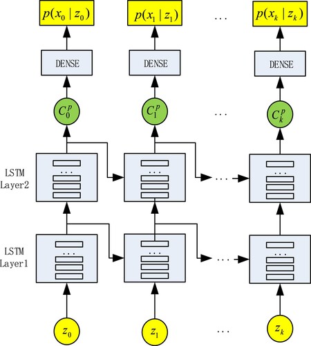
As shown in Figure 1, the designed LSTM network adopts a two-layer stacked LSTM network structure. The number of hidden states of each layer is consistent, which is represented by memory unit $C_k^P$. To avoid overfitting, each LSTM layer is followed by a Dropout layer. This is followed by the Dense layer which selects the Sigmoid activation function. The whole network structure is in the form of 1-to-1, which is to complete the posterior probability density estimation from the input target observation data $z_k$ to the target motion state $x_k$. See the simulation analysis section below for the specific settings of the network structure. The loss function of the network parameter optimization step is defined as follows: (20) $L(x,\hat{x},{\theta }_p)=\sum _{i=1}^T(x_i-{\hat{x}}_i|y_{i-1})$(20) After obtaining the posterior probability prediction result of the estimated motion state of the target of the current frame, formulas (12) and (13) of the above recursive accumulation step can be adjusted as follows: (21) $\begin{array}{rl}{I}_k(x_k)& =\underset{x_{k-1}\in \varphi ({\hat{x}}_k)}{max}\{\hat{P}(x_k|z_k)+I_{k-1}(x_{k-1})\}\end{array}$(21) (22) $\begin{array}{rl}{S}_k(x_k)& =\underset{x_{k-1}\in \varphi ({\hat{x}}_k)}{\arg max}\{\hat{P}(x_k|z_k)+I_{k-1}(x_{k-1})\}\end{array}$(22) Where, $\hat{P}(x_k|z_k)$ is the posterior probability density estimated by the LSTM network from each possible state transition point in the current k-th frame of the state transition set.

The main steps of the improved DP-TBD algorithm are as follows.

1. Initialization. When k = 1, (23) $\begin{array}{rl}{I}_1(x_1)& =\log p(z_1|x_1),\end{array}$(23) (24) $\begin{array}{rl}{S}_1(x_1)& =0,\end{array}$(24) (25) $\begin{array}{rl}{x}_1& =(p{x}_1,v{x}_1,a{x}_1,p{y}_1,v{y}_1,a{y}_1),\end{array}$(25)

2. Recursive accumulation. When $2\le k\le K$, for the state,

   1. Gets the set of state transitions $\phi ({\hat{x}}_k)$ for all possible positions from frame k-1 to frame k.

   2. All possible points in the state transition set are estimated with their corresponding posterior probability probability density through the above LSTM network.

   3. Find the maximum posterior probability value, and substitute it into formula (21) (22) as a function of the posterior probability value of the current frame and record its state transition relationship.

3. Termination of judgment. (26) $\begin{array}{rl}& {\stackrel{⌢}{x}}_k=\arg \underset{x_k\in R}{max}{I}_k(x_k),\end{array}$(26) (27) $\begin{array}{rl}s.t.I_k({\hat{x}}_k)& \succ V_k\end{array}$(27)

4. Track retracing. Letting $k=K-1,\dots ,1$, we have (28) ${\stackrel{⌢}{X}}_k=S_{k+1}(k+1),$(28)

5. Experiments

In this section, to demonstrated the tracking performance of the designed LSTM-DP-TBD algorithm for nonlinear small and weak targets, we use CS model simulation data and compare the tracking performance of our algorithm with that of the traditional DP-TBD algorithm for nonlinear dim targets under a series of different SNR conditions.

The current statistical model (CS) is a typical nonlinear motion model that can describe the motion state of a maneuvering target. It is able to effectively simulate the state change exhibited by the target when a maneuvering mutation occurs. The radar sampling period is set as T, and the state equation of the CS model is (29) $x_k=F(x_{k+1})+\overline{a}H+u_k,$(29) where F is the state transition matrix of the target, which is expressed as (30) $F_k=\left[\begin{array}{l}\phi \cdot 0_{3\times 3}\\ 0_{3\times 3}\cdot \phi \end{array}\right]$(30) where $0_{3\times 3}$ is a zero matrix with three rows and three columns, and the expression of $\mathrm{\Psi }$ is as follows: (31) $\mathrm{\Psi }=\left[\begin{array}{ccc}1& T& (e^{-\alpha T}+\alpha T-1)/{\alpha }^2\\ 0& 1& (-e^{-\alpha T}+1)/\alpha \\ 0& 0& e^{-\alpha T}\end{array}\right],$(31) where $\alpha$ is the maneuvering frequency, and the maneuverability reflected by the CS model varies with its value.

In Equation (31), $\overline{a}$ is the mean acceleration value. $u_k$ represents state noise that follows a normal distribution $u_k\sim N(0,{\sigma }_u^2)$. $H=[H_1{H}_2{]}^T$; $H_1$ and $H_2$ are expressed as: (32) $H_1=H_2=\left[\begin{array}{c}(1-\alpha T+{\alpha }^2{T}^2/2-e^{-\alpha T})/{\alpha }^2\\ (-1+\alpha T+e^{-\alpha T})/\alpha \\ 1-e^{-\alpha T}\end{array}\right],$(32) The target observation equation is (33) $z_k=\{\begin{array}{ll}{A}_k+v_k,& Y\\ v_k,& N\end{array},$(33) where the Y branch represents the case with the target at frame k, and the N branch represents the case without the target at frame k. $A_k$ is the target amplitude; $v_k$ represents observation noise and follows a normal distribution $v_k\sim N(0,{\sigma }_v^2)$.

The size of the radar observation area is set as $N_x\times N_y=100\times 100$, the resolution unit is $\mathrm{△}x=\mathrm{△}y=2$, the total frame length is $K=10$, and the radar scanning time interval is $T=1.2s$.

By using this model for simulation, a training dataset can be generated for training and testing the aforementioned LSTM network. Within a certain observation area, the initial state of the moving target is randomly set within a certain range. According to the state equation of the CS model mentioned above, 100 random target motion paths within a certain observation time are generated. And the corresponding observation sequences according to the observation equation of the CS model are also generated. The dimensions of the target state are the six dimensions mentioned above.

In the implementation of the LSTM network, a two-layer stacked LSTM network is adopted, and the number of hidden states in each layer is set to 256. To prevent overfitting, each LSTM layer is followed by a dropout layer with a ratio of 0.3. A 1-to-1 network structure is chosen. After this, 794,881 network parameters are set, and the best values of these parameters need to be found through training. The training loss function is the aforementioned loss function, and the adaptive moment estimation (Adam) optimization algorithm is adopted. The training dataset generated above is used to train and test the LSTM network.

In order to verify the detection and tracking performance of the architecture, the target observation data and corresponding truth stae values are randomly generated for verification under the CS model. The initial state of the target is set to $x_1=(8,4,0,6,3,0{)}^T$. The target is set to execute a strong steering maneuver in the observation area.

In this paper, the designed VL-DP-TBD algorithm is compared with the traditional DP-TBD algorithm in terms of the following aspects. (1) The amplitude distributions of the value function after K accumulation frames are compared to show the difference between the value function aggregation effects of the two algorithms. (2) The target detection probability Pd and tracking probability Pt are compared. Pd is defined as the probability of detecting the target after K accumulation frames, allowing for an error of one resolution unit. After detecting the target, Pt is defined as the probability that the estimated state obtained after track recovery is within one resolution unit of the real state in each frame. These probabilities are used to evaluate the detection and tracking performance of the two algorithms.

To this end, simulation experiment 1 is first carried out: when SNR = 10 dB is given, the value function distributions of the two DP-TBD algorithms are compared.

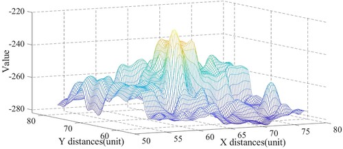
The value function distribution based on the traditional posterior probability value function of the DP-TBD algorithm is shown in Figure 2, the preset speed range is 3-0 times, and K frames are accumulated. As can be seen from the figure, the traditional DP-TBD algorithm produces an obvious agglomeration effect, which brings difficulties to the subsequent termination decision steps.

Figure 2. Amplitude distribution diagram of the traditional DP-TBD algorithm value function when the SNR is 10 dB.

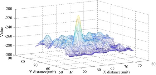
The value function distribution produced by the proposed VL-DP-TBD algorithm after K accumulation frames is shown in Figure 3. It can be seen from the figure that the new VL-DP-TBD algorithm is able to effectively suppress the agglomeration effect, and the value function obtained after K accumulation frames is highlighted.

Figure 3. Amplitude distribution diagram of the VL-DP-TBD algorithm value function when the SNR is 10 dB.

Second, simulation experiment 2 is carried out to compare the target detection probabilities Pd and tracking probabilities Pt of the two algorithms under a varying SNR. The results are obtained by conducting 2,000 Monte Carlo runs during the experiment.

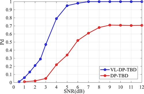
As shown in Figure 4, the detection probability Pd curves produced by the traditional DP-TBD algorithm and VL-DP-TBD algorithm as the SNR changes are compared. As can be seen from the figure, when the SNR is 2 dB, the Pd values of DP-TBD approache is close to 0, while that of VL-DP-TBD is close to 0.2. When the SNR is 1 dB, the Pd values of DP-TBD is close to 0, while that of VL-DP-TBD is close to 0.1. This proves that the VL-DP-TBD algorithm performs better in low SNR scenarios. When the SNR is greater than 2 dB, the Pd values of both methods begin to rise. When the SNR is higher than 5.2 dB, the Pd of the VL-DP-TBD algorithm rises to 1, while the Pd of the traditional DP-TBD algorithm tends to rise to 0.7 when the SNR is higher than 9 dB. Therefore, the detection performance of the VL-DP-TBD algorithm is obviously better than that of the traditional algorithm.

Figure 4. The detection probability curves produced by the two DP-TBD algorithms as the SNR changes.

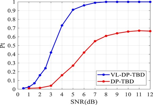
As shown in Figure 5, the tracking probability Pt curves produced by the traditional DP-TBD algorithm and the VL-DP-TBD algorithm as the SNR changes are compared. As can be seen from the figure, when the SNR is higher than 5.5 dB, the Pt of the VL-DP-TBD algorithm rises to 1, while the Pt of the traditional DP-TBD algorithm tends to rise to 0.65 when the SNR is higher than 9 dB. Therefore, the tracking performance of the VL-DP-TBD algorithm is better than that of the traditional algorithm.

Figure 5. The track probability curves produced by the two DP-TBD algorithms as the SNR changes.

6. Conclusion

In this paper, aiming at the problem that the traditional method is difficult to calculate in the generation of the posterior value function in the traditional DP-TBD algorithm, a designed LSTM network is used to directly obtain the estimated posterior probability function, and applied to the DP-TBD algorithm. A new VL-DP-TBD architecture is proposed. The improved architecture, whose value function calculation is no longer confined to the hypothetical probability distribution model, enhances its detection and tracking ability for non-cooperative nonlinear maneuvering dim small targets. The simulation results show that the proposed algorithm is superior in terms of suppressing the agglomeration effect and detection and tracking. However, VL-DP-TBD is only a preliminary algorithm, which can be further studied in terms of algorithm performance improvement and lightweight implementation in the future. With the promotion and application of intelligent chips for deep learning, it will be able to significantly improve the detection and tracking of non-cooperative weak and small slow targets in radar systems.

Author contributions

YL, WC, LD and FS conceived and designed the experiments; FS performed the experiments; FS, WC and LD analyzed the data; FS wrote the paper; YL administrated the project. All authors read and approved the final manuscript.

Availability of data and materials

Unfortunately, the data are not available online. Kindly, for data requests, please contact the corresponding author.

Declarations

Ethics approval and consent to participate

Not applicable.

Consent for publication

Approved.

Acknowledgments

The authors would like to express their sincere thanks to the editors and anonymous reviewers.

Disclosure statement

No potential conflict of interest was reported by the author(s).

Additional information

Funding

This work was funded by the Fundamental Research Funds for the Central Universities under grant 3102019ZX015 and in part by the Fundamental Research Funds for the Central Universities under grant D5000220131.

References

- Arlson, B. D., Evans, E. D., & Wilson, S. J. (1994). Search radar detection and track with the hough transform. I. System concept. IEEE Transactions on Aerospace and Electronic Systems, 30(1), 102–108. https://doi.org/10.1109/7.250410
- Arnold, J., Shaw, S. W., & Pasternack, H. (1993). Efficient target tracking using dynamic programming. IEEE Transactions on Aerospace and Electronic Systems, 29(1), 44–56. https://doi.org/10.1109/7.249112
- Barniv, Y., & Kella, O. (1985). Dynamic programming solution for detecting Dim moving targets. IEEE Transactions on Aerospace and Electronic Systems, AES-21(1), 144–156. https://doi.org/10.1109/TAES.1985.310548
- Barniv, Y., & Kella, O. (1987). Dynamic programming solution for detecting Dim moving targets part II: Analysis. IEEE Transactions on Aerospace and Electronic Systems, AES-23(6), 776–788. https://doi.org/10.1109/TAES.1987.310914
- Berclaz, J., Fleuret, F., Turetken, E., et al. (2011). Multiple object tracking using k-shortest paths optimization. IEEE Transactions on Pattern Analysis and Machine Intelligence, 33(9), 1806–1819. https://doi.org/10.1109/TPAMI.2011.21
- Boers, Y., & Driessen, H. (2003). A particle-filter-based detection scheme. Signal processing letters. IEEE, 10(10), 300–302.
- Buzzi, S., Lops, M., & Venturino, L. (2005). Track-before-detect procedures for early detection of moving target from airborne radars. IEEE Transactions on Aerospace and Electronic Systems, 41(3), 937–954. https://doi.org/10.1109/TAES.2005.1541440
- Chenouard, N., Bloch, I., & Olivo-Marin, J. C. (2013). Multiple hypothesis tracking for cluttered biological image sequences. IEEE Transactions on Software Engineering, 35(11), 2736–2750.
- Davey, S. J. (2012). Comments on “joint detection and estimation of multiple objects from image observations”. IEEE Transactions on Signal Processing, 60(3), 1539–1540. https://doi.org/10.1109/TSP.2011.2173679
- Fu, J., Zhang, H., Luo, W., Gao, X. (2022). Dynamic programming ring for point target detection. Applied Sciences, 12(3), 1151. https://doi.org/10.3390/app12031151
- Gers, F. A., Schmidhuber, J., & Cummins, F. (2000). Learning to forget: Continual prediction with LSTM. Neural Computation, 12(10), 2451–2471. https://doi.org/10.1162/089976600300015015
- Greff, K., Srivastava, R. K., Koutník, J., Steunebrink, B. R., Schmidhuber, J. (2017). LSTM: A search space odyssey. IEEE Transactions on Neural Networks and Learning Systems, 28(10), 2222–2232. https://doi.org/10.1109/TNNLS.2016.2582924
- Hochreiter, S., & Schmidhuber, J. (1997). Long short-term memory. Neural Computation, 9(8), 1735–1780. https://doi.org/10.1162/neco.1997.9.8.1735
- Johnston, L. A., & Krishnamurthy, V. (2002). Performance analysis of a dynamic programming track before detect algorithm. IEEE Transactions on Aerospace and Electronic Systems, 38(1), 228–242. https://doi.org/10.1109/7.993242
- Li, C., Bai, X., Zhao, J., Shan, T. (2022). An effective method for weak multi-target detection and tracking in clutter environment, in Proceedings of the 6th International Conference on Digital Signal Processing (ICDSP ‘22). Association for Computing Machinery, 134–139. https://doi.org/10.1145/3529570.3529593
- Lu, X., Cheng, T., Deng, M., Wang, Z., He, Z., Li, H. (2022). A novel track -before-detect algorithm for airborne target with over-the-horizon radar. in 2022 IEEE Radar Conference (RadarConf22), 01–06. https://doi.org/10.1109/RadarConf2248738.2022.9764334
- Perello-March, J. R., Burns, C. G., Woodman, R., Elliott, M. T., Birrell, S. A. (2021). Driver state monitoring: Manipulating reliability expectations in simulated automated driving scenarios. IEEE Transactions on Intelligent Transportation Systems, 99, 1–11.
- Rutten, M. G., Gordon, N. J., & Maskell, S. (2005). Recursive track-before-detect with target amplitude fluctuations. Radar, sonar and navigation. IEE Proceedings, 152(5), 345–352. http:///10.1049/ip-rsn_20045041.
- Tonissen, S. M., & Evans, R. J. (1996). Peformance of dynamic programming techniques for track-before-detect. IEEE Transactions on Aerospace and Electronic Systems, 32(4), 1440–1451. https://doi.org/10.1109/7.543865
- Wang, S., & Zhang, Y. (2016). Improved dynamic programming algorithm for low SNR moving target detection. Syst. Eng. Electron, 38(1), 2244–2251. http://10.3969/j.issn.1001-506X.2016.10.04.
- Wen, L. W., Ding, J. S., Cheng, Y., & Xu, Z. (2022). Dually supervised track-before-detect processing of multichannel video SAR data. IEEE Transactions on Geoscience and Remote Sensing, 60(1), 238–252. http://10.1109/TGRS.2022.3178636
- Williams, R. J., & Peng, J. (1990). An efficient gradient-based algorithm for On-line training of recurrent network trajectories. Neural Computation, 10(4), 490–501. http://10.1162/neco.1990.2.4.490
- Xing, H., Suo, J., & Liu, X. (2020). A dynamic programming track-before-detect algorithm with adaptive state transition set. In International Conference in Communications, Signal Processing, and Systems; Springer: Singapore. 638–646.
- Yi, W. (2012). Research on track-before-detect algorithms for multiple-target detection and tracking. Dissertation, Chengdu: University of Electronic Science and Technology of China, 44–46.
- Yi, W., Morelande, M. R., Kong, L.-J., Yang, J. -Y., Deng, X. -B., (2012). Multi-target tracking via dynamic-programming based track-before-detect, in proceedings of the radar conference (RADAR). IEEE, 487–492. http://10.1109/RADAR.2012.6212190
- Zheng, D., Wang, S., & Liu, C. (2014). An improved dynamic programming track-before-detect algorithm for radar target detection. In 2014 12th International Conference on Signal Processing (ICSP), 2120–2124. https://doi.org/10.1109/ICOSP.2014.7015369
- Zhu, Y. R., Li, Y., Zhang, N., Zhang, Q. M., (2022). Candidate-plots-based dynamic programming algorithm for track-before-detect. Digital Signal Processing, 123, 1051–2004. https://doi.org/10.1016/j.dsp.2022.103458