Camera calibration method based on circular array calibration board

Abstract

Camera calibration will directly affect the accuracy and stability of the whole measurement system. According to the characteristics of circular array calibration plate, a camera calibration method based on circular array calibration plate is proposed in this paper. Firstly, subpixel edge detection algorithm is used for image preprocessing. Then, according to cross ratio invariance and geometric constraints, the projection point position of the center point is obtained. Finally, the calibration experiment was carried out. Experimental results show that under any illumination conditions, the average reprojection error of the center coordinates obtained by the improved calibration algorithm is less than 0.12 pixels, which is better than the traditional camera calibration algorithm.

KEYWORDS:

• Systems identification and signal processing
• Image processing and vision
• Theory-framework
• Least squares methods
• Theory-framework
• Optimal estimation

1. Introduction

With the continuous expansion of computer vision application fields, the application scenarios of 3D vision measurement are also expanding. Cameras are the most important sensors in machine vision, which has a wide range of applications in artificial intelligence (Graves et al., 2009), vision measurement (Huang et al., 2017; Kanakam, 2017; Liu et al., 2017), and robotics technology (Kahn et al., 1990; Yang et al., 2007). As a key technology of visual measurement, camera calibration plays a key role in the fields of machine vision ranging, pose estimation, and three-dimension (3D) reconstruction (Liu, 2001). The calibration process establishes the transformation relationship from the 3D image coordinate system to the 3D world coordinate system (Sang, 2021). The accuracy of calibration parameters directly affects the accuracy of vision applications (Chen, 2020; Huang et al., 2020; Li et al., 2020). Presently, domestic and foreign scholars have carried out extant research on camera calibration technology and have proposed many camera calibration algorithms (Qiu et al., 2000; Zhang et al., 2019).

On the basis of the different number of vision sensors, existing camera calibration methods can be divided into monocular vision camera calibration, binocular vision camera calibration, and multi-vision camera calibration. On the basis of the different calibration methods, the camera calibration methods can usually be divided into three types namely, calibration method based on calibration template (Tsai, 1986), calibration method based on active vision (Maybank & Faugeras, 1992), and camera self-calibration method (Zhang & Tang, 2016). The so-called calibration method based on calibration template uses a calibration object with a known structure and high-precision as a spatial reference, establishes the constraint relationship between camera model parameters through the correspondence between spatial points, and solves these parameters on the basis of the optimal algorithm. parameter. Typical representative methods include direct linear transformation (DLT) (Abdel-Aziz, 2015) and Tsai two-step method (Tsai, 1986). The calibration method based on the calibration template can obtain calibration with relatively high accuracy, but the processing and maintenance of the calibration object is complicated, and setting the calibration object in the harsh and dangerous actual operating environment is difficult. The camera calibration method based on active vision refers to obtaining multiple images by actively controlling the camera to perform some special motions on a platform that can be precisely controlled and using the images collected by the camera and the motion parameters of the controllable camera to determine the camera parameters. The representative method of this class is the linear method based on two sets of three orthogonal motions proposed by Massonde (Sang, 1996). Subsequently, Yang et al. proposed an improved scheme, that is, based on four groups of plane orthogonal motion and give groups of plane orthogonal motion, the camera is linearly calibrated by using the pole information in the image (Li et al., 2000; Yang et al., 1998). This calibration method is simple to calculate and can generally be solved linearly and has good robustness, but the system cost is high, and it is not applicable when the camera motion parameters are unknown or the camera motion cannot be precisely controlled. In recent years, the camera self-calibration method proposed by many scholars can independently calibrate the reference object by only using the correspondence between multiple viewpoints and the surrounding environment during the natural movement of the camera. This method has strong flexibility and high applicability, and it is usually used for camera parameter fitting based on absolute quadric or its dual absolute quadric (Wu & Hu, 2001). However, this method belongs to nonlinear calibration, and the accuracy and robustness of the calibration results are not high.

The camera calibration method of Zhang (Zhang, 1999) requires shooting checkerboard calibration board images from several angles. Because this method is simple and effective which is often used in camera calibration processes. However, in calibrating with checkerboard, the accuracy of corner extraction is greatly affected by noise and image quality (Wu et al., 2013), whereas circular features are not sensitive to segmentation thresholds, the recognition rate is relatively high, and the projection of circles image noise has a strong known effect (Crombrugge et al., 2021), so circular features have good application prospects in vision systems (Rudakova & Monasse, 2014). In the perspective projection transformation, when the circular feature calibration plate is used for calibration, the collected circle will be transformed into an ellipse (referred to as a projection ellipse). Presently, the positioning of projected ellipse has become a research hotspot in machine vision (Zhang et al., 2017), and its positioning accuracy will directly affect the camera calibration accuracy and object measurement accuracy. The commonly used algorithms for ellipse extraction at this stage are Canny detection least squares ellipse fitting method (Wang et al., 2016), Hough transform method (Bozomitu et al., 2016; Ito et al., 2011), gray centre of gravity (Frosio & Borghese, 2008), Hu invariant moment (Hu, 1962), and other methods. The Hough transform method has good anti-noise and strong robustness, but has a large amount of storage, high computational complexity, and poor pertinence; the gray-scale centroid method requires uniform gray levels, otherwise the error will be large (Zhang et al., 2017); Canny detection is the smallest. The quadratic ellipse fitting method is fast and accurate (Wang et al., 2016). Zhu et al. (Zhu et al., 2014) used the asymmetric projection of the circle’s centre to calculate the centre coordinates of the ellipse after projection. The theoretical value and the actual value in the image are matched by least squares, but the internal parameters of the camera cannot be assumed in practical applications, and the scope of application is small. Wu et al. (Wu et al., 2018) proposed a circular mark projection eccentricity compensation algorithm based on three concentric circles, which is calculated according to the eccentricity model of three groups of ellipse fitting centre coordinates and the amount of calculation is large; Lu et al. (Lu et al., 2020) proposed a high-precision camera calibration method based on the calculation of the real image coordinates of the centre of the circle, which obtains the true centre of the circle through multiple iterative calculations. However, the projection process is relatively complex and requires a large amount of computation; Xie et al. (Xie & Wang, 2019) proposed a circle centre extraction algorithm based on geometric features of dual quadratic curves, but the computational complexity is large; Peng et al. (Peng et al., 2022) proposed a method of plane transformation, which uses front and back perspective projection to obtain the coordinates of the landmark points, but it requires more manual work when selecting corner points and adjusting parameters. Aiming at the characteristics of the circular calibration plate, this paper proposes a camera calibration method on the basis of the circular array calibration plate. First, the sub-pixel edge detection algorithm is used to detect the edge of the preprocessed image, then, according to the principle of finding the centre of the ellipse according to the geometric constraints of the plane, the equation system is established to solve the position of the projection point of the circle’s centre, and finally, Zhang’s plane-based camera is used according to the coordinates of the circle’s centre. Calibration method for camera calibration. The experimental results show that the combination of the ellipse contour extraction algorithm and Zhang’s camera calibration method can obtain higher camera calibration accuracy.

2. Image acquisition and preprocessing

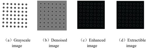
This article uses the thousand-eyed wolf 30 W pixel camera of Fuhuang Junda Hi-Tech to take pictures and collect images. First, the camera is fixed on the stand and stand still, then, the calibration plate is moved and rotated with a 7 × 7 dot array, and 14 pictures of the calibration plate are taken with different poses and directions, 12 of which are shown in Figure 1. First, the collected image is converted into a grayscale image, then, the grayscale image is edge preserved and denoized through guided filtering, next, the image sharpening algorithm is used to highlight the circular markers in the image, and then the Canny operator is used to detect the image edge. Finally, the sub-pixel edge detection algorithm is used for edge detection, and the results are shown in Figure 2, which are (a) grayscale image, (b) denoised image, (c) enhanced image, and (d) extractible image.

Figure 1. 12 Calibration board images with different pose and direction.

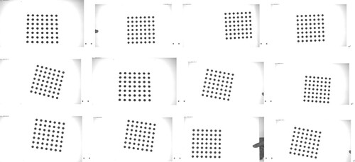
Figure 2. Pretreatment images.

In the perspective projection transformation, when the circular feature calibration plate is used for calibration, the collected circle will be transformed into an ellipse because it is in a non-parallel state with the camera. In this paper, the sub-pixel edge detection algorithm is used to detect the edge of the collected image. Then, the circularity, eccentricity, and convexity conditions are restricted according to the characteristics of the obtained closed edge to extract the ellipse contour that meets the requirements.

1. Roundness

The roundness feature reflects the degree to which the figure is close to a perfect circle, and its range is $\left(0,1\right)$. The circularity $C$ can be expressed as. (1) $C=4\pi \left(S/P^2\right)$(1) Among them, $S$ and $P$ represent the area and perimeter of the graphic shape, respectively. When the circularity $C$ is 1, it means that the graphic shape is a perfect circle, and when the circularity $C$ is 0, it means that the shape is a gradually elongated polygon. Therefore, the closer the feature points to be extracted in this paper are to a circle, the closer the value of circularity $C$ is to 1.

1. Eccentricity

Eccentricity is the degree to which a conic deviate from an ideal circle. The eccentricity of an ideal circle is 0, so the eccentricity represents how different the curve is from the circle. The greater the eccentricity, the less camber of the curve. Among them, an ellipse with an eccentricity between 0 and 1 is an ellipse, and an eccentricity equal to 1 is a parabola. Given that directly calculating the eccentricity of a graphic is complicated, the concept of image moment can be used to calculate the inertial rate of the graphic, and then the eccentricity can be calculated from the inertial rate. The relationship between the eccentricity $E$ and the inertia rate $I$ is: (2) $E^2+I^2=1$(2) In the formula, the eccentricity of the circle is equal to 0, and the inertia rate is equal to 1. The closer the inertia rate is to 1, the higher the degree of the circle.

1. Convexity

For a figure and any two points A and B located in the figure F, if all the points on the line segment AB are always located in the figure, the figure is called a convex figure, otherwise, the figure is called a concave figure. Convexity is the degree to which a polygon is close to a convex figure, and the convexity $V$ is defined as: (3) $V=S/H$(3) In the formula, $H$ represents the convex hull area corresponding to the figure. The closer the convexity is to 1, the closer the figure is to a circle.

3. Precise positioning algorithm of the projection point of the circle’s centre

3.1. Projection model of the space circle on camera imaging plane

Let the position of the circle’s centre be the origin of the world coordinate system, the $Z$ axis of the world coordinate system is perpendicular to the plane where the circular pattern is located, and the plane where the graphic pattern is located is the plane of the world coordinate system. Suppose the radius of the circle is r, so the equation of the circle in the plane of the world coordinate system is, then the matrix $C$ is expressed as. (4) $\left[\begin{array}{ccc}x& y& 1\end{array}\right]\left[\begin{array}{ccc}1& 0& 0\\ 0& 1& 0\\ 0& 0& -r^2\end{array}\right]\left[\begin{array}{c}x\\ y\\ 1\end{array}\right]=\left[\begin{array}{ccc}x& y& 1\end{array}\right]C\left[\begin{array}{c}x\\ y\\ 1\end{array}\right]$(4) The general formal equation of an ellipse can be expressed as, which is organized into a matrix form and represented by a matrix $E$. (5) $E=\left[\begin{array}{ccc}a& c/2& d/2\\ c/2& b& e/2\\ d/2& e/2& f\end{array}\right]$(5)

3.2. Projective geometry theory

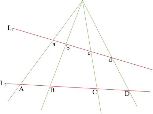
If the camera distortion is ignored, the camera imaging is the projective transformation of the calibration plate plane, and the properties of the projective transformation can be used to calculate the transformation relationship between the imaging plane and the calibration plate plane. Among them, the intersection ratio is a basic invariant in projective geometry. If four collinear points, $A$, $B$, $C$, and $D$ exist, in the plane, their intersection ratio can be written as: (6) $\left(A,B;C,D\right)=\frac{\left(A,B,C\right)}{\left(A,B,D\right)}=\frac{||AC||/||BC||}{||AD||/||BD||}$(6) On the basis of the projective transformation diagram, the four collinear points $\text{a}$, $\text{b}$, $\text{c}$, and d on the straight line ${\text{L}}_{\text{1}}$ are mapped to the four collinear point, $A$, $B$, $C$, and $D$ on the straight line ${\text{L}}_{\text{2}}$, then: (7) $\left(A,B;C,D\right)=\left(a,b;c,d\right)={\lambda }_1/{\lambda }_2$(7) A schematic of the transformation is shown in Figure 3.

Figure 3. Schematic diagram of projective transformation.

Particularly, when $\left(A,B,C,D\right)=-1$, the cross ratio is called the harmonic ratio, and the four collinear points, $A$, $B$, $C$, and $D$, are called harmonic conjugates. If point $C$ is the midpoint of $AB$ and point $D$ among the four collinear points satisfying the harmonic ratio is an infinite point in the direction of the straight line where points $A$ and $B$ are located, then the four collinear points, $A$, $B$, $C$, and $D$, are harmonically conjugated. Thus, $C$, and $D$ can be expressed as. (8) $\{\begin{array}{l}C=A+{\lambda }_{1}B\\ D=A+{\lambda }_{2}B\end{array}$(8) If the four collinear points, $A$, $B$, $C$, and $D$, are harmonically conjugated, then there is ${\lambda }_1/{\lambda }_2=-1$. When the four collinear points $A$, $B$, $C$, and $D$ are harmonically conjugated, there is ${\lambda }_1=-{\lambda }_2$.

The equation of the infinite line in the plane where the inner circle of the world coordinate system is located is $l_{\mathrm{\infty }}=[0,0,1{]}^T$, and the equation of the projected line on the imaging plane is $l{}_{\mathrm{\infty }}^{\mathrm{\prime }}=H^{-T}{l}_{\mathrm{\infty }}=H^{-T}\left[\begin{array}{c}0\\ 0\\ 1\end{array}\right]$. The projection point of the centre O on the imaging plane is $O^{\mathrm{\prime }}=HO$. According to Formula (2), the product of the projected ellipse equation E and the projected point O’ at the circle’s centre is. (9) $E{O}^{\mathrm{\prime }}=H^{-T}C{H}^{-1}HO=H^{-1}CO=H^{-1}\left[\begin{array}{ccc}1& 0& 0\\ 0& 1& 0\\ 0& 0& r^2\end{array}\right]\left[\begin{array}{c}0\\ 0\\ 1\end{array}\right]$(9)

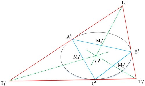
3.3. Geometric constraints

An inscribed triangle of the circle is drawn on the perfect circle image of the calibration plate. The intersection points with the circle are points $A$, $B$ and $C$. The tangent of the circle is drawn at three points $A$, $B$ and $C$, and their intersection points are $T_1$, $T_2$, and $T_3$, respectively, assuming that $M_1$, $M_2$, and $M_3$ are the midpoints of the chords $AC$, $BC$, and $AB$. According to geometric knowledge, the intersection of the tangent to the circle and the midpoint of the corresponding chord passes through the circle’s centre. During projective transformation, this property does not change. In addition, the projection of a straight line remains a straight line, and the tangent of a circle remains tangent to the projected ellipse in the imaging plane (Wu & Hu, 2001). Therefore, in the projection ellipse, the line connecting the tangent intersection points ${T_1}^{\mathrm{\prime }}$, ${T_2}^{\mathrm{\prime }}$, ${T_3}^{\mathrm{\prime }}$ and the corresponding projection points ${M_1}^{\mathrm{\prime }}$, ${M_2}^{\mathrm{\prime }}$, ${M_3}^{\mathrm{\prime }}$ must intersect at a point O’, which is the projection point of the circle’s centre on the imaging plane. A schematic is shown in Figure 4.

Figure 4. Geometric constraint relationship.

3.4. Calculation of the projection point of the real centre of the circle

After the grayscale processing of the image captured by the camera, the Otsu method is used first to obtain the binary segmentation threshold, and the image is processed to be binarized. Given that the pattern on the calibration plate is usually a black circle on a white background, for convenience, the binary image is inverted, and the pixels belonging to the projected ellipse area are marked as 1. After the connected domain is extracted, the boundary tracking algorithm is executed to obtain the boundary point set of the projected ellipse in the image. On the basis of the extracted boundary point set, the ellipse equation is fitted by the method of ellipse direct least square fitting, and the general equation of ellipse $a{x}^2+b{y}^2+cxy+dx+ey+f=0$ is obtained.

The knowledge of plane geometry demonstrates that the general equation of ellipse $E$ is $a{x}^2+b{y}^2+cxy+dx+ey+f=0$ (a, b, c, d, e, f are known quantities), any point P on ellipse $E$ is taken, and the tangent of ellipse $E$ is drawn through this point, when this tangent slope exists, the slope is $k_i=-\frac{2a{x}_i+b{y}_i+d}{b{x}_i+2c{y}_i+e}\left(i=1,2,3\dots \right)$.

The coordinates of the feature points, $A^{\mathrm{\prime }}$, $B^{\mathrm{\prime }}$ and $C^{\mathrm{\prime }}$, can be extracted from the collected images, and their homogeneous coordinates may be set as $\left(x_1,y_1,z_1\right)$, $\left(x_2,y_2,z_2\right)$ and $\left(x_3,y_3,z_3\right)$, respectively. According to the mathematical knowledge of plane geometry, the equation of the tangent line passing through points $A^{\mathrm{\prime }}$, $B^{\mathrm{\prime }}$ and $C^{\mathrm{\prime }}$ can be expressed as a point-slope equation as. (10) $\{\begin{array}{l}{l}_1:y-y_1=k_1\left(x-x_1\right)\\ l_2:y-y_2=k_2\left(x-x_2\right)\\ l_3:y-y_3=k_3\left(x-x_3\right)\end{array}$(10) From this, the coordinates of the intersection points, ${T_1}^{\mathrm{\prime }}$, ${T_2}^{\mathrm{\prime }}$, and ${T_3}^{\mathrm{\prime }}$, of the tangent lines can be obtained.

Let the homogeneous coordinates of ${M_1}^{\mathrm{\prime }}$, ${M_2}^{\mathrm{\prime }}$, ${M_3}^{\mathrm{\prime }}$ be. (11) $\{\begin{array}{l}{M_1}^{\mathrm{\prime }}:A^{\mathrm{\prime }}+\alpha C^{\mathrm{\prime }}=\left(x_1+\alpha x_3,y_1+\alpha y_3,1+\alpha \right)\\ {M_2}^{\mathrm{\prime }}:C^{\mathrm{\prime }}+\text{β}{B}^{\mathrm{\prime }}=\left(x_3+\text{β}{x}_2,y_3+\text{β}{y}_2,1+\text{β}\right)\\ {M_3}^{\mathrm{\prime }}:B^{\mathrm{\prime }}+\gamma A^{\mathrm{\prime }}=\left(x_2+\gamma x_1,y_2+\gamma y_1,1+\gamma \right)\end{array}$(11) where $\alpha$, $\text{β}$ and $\gamma$ are unknown quantities.

Let the infinity points of the straight lines be $A^{\mathrm{\prime }}{C}^{\mathrm{\prime }}$, $A^{\mathrm{\prime }}{B}^{\mathrm{\prime }}$ and $B^{\mathrm{\prime }}{C}^{\mathrm{\prime }}$ be ${V_1}^{\mathrm{\prime }}$, ${V_2}^{\mathrm{\prime }}$ and ${V_3}^{\mathrm{\prime }}$ respectively. According to Formula (8), we have. (12) $\{\begin{array}{l}{V_1}^{\mathrm{\prime }}-A^{\mathrm{\prime }}-\alpha C^{\mathrm{\prime }}=\left(x_1-\alpha x_3,y_1-\alpha y_3,1-\alpha \right)\\ {V_2}^{\mathrm{\prime }}:C^{\mathrm{\prime }}-\text{β}{B}^{\mathrm{\prime }}=\left(x_3-\text{β}{x}_2,y_3-\text{β}{y}_2,1-\text{β}\right)\\ {V_3}^{\mathrm{\prime }}:B^{\mathrm{\prime }}-\gamma A^{\mathrm{\prime }}=\left(x_2-\gamma x_1,y_2-\gamma y_1,1-\gamma \right)\end{array}$(12) In the projective transformation, the projection points of the infinity points in the direction of the straight line where the three chords are located are collinear, then there are: (13) ${V_2}^{\mathrm{\prime }}\bullet \left[{V_1}^{\mathrm{\prime }}\times {V_3}^{\mathrm{\prime }}\right]=0$(13) Let the straight lines, ${T_1}^{\mathrm{\prime }}{M_1}^{\mathrm{\prime }}$, ${T_2}^{\mathrm{\prime }}{M_2}^{\mathrm{\prime }}$, ${T_3}^{\mathrm{\prime }}{M_3}^{\mathrm{\prime }}$, be the straight lines, $L_1$, $L_2$, and $L_3$, respectively, because the coefficient vector of the equation connecting the two points in the projective plane is the cross product of the homogeneous coordinate vectors of the two points, the homogeneous coordinates of the intersection of the two straight lines are the cross product of the coefficient vectors of the straight line equations, so the coefficient vectors of the straight lines, $L_1$, $L_2$, and $L_3$ are. (14) $\{\begin{array}{l}{L}_1={T_1}^{\mathrm{\prime }}\times {M_1}^{\mathrm{\prime }}\\ L_2={T_2}^{\mathrm{\prime }}\times {M_2}^{\mathrm{\prime }}\\ L_3={T_3}^{\mathrm{\prime }}\times {M_3}^{\mathrm{\prime }}\end{array}$(14) From the geometric relationship, the three lines, $L_1$, $L_2$, and $L_3$, have the same point, then there are: (15) $L_2\bullet \left[L_1\times L_3\right]=0$(15) The intersection of $L_2$ and $L_3$ is the centre projection point O’, $O^{\mathrm{\prime }}=L_2\times L_3$. The projection of the infinite straight line of the plane where the circle is located on the imaging plane is a finite straight line. Formula (5) demonstrates that the projection equation is: (16) ${l_{\mathrm{\infty }}}^{\mathrm{\prime }}=E{O}^{\mathrm{\prime }}=E\bullet \left[L_2\times L_3\right]$(16) Given that all infinity points are on this infinity straight line, the point V₃’ is on ${l_{\mathrm{\infty }}}^{\mathrm{\prime }}$, then we have: (17) ${l_{\mathrm{\infty }}}^{\mathrm{\prime }}\bullet {V_3}^{\mathrm{\prime }}=0$(17) Formulas (13), (15), and (17) are combined to obtain a nonlinear equation system containing three unknowns $\alpha$, $\text{β}$ and $\gamma$, and this nonlinear equation system is solved to obtain the values of $\alpha$, $\text{β}$ and $\gamma$, and $\alpha$, $\text{β}$ and $\gamma$ into the expressions of the straight lines $L_1$, $L_2$, and $L_3$ to obtain the coordinates of the projection point of the circle’s centre.

4. Camera calibration

Camera calibration is to determine the correspondence between a certain point in space and its position in a 2D image by calculating the camera’s internal parameters and external coordinate system position parameters. The calibration method used in this paper is Zhang’s plane calibration method. In the imaging geometry of the camera, the linear imaging model of the camera describes the imaging process based on four coordinate systems, which are the world coordinate system, the camera coordinate system, the image physical coordinate system, and the image pixel. Coordinate System. Let the homogeneous coordinate of the world coordinate system of a point P in space is ${\left[\begin{array}{cccc}{X}_w& Y_w& Z_w& 1\end{array}\right]}^T$, the coordinate of the rigid body transformed into the camera coordinate system is ${\left[\begin{array}{ccc}{X}_c& Y_c& Z_c\end{array}\right]}^T$, the coordinate of the perspective projection into the image imaging coordinate system is ${\left[\begin{array}{ccc}x& y& z\end{array}\right]}^T$, and the corresponding pixel coordinate of the final projection into the image is $\left[\begin{array}{cc}u& v\end{array}\right]$. The transformation relationship between the world coordinate system and the image coordinate system can be obtained through the transformation between these four coordinate systems. (18) $\begin{array}{rl}& \left[\begin{array}{c}u\\ v\\ 1\end{array}\right]=\left[\begin{array}{ccc}{k}_u& 0& u_0\\ 0& k_v& v_0\\ 0& 0& 0\end{array}\right]\left[\begin{array}{c}x\\ y\\ 1\end{array}\right]\end{array}$(18) (19) $\begin{array}{rl}& \left[\begin{array}{c}x\\ y\\ 1\end{array}\right]=\left[\begin{array}{ccc}{f}_x& 0& 0\\ 0& f_y& 0\\ 0& 0& 1\end{array}\right]\left[\begin{array}{c}{X}_c\\ Y_c\\ Z_c\end{array}\right]\end{array}$(19) In the formula, $H_1$ is the internal parameter matrix, ${\text{f}}_{\text{x}}$, ${\text{f}}_{\text{y}}$, ${\text{u}}_{\text{0}}$, ${\text{v}}_{\text{0}}$ are the parameters of the internal parameter matrix, and ${\text{k}}_{\text{u}}$ and ${\text{k}}_{\text{v}}$ are the scale factors on the X-axis and Y-axis, respectively.

In summary, the conversion relationship between the world coordinate system and the pixel coordinate system can be expressed as (20) $\begin{array}{rl}{Z}_c\left[\begin{array}{c}u\\ v\\ 1\end{array}\right]& =\left[\begin{array}{cccc}{f}_x& 0& u_0& 0\\ 0& f_y& v_0& 0\\ 0& 0& 1& 0\end{array}\right]\left[\begin{array}{cc}R& T\\ 0^T& 1\end{array}\right]\left[\begin{array}{c}{X}_w\\ Y_w\\ Z_w\\ 1\end{array}\right]\\ & =H_1{H}_2\left[\begin{array}{c}{X}_w\\ Y_w\\ Z_w\\ 1\end{array}\right]=H\left[\begin{array}{c}{X}_w\\ Y_w\\ Z_w\\ 1\end{array}\right]\end{array}$(20) In the formula: ${\text{Z}}_{\text{c}}$ is the Z-axis coordinate value in the camera coordinate system, and $R$ and $T$ represent the rigid body transformation. $H$ is a homography matrix, which contains the camera internal parameter matrix $H_1$ and the external parameter matrix $H_2$. The internal parameter matrix is only related to the camera’s own attributes and internal structure; the external parameter matrix is completely determined by the mapping relationship between the world coordinate system and the camera coordinate system.

Assuming that the ideal pixel coordinate is $\left(\begin{array}{cc}u& v\end{array}\right)$, because the camera is distorted during the shooting process, the real pixel coordinate is $\left(\begin{array}{cc}\stackrel{⌢}{u}& \stackrel{⌢}{v}\end{array}\right)$. Nonlinear distortion is mainly divided into radial distortion, tangential distortion, and centrifugal distortion, whereas Zhang’s plane calibration method only considers radial distortion. To improve the accuracy of camera calibration, this paper not only obtains the radial distortion coefficients k₁, k₂, and k₃ during calibration, but also obtains two tangential distortion coefficients p1 and p2. The nonlinear distortion model can be expressed as. (21) $\{\begin{array}{l}\stackrel{⌢}{x}=x+x\left[k_1\left(x^2+y^2\right)+k_2{\left(x^2+y^2\right)}^2+k_3{\left(x^2+y^2\right)}^4\right]\\ +\left[p_1\left(3x^2+y^2\right)+2p_{2}xy\right]\\ \stackrel{⌢}{y}=y+y\left[k_1\left(x^2+y^2\right)+k_2{\left(x^2+y^2\right)}^2+k_3{\left(x^2+y^2\right)}^4\right]\\ +\left[p_2\left(3x^2+y^2\right)+2p_{1}xy\right]\end{array}$(21) In the formula,$\left(\begin{array}{cc}x& y\end{array}\right)$ and $\left(\begin{array}{cc}\stackrel{⌢}{x}& \stackrel{⌢}{y}\end{array}\right)$ represent the coordinates of $\left(\begin{array}{cc}u& v\end{array}\right)$ and $\left(\begin{array}{cc}\stackrel{⌢}{u}& \stackrel{⌢}{v}\end{array}\right)$ in the image coordinate system, respectively. The radial distortion coefficients k₁, k₂, k₃ and the tangential distortion coefficients p1, p2 can be obtained by using the least square method.

5. Calibration results and analysis

The experimental operating platform used in this article is mainly Lenovo computer, which has a 64 bit Windows 10 system and an Intel (R) Core (TM) i7-10700 processor [email protected] GHz. The resolution of the camera used in the experiment is 1920 × 1080 pixels. The checkerboard calibration board is a 12 * 9 grid, with each grid size of 14 mm * 14 mm. The circular array calibration plate is a 7 * 7 dot with a diameter of 5.0 mm and a centre distance of 10.0 mm. First, 14 images collected by the camera are preprocessed, and VS2019 and OpenCV4.5 are used to read the processed images into the written C++ program. By extracting the centres of all circles in 14 images and comparing them with the 3D space of the centres on the calibration board, corresponding values and calibration results are obtained. Other experimental conditions remain unchanged. Under three lighting conditions, 14 chessboard calibration images are also collected for calibration. Therefore, the experimental results are as follows. The camera internal parameter matrices are:

1. Uneven illumination (Table 1 and Table 2): $\begin{array}{rl}{H}_{1\text{circular array}}& =[\begin{array}{cc}4896.563707& 0\\ 0& 4893.757057\\ 0& 0\end{array}\\ & \begin{array}{c}774.879906\\ 549.748346\\ 1\end{array}]\end{array}$ $\begin{array}{rl}{H}_{1\text{checkerboard}}& =[\begin{array}{cc}4871.170691& 0\\ 0& 4882.933311\\ 0& 0\end{array}\\ & \begin{array}{c}950.355523\\ 440.277167\\ 1\end{array}]\end{array}$

2. Strong illumination (Table 3 and Table 4): $\begin{array}{rl}{H}_{1\text{circular array}}& =[\begin{array}{cc}4996.563707& 0\\ 0& 4993.757057\\ 0& 0\end{array}\\ & \begin{array}{c}704.562029\\ 588.646041\\ 1\end{array}]\end{array}$ $\begin{array}{rl}{H}_{1\text{checkerboard}}& =[\begin{array}{cc}4995.705161& 0\\ 0& 4986.210450\\ 0& 0\end{array}\\ & \begin{array}{c}996.259745\\ 553.611204\\ 1\end{array}]\end{array}$

3. Weak illumination (Table 5 and Table 6): $\begin{array}{rl}{H}_{1\text{circular array}}& =[\begin{array}{cc}4999.048416& 0\\ 0& 4994.348380\\ 0& 0\end{array}\\ & \begin{array}{c}629.362277\\ 584.669272\\ 1\end{array}]\end{array}$ $\begin{array}{rl}{H}_{1\text{checkerboard}}& =[\begin{array}{cc}4995.705161& 0\\ 0& 4986.210450\\ 0& 0\end{array}\\ & \begin{array}{c}895.582206\\ 573.315153\\ 1\end{array}]\end{array}$

The difference between ${\text{f}}_{\text{x}}$ and ${\text{f}}_{\text{y}}$ is not significant, and the radial distortion coefficient and tangential distortion coefficient are not large. To test the accuracy and feasibility of the calibration results, this paper adopts re-projection error calculation. First, the high-precision pixel coordinates of the circle’s centre are obtained on the basis of the algorithm proposed in this paper, and then using the correspondence between the pixel coordinate system and the world coordinate system mentioned above, the coordinates are reprojected to obtain the corresponding reprojected pixel coordinate values. Among them, the circular coordinates extracted in this paper are sorted logically from left to right and from top to bottom, the coordinate system is established according to the principle of the right-handed coordinate system, and the centre coordinate of the first circle in the upper left corner of the calibration board is defined as the coordinate axis. The origin, where $z=0$ is to obtain the coordinate value of the circle’s centre in the world coordinate system. Assuming that the original pixel coordinates of a point P in the space is $\left(\begin{array}{cc}\underset{pi}{\overset{⌢}{x}}& \underset{pi}{\overset{⌢}{y}}\end{array}\right)$, the re-projected pixel coordinates obtained by the above calibration method is $\left(\begin{array}{cc}{x}_{pi}& y_{pi}\end{array}\right)$ The mean is calculated as follows. (22) $E_d=\frac{1}{n}\sum _{i=1}^n\sqrt{{\left(\underset{pi}{\overset{⌢}{x}}-x_{pi}\right)}^2+{\left(\underset{pi}{\overset{⌢}{y}}-y_{pi}\right)}^2}$(22) The smaller the total residual mean, the more accurate the established mathematical model and the higher the calibration accuracy. The average error values of 14 circular calibration images and checkerboard calibration images under three illumination conditions in the experiment are shown in Table 7. From the average data, the average residual error of 14 circular array images is smaller than the average residual error of 14 chessboard images under any lighting condition, which verifies the calibration based on circular array proposed in this article. The feasibility and effectiveness of onboard camera calibration methods.

Table 1. Camera internal and external parameters.

	fx (mm)	fy (mm)	K1	K2	K3	P1	P2
Checkerboard	4871.170691	4882.933311	−0.458001	25.274913	25.274913	0.003443	−386.538727
Circular array	4896.563707	4893.757057	0.188941	−4.354822	0.006908	0.009040	0.000000

Table 2. Average projection error of image.

Image number	Circular mean error (pixels)	Checkerboard Mean error (pixels)	Image number	Circular mean error (pixels)	Checkerboard Mean error (pixels)
1	0.017408	0.136221	2	0.013896	0.14586
3	0.015124	0.124842	4	0.018201	0.129999
5	0.013081	0.133154	6	0.013234	0.124160
7	0.012524	0.124391	8	0.016687	0.133391
9	0.017558	0.120564	10	0.014313	0.150970
11	0.015641	0.140890	12	0.013821	0.124783
13	0.016153	0.152299	14	0.013468	0.148469

Table 3. Camera internal and external parameters.

	fx (mm)	fy (mm)	K1	K2	K3	P1	P2
Checkerboard	4995.705161	4986.210450	−0.221745	21.891224	−0.003153	0.008866	−529.347014
Circular array	4996.563707	4993.757057	0.188941	−4.354822	0.006908	0.009040	0.000000

Table 4. Average projection error of image.

Image number	Circular mean error (pixels)	Checkerboard mean error (pixels)	Image number	Circular mean error (pixels)	Checkerboard mean error (pixels)
1	0.014948	0.177772	2	0.014980	0.150344
3	0.017036	0.153539	4	0.016154	0.154179
5	0.013988	0.158444	6	0.013338	0.153158
7	0.013955	0.151452	8	0.015043	0.141982
9	0.014111	0.140072	10	0.013256	0.165126
11	0.014871	0.149872	12	0.013886	0.162394
13	0.013313	0.160741	14	0.013468	0.173434

Table 5. Camera internal and external parameters.

	fx (mm)	fy (mm)	K1	K2	K3	P1	P2
Checkerboard	4995.705161	4986.210450	−0.137448	0.864256	0.000626	−0.002753	−1246.029283
Circular array	4999.048416	4994.348380	0.211150	−3.114353	0.011188	−0.003241	0.000000

Table 6. Average projection error of image.

Image number	Circular mean error (pixels)	Checkerboard mean error (pixels)	Image number	Circular mean error (pixels)	Checkerboard mean error (pixels)
1	0.014367	0.059496	2	0.018606	0.077081
3	0.015429	0.071327	4	0.017141	0.055403
5	0.015045	0.052088	6	0.014020	0.048004
7	0.014336	0.049508	8	0.018846	0.061008
9	0.016542	0.067049	10	0.015396	0.061885
11	0.017989	0.047330	12	0.019875	0.069282
13	0.018618	0.055810	14	0.021017	0.06104

Table 7. Average error of 14 images under three types of illumination.

Illumination conditions	Circular mean error (pixels)	Checkerboard mean error (pixels)
Uneven illumination	0.108721	0.134999
Strong illumination	0.101625	0.156608
Weak illumination:	0.119881	0.159737

6. Conclusion

Aiming at the characteristics of the circular calibration plate, this paper proposes a camera calibration method on the basis of the circular array calibration plate. By extracting the ellipse contour and the centre of the characteristic circle on the calibration plate with 14 different poses, the coordinates of the circle’s centre are obtained with high-precision. The internal and external parameters and smaller radial distortion coefficient, tangential distortion coefficient. The experimental results show that the average re-projection error of the circle centre coordinates obtained by the improved calibration algorithm is less than 0.12 pixels under any under any illumination conditions. Compared with the use of checkerboard as the calibration object and Zhang’s plane-based camera calibration method for camera calibration, the calibration results are more accurate, which meet the actual calibration application requirements.

Disclosure statement

No potential conflict of interest was reported by the author(s).

Data availability statement

The data used to support the findings of this study are available from the corresponding author upon request.

Additional information

Funding

This work was supported in part by Academic support project for top-notch talents in disciplines (majors) in Colleges and universities (No. gxbjzd2021065), and in part by Anhui Polytechnic University – Jiujiang District Industrial collaborative innovation special fund project, “Research on high precision collaborative control system of multi degree of freedom robot” (No. 2021cyxtb2), and in part by Wuhu key R & D project “R & D and application of key technologies of robot intelligent detection system based on 3D vision” (No. 2021yf32).

References

- Abdel-Aziz, Y. L. (2015). Direct linear transformation from comparator coordinates into object space coordinates in close-range photogrammetry. Photogrammetric Engineering & Remote Sensing Journal of the American Society of Photogrammetry. https://doi.org/10.14358/PERS.81.2.103
- Bozomitu, R. G., Pasarica, A. & Cehan, V. (2016). Implementation of eye-tracking system based on circular Hough transform algorithm. Proc. 5th Conf. on E-Health and Bioe. (EHB).
- Chen, W. (2020). Research on calibration method of industrial robot vision system based on halcon. Electronic Measurement Technology, 43(21). https://doi.org/10.19651/j.cnki.emt.2004852
- Crombrugge, I. V., Penne, R., Vanlanduit S. (2021). Extrinsic camera calibration with line-laser projection. Sensors-Basel, 21(4). https://doi.org/10.3390/s21041091
- Frosio, I., & Borghese, N. A. (2008). Real-time accurate circle fitting with occlusions. Pattern Recognition, 41(3), 1041–1055. https://doi.org/10.1016/j.patcog.2007.08.011
- Graves, A., Liwicki, M., Fernandez, S., Bertolanmi, R., Bunke, H., & Schmidhuber, J. (2009). A novel connectionist system for unconstrained hand-writing recognition. IEEE Transactions on Pattern Analysis and Machine Intelligence, 31(5), 855–868. https://doi.org/10.1109/TPAMI.2008.137
- Hu, M. K. (1962). Visual pattern recognition by moment invariants. Information Theory, IRE Transactions, 8(2), 179–187. https://doi.org/10.1109/TIT.1962.1057692
- Huang, X., Zhang, F., Li, H., & Liu, X. (2017). An online technology for measuring icing shape on conductor based on vision and force sensors. IEEE Transactions on Instrumentation and Measurement, 66(32), 3180–3189. https://doi.org/10.1109/TIM.2017.2746438
- Huang, Z., Su, Y., & Wang, Q. (2020). Zhang C G. Research on external parameter calibration method of two-dimensional lidar and visible light camera. Journal of Instrumentation. https://doi.org/10.19650/j.cnki.cjsi.J2006756
- Ito, Y., Ogawa, K., & Nakano, K. (2011). Fast Ellipse Detection Algorithm Using Hough Transform on the GPU. Proc. Int. Conf. on Net. & Comput. (ICNC).
- Kahn, P., Kichen, L., & Riseman, E. M. (1990). A fast line finder for vision-guided robot navigation. IEEE Transactions on Instrumentation and Measurement, 12(11), 1098–1102. https://doi.org/10.1109/34.61710
- Kanakam, T. M. (2017). Adaptable ring for vision-based measurements and shape analysis. IEEE Transactions on Instrumentation and Measurement, 66(4), 746–756. https://doi.org/10.1109/TIM.2017.2650738
- Li, H., Wu, F. & Hu, Z. (2000). A new self-calibration method for linear camera. Journal of Computer Science, 23(11), 9. https://doi.org/10.19650/j.cnki.cjsi.J2005999
- Li, M., Ma, K., Xu, Y., & Wang, F. (2020). Research on error compensation method of morphology measurement based on monocular structured light. Journal of Instrumentation, 41(05|5). https://doi.org/10.19650/j.cnki.cjsi.J2005999
- Liu, K., Wang, H., Chen, H., Qu, E., Tian, Y., & Sun, H. (2017). Steel surface defect detection using a new haar-weibull-variance model in unsupervised manner. IEEE Transactions on Instrumentation and Measurement, 6(10), 2585–2596. https://doi.org/10.1109/TIM.2017.2712838
- Liu, Y. (2001). Accurate calibration of standard plenoptic cameras using corner features from raw images. Optics Express, 21(1), 158–169. https://doi.org/10.1364/OE.405168
- Lu, X., Xue, J., & Zhang, Q. (2020). A high-precision camera calibration method based on the calculation of real image coordinates at the center of a circle. China Laser, 47(3). https://kns.cnki.net/kcms/detail/31.1339.
- Maybank, S. J., & Faugeras, O. D. (1992). A theory of self-calibration of a moving camera. International Journal of Computer Vision, 8(2), 123–151. https://doi.org/10.1007/BF00127171
- Peng, Y., Guo, J., Yu, C., & Ke, B. (2022). High precision camera calibration method based on plane transformation. Journal of Beijing University of Aeronautics and Astronautics. https://doi.org/10.13700/j.bh.1001-5965.2021.0015
- Qiu, M., Ma, S. & Li, Y. (2000). Overview of camera calibration in computer vision. Journal of Automotive Technology., 26(1). https://doi.org/10.16383/j.aas.2000.01.006
- Rudakova, V. & Monasse, P. (2014). Camera matrix calibration using circular control points and separate correction of the geometric distortion field. Proc. 11th Conf. on Comput. & Rob. Vis. (CRV).
- Sang, D. M. (1996). A self-calibration technique for active vision systems. IEEE Transactions on Robotics and Automation, 12(1), 114–120. https://doi.org/10.1109/70.481755
- Sang, J. (2021). Constrained multiple planar reconstruction for automatic camera calibration of intelligent vehicles. Sensors, 21(14), 4643–4643. https://doi.org/10.3390/s21144643
- Tsai, R. Y. (1986). An efficient and accurate camera calibration technique for 3D machine vision. Proc. of Comp. vis. Patt. Recog. (CVPR).
- Wang, W., Zhao, J., Hao, Y., Zhang XL. (2016). Research on nonlinear least squares ellipse fitting based on Levenberg Marquardt algorithm. Proc. 13th Int. Conf. on Ubiquit. Rob. and Amb. Intel. (URAI).
- Wu, F., & Hu, Z. (2001). Linear theory and algorithm of camera self-calibration. Journal of Computer Science, 24(011|11), 1121–1135. https://doi.org/10.3321/j.issn:0254-4164.2001.11.001
- Wu, F., Liu, J., & Ren, X. (2013). Calibration method of panoramic camera for deep space exploration based on circular marker points. Journal of Optics, 11. CNKI:SUN:GXXB.0.2013-11-023
- Wu, J., Jiang, L., Wang, A., & Yu, P. (2018). Offset compensation algorithm for circular sign projection. Chinese Journal of Image and Graphics, 23(10). CNKI:SUN:ZGTB.0.2018-10-010
- Xie, Z., & Wang, X. (2019). Center extraction of planar calibration target marker points. Optics and Precision Engineering, 27(02), 440–449. https://doi.org/10.3788/OPE.20192702.0440
- Yang, C., Wang, W., & Hu, Z. (1998). A self-calibration method of camera internal parameters based on active vision. Journal of Computer Science, 21(5). https://doi.org/10.3321/j.issn:0254-4164.1998.05.006
- Yang, J., Zhang, D., Yang, J. Y., & Niu, B. (2007). Globally maximizing, locally minimizing: Unsupervised discriminant projection with applications to face and palm biometrics. IEEE Transactions on Pattern Analysis and Machine Intelligence, 12(4), 650–664. https://doi.org/10.1109/TPAMI.2007.1008
- Zhang, M., Yang, Y., & Qin, R. (2017). Dynamic adaptive genetic algorithm camera calibration based on circular array template. Proc. 36th Chinese Control Conf. (CCC).
- Zhang, M. Y., Zhang, Q., & Duan, H. (2019). Pose self-calibration method of monocular camera based on motion trajectory. Journal of Huazhong University of Science and Technology: Natural Science Edition. https://doi.org/10.13245/j.hust.190212
- Zhang, Z. (1999). Flexible camera calibration by viewing a plane from unknown orientations. Proc. IEEE 7th Int. Conf. on Comput. Vis. (ICCV).
- Zhang, Z., & Tang, Q. (2016). Camera self-calibration based on multiple view images. Proc. Nicograph International, Hanzhou, China.
- Zhu, W., Cao, L., & Mei, B. (2014). Accurate calibration of industrial camera using asymmetric projection of circle center. Optical Precision Engineering, 22(8). https://doi.org/10.3788/OPE.20142208.2267