Collaborative-prediction-based recursive filtering for nonlinear systems with sensor saturation under duty cycle scheduling

Abstract

In this paper, a recursive filtering problem is analyzed for nonlinear systems with sensor saturation under duty cycle scheduling (DCS). The sensor saturation is taken into account to describe practical engineering better. The DCS is introduced to conserve energy by alternating sensor nodes between active and dormant states. The considered problem aims to design a collaboration-prediction-based recursive filtering algorithm for nonlinear systems with sensor saturation such that, under the sparse measurements due to DCS, satisfactory filtering performance is guaranteed. By solving a set of matrix difference equations, the upper bound on the filtering error covariance is first obtained, and then the gain matrix of the filter that minimizes the upper limit is calculated. In addition, the boundedness of the upper bound of the filtering error covariance is analyzed. Finally, the effectiveness of the proposed collaboration-prediction-based recursive filtering algorithm is verified by the simulation example.

Keywords:

• Recursive filtering
• duty cycle scheduling
• collaborative prediction
• nonlinear systems
• sensor saturation

1. Introduction

In the past few decades, there has been a strong interest in the study of state estimation, and various filtering algorithms have been devised in recent years, such as $H_{\mathrm{\infty }}$ filtering (Alsaadi et al., 2022; Han et al., 2022; Suo et al., 2021; Tao et al., 2022), set-membership filtering (L. Liu et al., 2021; Zou et al., 2021) and recursive filtering (Jiang et al., 2022; Kundur & Hatzinakos, 1998; Shen et al., 2020; Young & Van. Vliet, 1995). Among them, recursive filtering has the advantages of low computational effort and high real-time performance. For example, in (Young & Van. Vliet, 1995), a recursive implementation of the Gaussian filter has been proposed to improve the speed of implementation compared to a variety of conventional methods. In Kundur and Hatzinakos (1998), a blind deconvolution scheme for image restoration using recursive filtering has been proposed for the restoration of linearly degraded images. Furthermore, nonlinear phenomena are almost everywhere, thus the problem of recursive filtering of nonlinear systems has received wide attention. For instance, in Shen et al. (2020), a state saturation recursive filter has been designed for complex networks to counteract the state saturation and the deception attacks they suffer.

In addition, sensor saturation may destabilize the system to some extent and degrade the filtering performance. Over the years, many scholars have devoted themselves to the study of sensor saturation, and a lot of results have been achieved (M. Li et al., 2022; Z. Li et al., 2021; J. Liu et al., 2020). Research on sensor saturation has also been applied to practical engineering, and in Gao et al. (2021), a dynamic-transmission-based recursive filtering algorithm has been designed to solve the issue for a class of microseismic signal arrival time picking with sensor saturation under dynamic communication mode. In Kommuri et al. (2016), a reconfiguration scheme, based on a higher-order sliding mode observer, has been proposed to cope with sensor failures for the electric vehicle powered by a permanent-magnet synchronous motor.

It is worth mentioning that at engineering sites, data congestion, information loss, and high energy consumption can easily occur due to limited resources, limited energy, and limited bandwidth (D. Liu & Ye, 2020; Tripathi et al., 2022; W. A. Zhang et al., 2011). Many have considered using filters under communication protocols to improve filtering performance, including but not limited to the DCS (Gao et al., 2020; Yao et al., 2022), the event-triggered transmission mechanism (Bu et al., 2022; J. Hu et al., 2022; Jia et al., 2022; Sun et al., 2022), and the Round-Robin protocol (Bu et al., 2019; S. Liu et al., 2020; Zhao et al., 2022). For instance, in Jia et al. (2022), an adaptive event-triggered recursive state estimation scheme has been proposed for a class of nonlinear complex dynamical networks. In S. Liu et al. (2020), a set of distributed filters has been designed to deal with the filtering problem for a class of sensor networks considering the Round-Robin transmission protocol. Nevertheless, the filtering problem for DCS has not been studied in depth.

The DCS saves energy thanks to its ability to switch the sensor node transmission state between active and dormant states (Gu et al., 2007; F. Wang & Liu, 2012). It saves energy, reduces emissions, is simple to use, and is an effective way to build routing protocols for resource-limited wireless sensor networks (Kumar et al., 2018; Tripathi et al., 2022; Yoo et al., 2012). However, due to the sparse measurements transmitted through the scheduling method, it is important to design the filtering algorithm without compromising the filtering performance when it is obvious that energy is saved. In Gao et al. (2020), a recursive filtering algorithm combining collaborative prediction methods has been proposed to address the filtering issue for a class of linear time-varying systems under the DCS. However, sensor saturation and other nonlinear phenomena are not taken into account. According to our observation, the filtering problem of nonlinear systems under DCS has not been fully investigated.

Under the DCS, it is to face the impact of sparse measurements on system performance. In the case of inadequate information, the conventional method is to introduce a zero-order holder (ZOH) into the filter (L. S. Hu et al., 2007; H. Zhang et al., 2021). Nevertheless, under the DCS, the ZOH method is almost ineffective due to sparse measurement (Gao et al., 2020). In this paper, the CP approach is employed to compensate for the sparse measurements. CP is a recommendation algorithm originated from electronic commerce that is suitable for predicting small sample data (Su & Khoshgoftaar, 2009). It has attracted the attention of many scholars in recent years (Bobadilla et al., 2012; Yang et al., 2017; Yu et al., 2004). Motivated by the paper (Gao et al., 2020), we use the item-based CP (IBCP) algorithm (J. Guo et al., 2021; T. Guo et al., 2019), which is introduced into nonlinear systems with sensor saturation under DCS, to design the algorithm for recursive filtering.

In summary, the research goal of this paper is to combine the CP algorithm to deal with the recursive filtering problem of sensor-saturated nonlinear systems under DCS. This is a challenging task due to the following: (1) how to design an efficient filter structure restricted by the DCS for a class of nonlinear systems with sensor saturation; (2) how to develop a reasonable filtering scheme in combination with the CP algorithm for the class of systems; (3) how to guarantee the boundedness of the proposed algorithm. This study gives satisfying responses to these difficulties. The chief contributions of this paper are as follows: (1) under DCS, the collaboration-prediction-based recursive filtering algorithm is designed in nonlinear systems with sensor saturation; (2) under DCS, the filtering gain is calculated for the recursive filtering algorithm for sensor-saturated nonlinear systems; (3) the boundedness of the upper bound of the filtering error covariance is analyzed.

The remainder of the paper is divided into several parts. Section 2 describes the recursive filtering issue for sensor-saturated nonlinear systems governed by the DCS applied and the CP algorithm used. In Section 3, we design the recursive filter with satisfactory performance, and then analyze the boundedness of the filtering error dynamic system. In Section 4, simulation experiments verify the accuracy and viability of the conclusions. In Section 5, some conclusions are drawn.

Notations. The notation used in this paper is fairly standard. ${\mathbb{R}}^n$ represents the n dimensional Euclidean space and ${\mathbb{R}}^{n\times m}$ is the set of all $n\times m$ real matrices. $M^{\mathrm{T}}$ represents the transpose of M. I and diag $\{\cdot \}$ denote the unit matrix and diagonal array, respectively. $\mathbb{E}\left\{x\right\}$ denotes the expectation of stochastic variable x. tr{A} is the trace of matrix A. The function mod(a, b) represents the modulus of a divided by b.

2. Problem formulation and preliminaries

Consider a class of sensor-saturated time-varying nonlinear systems as shown below: (1) $\begin{array}{rl}{x}_{k+1}& =A_k{x}_k+f\left(x_k\right)+B_k{\omega }_k,\end{array}$(1) (2) $\begin{array}{rl}{y}_k& =\mathrm{S}\mathrm{a}\mathrm{t}\left(C_k{x}_k\right)+v_k,\end{array}$(2) where $x_k\in {\mathbb{R}}^n$ and $y_k\in {\mathbb{R}}^m$ denote the state vector to be estimated and the measured output, respectively. ${\overline{x}}_0$ and $P_{0|0}$ are the initial mean value and covariance, respectively. ${\omega }_k\in {\mathbb{R}}^{r_1}$ and $v_k\in {\mathbb{R}}^{r_2}$ are process noise and measurement noise with zero mean, respectively, and the variances of ${\omega }_k$ and $v_k$ are $Q_k>0$ and $R_k>0$, respectively. $f\left(x_k\right)$ is a known and continuously differentiable nonlinear function. With the appropriate dimensions, $A_k$, $B_k$ and $C_k$ are all known matrices with appropriate dimensions.

The function $\mathrm{S}\mathrm{a}\mathrm{t}(\cdot ):{\mathbb{R}}^m\to {\mathbb{R}}^m$ denotes the sensor saturation, which is defined as follows: (3) $\mathrm{S}\mathrm{a}\mathrm{t}\left(r\right)=\left[{\mathrm{S}\mathrm{a}\mathrm{t}}_1\right(r_1),{\mathrm{S}\mathrm{a}\mathrm{t}}_2(r_2),\dots ,{\mathrm{S}\mathrm{a}\mathrm{t}}_m(r_m){]}^{\mathrm{T}},$(3) where ${\mathrm{S}\mathrm{a}\mathrm{t}}_i\left(r_i\right)=\mathrm{s}\mathrm{g}\mathrm{n}\left(r_i\right)\mathrm{m}\mathrm{i}\mathrm{n}\{{\rho }_i,|r_i|\}$, ${\rho }_i(i=1,2,\dots ,m)$ demotes the saturation level and $\mathrm{s}\mathrm{g}\mathrm{n}(\cdot )$ represents the sgnum function.

In the following contents, respectively, the DCS based on wireless communication and the IBCP algorithm are introduced.

2.1. Duty cycle scheduling

In the light of the location distribution of the sensors in the actual project, the wireless sensors are grouped into Z nodes. For convenience, the measured output before transmission is denoted as $y_k\triangleq [y_{1,k}^{\mathrm{T}},y_{2,k}^{\mathrm{T}},\dots ,y_{Z,k}^{\mathrm{T}}{]}^{\mathrm{T}}$, where $y_{i,k}(1,2,\dots ,Z)$ represents the measured output of the ith sensor node at moment k. The measured output via DCS can be expressed as follows: (4) ${\tilde{y}}_k\triangleq [{\tilde{y}}_{1,k}^{\mathrm{T}},{\tilde{y}}_{2,k}^{\mathrm{T}},\dots ,{\tilde{y}}_{Z,k}^{\mathrm{T}}{]}^{\mathrm{T}},$(4) in which ${\tilde{y}}_{i,k}(i=1,2,\dots ,Z)$ denotes the measured output after transmission of the ith sensor node at moment k in the DCS scenario. The output ${\tilde{y}}_k$ is updated with the following rule: (5) ${\tilde{y}}_k={\mathrm{\Lambda }}_k{y}_k,$(5) where ${\mathrm{\Lambda }}_k\triangleq \mathrm{d}\mathrm{i}\mathrm{a}\mathrm{g}\left\{{\lambda }_{i,k}\right\}(i=1,2,\dots ,Z)$, and (6) ${\lambda }_{i,k}=\{\begin{array}{ll}1,& \mathrm{i}\mathrm{f}{\displaystyle \frac{\mathrm{m}\mathrm{o}\mathrm{d}(k,T_c^i)}{T_c^i}}\le d_c^i\mathrm{a}\mathrm{n}\mathrm{d}k\ge 0\\ 0,& \mathrm{o}\mathrm{t}\mathrm{h}\mathrm{e}\mathrm{r}\mathrm{w}\mathrm{i}\mathrm{s}\mathrm{e}\end{array}$(6) Here, ${\lambda }_{i,k}$ is a parameter reflecting the working state of the sensor nodes. When the sensor node is in an active state, ${\lambda }_{i,k}=1$ and output information will be sent out, and when the sensor node is in a dormant state, ${\lambda }_{i,k}=0$ and no data is sent. The $d_c^i$ is the duty cycle at the ith sensor node, defined as follows: (7) $d_c^i\triangleq \frac{T_a^i}{T_c^i},$(7) where $T_c^i$ is the cycle time, which characterizes the time of a dormancy-activation cycle of the ith sensor node, and $T_a^i$ indicates the activation time, which is the length of time that the ith sensor node remains active.

Remark 2.1

$d_c^i$ is a ratio that formulates relationship between the sensor node activation time and the dormancy-activation cycle time, which can quantitatively characterize the operating state of a sensor node. For example, assuming a cycle time of 5s, the activation time is 3s for $d_c^i$=0.6 and 4s for $d_c^i$=0.8, it can be seen that DCS decreases transmission energy consumption by reasonably setting the dormancy time.

DCS is able to significantly reduce energy consumption, however, it will induce measurement sparsity, which negatively affects the filtering performance. One of the primary objectives of this paper is to design an efficient filtering algorithm in a way that significantly saves energy without affecting the filtering performance. owing to the IBCP algorithm being excellent at handling sparse measurement problems and having a light computational burden, one will investigate introducing the CP into the algorithm design, which will be covered in the next section.

2.2. Item-based collaborative prediction

Under the DCS, this paper uses the IBCP algorithm to predict the measurement output not sent by the sensor node. The steps of the IBCP algorithm are given in Table 1:

Table 1. The IBCP Algorithm.

Algorithm IBCP
S1.	Calculate the similarity between item a and other items based on known item ratings by Equation (8(8) $\mathrm{S}\mathrm{i}\mathrm{m}(a,b)=\frac{\sum _{u\in U_{a,b}}(r_{u,a}-{\overline{r}}_a)(r_{u,b}-{\overline{r}}_b)}{\sqrt{\sum _{u\in U_{a,b}}(r_{u,a}-{\overline{r}}_a{)}^2}\sqrt{\sum _{u\in U_{a,b}}(r_{u,b}-{\overline{r}}_b{)}^2}},$(8) ).
S2.	Obtain the top-N recommended items that are most similar to item a using the top-N approach.
S3.	Compute the predicted values of item a by the target user based on the recommended items obtained in step S2 by Equation (9(9) ${\tilde{r}}_{m,a}={\overline{r}}_a+\frac{\sum _{b\in I_m}\mathrm{S}\mathrm{i}\mathrm{m}(a,b)(r_{m,b}-{\overline{r}}_b)}{\sum _{b\in I_m}|\mathrm{S}\mathrm{i}\mathrm{m}(a,b)|},$(9) ).

There are various methods to calculate the similarity, such as cosine similarity (Nguyen & Bai, 2011; D. Wang et al., 2015), Jaccard similarity coefficient (Bag et al., 2019; Seifoddini & Djassemi, 1991), and Pearson correlation coefficient (Benesty et al., 2009; Sedgwick, 2012; Sheugh & Alizadeh, 2015). One of the most used is the Pearson correlation coefficient, with the following formula: (8) $\mathrm{S}\mathrm{i}\mathrm{m}(a,b)=\frac{\sum _{u\in U_{a,b}}(r_{u,a}-{\overline{r}}_a)(r_{u,b}-{\overline{r}}_b)}{\sqrt{\sum _{u\in U_{a,b}}(r_{u,a}-{\overline{r}}_a{)}^2}\sqrt{\sum _{u\in U_{a,b}}(r_{u,b}-{\overline{r}}_b{)}^2}},$(8) where $\mathrm{S}\mathrm{i}\mathrm{m}(a,b)$ denotes the similarity of item a and item b, and $U_{a,b}$ is the set of users who rated both items a and b. The user ratings for item a and item b are represented by $r_{u,a}$ and $r_{u,b}$. The average ratings of a and b are represented by ${\overline{r}}_a$ and ${\overline{r}}_b$. The $\mathrm{S}\mathrm{i}\mathrm{m}(a,b)$ value changes from -1 to 1, indicating that the degree of similarity changes from low to high. After obtaining the similarity between items, the top-N method can be used to find the set of neighbouring items, which consists of neighbours with high similarity to the target item. The following equation is able to compute a predicted rating for item a, which was not rated by the target user m: (9) ${\tilde{r}}_{m,a}={\overline{r}}_a+\frac{\sum _{b\in I_m}\mathrm{S}\mathrm{i}\mathrm{m}(a,b)(r_{m,b}-{\overline{r}}_b)}{\sum _{b\in I_m}|\mathrm{S}\mathrm{i}\mathrm{m}(a,b)|},$(9) where $I_m$ is the set of all items for which the target user m made a rating. For simplicity, the unsent output data can be expressed as follows: (10) ${\hat{y}}_k\triangleq [{\hat{y}}_{1,k}^{\mathrm{T}},{\hat{y}}_{2,k}^{\mathrm{T}},\dots ,{\hat{y}}_{Z,k}^{\mathrm{T}}{]}^{\mathrm{T}}.$(10) Based on Equations (8(8) $\mathrm{S}\mathrm{i}\mathrm{m}(a,b)=\frac{\sum _{u\in U_{a,b}}(r_{u,a}-{\overline{r}}_a)(r_{u,b}-{\overline{r}}_b)}{\sqrt{\sum _{u\in U_{a,b}}(r_{u,a}-{\overline{r}}_a{)}^2}\sqrt{\sum _{u\in U_{a,b}}(r_{u,b}-{\overline{r}}_b{)}^2}},$(8) )–(10(10) ${\hat{y}}_k\triangleq [{\hat{y}}_{1,k}^{\mathrm{T}},{\hat{y}}_{2,k}^{\mathrm{T}},\dots ,{\hat{y}}_{Z,k}^{\mathrm{T}}{]}^{\mathrm{T}}.$(10) ), the CP algorithm has now been successfully applied to achieve good predictions for sparse data. Inspired by this, we combine CP with DCS to design recursive filtering algorithms for nonlinear systems with sensor saturation. Thus, when the ith sensor node is dormant, the prediction of the unsent output data is represented as: (11) ${\hat{y}}_{i,k}={\overrightarrow{y}}_k+\frac{\sum _{t\in {\mathrm{\Omega }}_N}\mathrm{S}\mathrm{i}\mathrm{m}(k,t)(y_{i,t}-{\overrightarrow{y}}_t)}{\sum _{t\in {\mathrm{\Omega }}_N}|\mathrm{S}\mathrm{i}\mathrm{m}(k,t)|}$(11) where ${\mathrm{\Omega }}_N$ is the set of all activation moments of the ith sensor node. $\mathrm{S}\mathrm{i}\mathrm{m}(k,t)$ is the similarity between moments k and t. $y_{i,t}$ is the data output by the ith sensor node at moment t. ${\overrightarrow{y}}_k$ and ${\overrightarrow{y}}_t$ denote the average of outputs sent at the moments k and t, respectively. The measurement output received based on (5(5) ${\tilde{y}}_k={\mathrm{\Lambda }}_k{y}_k,$(5) )–(7(7) $d_c^i\triangleq \frac{T_a^i}{T_c^i},$(7) ) and (10(10) ${\hat{y}}_k\triangleq [{\hat{y}}_{1,k}^{\mathrm{T}},{\hat{y}}_{2,k}^{\mathrm{T}},\dots ,{\hat{y}}_{Z,k}^{\mathrm{T}}{]}^{\mathrm{T}}.$(10) ) has the following form: (12) ${\overline{y}}_k={\mathrm{\Lambda }}_k{y}_k+(I-{\mathrm{\Lambda }}_k){\hat{y}}_k,\mathrm{\forall }k\ge 0$(12) The filter is constructed as follows: (13) $\begin{array}{rl}{\hat{x}}_{k+1|k}& =A_k{\hat{x}}_{k|k}+f\left({\hat{x}}_{k|k}\right),\end{array}$(13) (14) $\begin{array}{rl}{\hat{x}}_{k+1|k+1}& ={\hat{x}}_{k+1|k}+G_{k+1}\\ & \times ({\overline{y}}_{k+1}-{\mathrm{\Lambda }}_{k+1}{C}_{k+1}{\hat{x}}_{k+1|k}),\end{array}$(14) where ${\hat{x}}_{k+1|k}$ represents the one-step prediction of $x_k$, ${\hat{x}}_{k|k}$ denotes the estimation of $x_k$, and $G_{k+1}$ is the filter gain to be designed.

The objectives of this paper are (1) to design a filter based on the DCS and the IBCP in the form of Equations (13(13) $\begin{array}{rl}{\hat{x}}_{k+1|k}& =A_k{\hat{x}}_{k|k}+f\left({\hat{x}}_{k|k}\right),\end{array}$(13) ) and (14(14) $\begin{array}{rl}{\hat{x}}_{k+1|k+1}& ={\hat{x}}_{k+1|k}+G_{k+1}\\ & \times ({\overline{y}}_{k+1}-{\mathrm{\Lambda }}_{k+1}{C}_{k+1}{\hat{x}}_{k+1|k}),\end{array}$(14) ); (2) to analyze the boundedness of the filtering error covariance.

Remark 2.2

It is noteworthy that when the sensor is active, the estimation ${\hat{x}}_{k+1|k+1}$ of the system at k + 1 moment is obtained by combining the one-step predictive state ${\hat{x}}_{k+1|k}$ and the measured output. Conversely, when the sensor is in its dormant state, the estimation state ${\hat{x}}_{k+1|k+1}$ of the system is calculated using the one-step prediction ${\hat{x}}_{k+1|k}$ and the CP algorithm. The filter proposed in this paper, as expressed in (13(13) $\begin{array}{rl}{\hat{x}}_{k+1|k}& =A_k{\hat{x}}_{k|k}+f\left({\hat{x}}_{k|k}\right),\end{array}$(13) )–(14(14) $\begin{array}{rl}{\hat{x}}_{k+1|k+1}& ={\hat{x}}_{k+1|k}+G_{k+1}\\ & \times ({\overline{y}}_{k+1}-{\mathrm{\Lambda }}_{k+1}{C}_{k+1}{\hat{x}}_{k+1|k}),\end{array}$(14) ), assures the effectiveness of state estimation under DCS.

3. Main results

In this section, the problem of recursive filter design is first investigated for sensor-saturated nonlinear systems in the case of the duty cycle mechanism leading to sparse measurements, and then the boundedness of the filter is analyzed.

3.1. Filtering scheme design

First, we introduce the following lemmas.

Lemma 3.1

W. Li et al., 2017

For matrices ξ and ϑ of appropriate dimensions, the following inequality holds (15) $\xi {\vartheta }^{\mathrm{T}}+\vartheta {\xi }^{\mathrm{T}}\le \pi \xi {\xi }^{\mathrm{T}}+{\pi }^{-1}\vartheta {\vartheta }^{\mathrm{T}},$(15) where $\pi >0$ is a scalar.

Lemma 3.2

Bu et al., 2022

For any matrix L, if $L^{\mathrm{T}}L<I$, then the following inequality holds (16) $LG{L}^{\mathrm{T}}\le \mathrm{T}\mathrm{r}\left\{G\right\}I,$(16) where G is a known appropriate-dimension matrix.

Lemma 3.3

Theodor & Shaked, 1996

For $0\le k\le N$, suppose $X=X^{\mathrm{T}}>0\in {\mathbb{R}}^{n\times n},{\mathcal{R}}_k\left(X\right)={\mathcal{R}}_k^{\mathrm{T}}\left(X\right)\in {\mathbb{R}}^{n\times n},{\mathcal{S}}_k\left(X\right)={\mathcal{S}}_k^{\mathrm{T}}\left(X\right)\in {\mathbb{R}}^{n\times n}$. If the following inequalities hold (17) ${\mathcal{R}}_k\left(X\right)\le {\mathcal{R}}_k\left(Y\right),{\mathcal{R}}_k\left(Y\right)\le {\mathcal{S}}_k\left(Y\right),\mathrm{\forall }X\le Y=Y^{\mathrm{T}},$(17) then there are solutions $Z_k$ and $N_k$ of the following difference equation (18) $Z_{k+1}={\mathcal{R}}_k\left(Z_k\right),N_{k+1}={\mathcal{S}}_k\left(N_k\right),Z_0=N_0>0$(18) satisfying $Z_k\le N_k$.

Theorem 3.1

The one-step prediction error and the filtering error are respectively calculated as (19) $e_{k+1|k}=(F_k+D_k{\mathcal{N}}_k)e_{k|k}+A_k{x}_k+B_k{\omega }_k$(19) and (20) $\begin{array}{rl}{e}_{k+1|k+1}& =(I-G_{k+1}{\mathrm{\Lambda }}_{k+1}{C}_{k+1})e_{k+1|k}-G_{k+1}\\ & \times \left[\mathrm{S}\mathrm{a}\mathrm{t}\right(C_{k+1}{x}_{k+1})-{\mathrm{\Lambda }}_{k+1}{C}_{k+1}{x}_{k+1}]\\ & -G_{k+1}(I-{\mathrm{\Lambda }}_{k+1}){\hat{y}}_{k+1}\\ & -G_{k+1}{\mathrm{\Lambda }}_{k+1}{v}_{k+1}.\end{array}$(20)

Proof.

In the next analysis, note that $e_{k+1|k}=x_{k+1}-{\hat{x}}_{k+1|k}$ is the one-step prediction error and $e_{k+1|k+1}=x_{k+1}-{\hat{x}}_{k+1|k+1}$ is the filtering error. Subtracting Equation (13(13) $\begin{array}{rl}{\hat{x}}_{k+1|k}& =A_k{\hat{x}}_{k|k}+f\left({\hat{x}}_{k|k}\right),\end{array}$(13) ) from Equation (1(1) $\begin{array}{rl}{x}_{k+1}& =A_k{x}_k+f\left(x_k\right)+B_k{\omega }_k,\end{array}$(1) ) obtains: (21) $e_{k+1|k}=f\left(x_k\right)-f\left({\hat{x}}_{k|k}\right)+A_k{x}_k+B_k{\omega }_k.$(21) A Taylor series expansion of $f\left(x_k\right)$ at ${\hat{x}}_{k|k}$ yields: (22) $f\left(x_k\right)=f\left({\hat{x}}_{k|k}\right)+F_k{e}_{k|k}+o\left(|e_{k|k}|\right),$(22)

where $F_k=\frac{\mathrm{\partial }f\left(x_k\right)}{\mathrm{\partial }{x}_k}{|}_{x_k={\hat{x}}_{k|k}}$ and $o\left(|{\tilde{e}}_{k|k}|\right)$ denotes the higher order term of the Taylor series expansion: (23) $o\left(|e_{k|k}|\right)=D_k{\mathcal{N}}_k{e}_{k|k}.$(23) Here, $D_k$ is the problem-dependent scale matrix and ${\mathcal{N}}_k$ is the unknown time-varying matrix satisfying (24) ${\mathcal{N}}_k{\mathcal{N}}_k^{\mathrm{T}}\le I.$(24) Therefore, Equation (19(19) $e_{k+1|k}=(F_k+D_k{\mathcal{N}}_k)e_{k|k}+A_k{x}_k+B_k{\omega }_k$(19) ) is obtained from Equations (21(21) $e_{k+1|k}=f\left(x_k\right)-f\left({\hat{x}}_{k|k}\right)+A_k{x}_k+B_k{\omega }_k.$(21) )–(23(23) $o\left(|e_{k|k}|\right)=D_k{\mathcal{N}}_k{e}_{k|k}.$(23) ). Other than that, considering (1(1) $\begin{array}{rl}{x}_{k+1}& =A_k{x}_k+f\left(x_k\right)+B_k{\omega }_k,\end{array}$(1) ), (12(12) ${\overline{y}}_k={\mathrm{\Lambda }}_k{y}_k+(I-{\mathrm{\Lambda }}_k){\hat{y}}_k,\mathrm{\forall }k\ge 0$(12) ) and (14(14) $\begin{array}{rl}{\hat{x}}_{k+1|k+1}& ={\hat{x}}_{k+1|k}+G_{k+1}\\ & \times ({\overline{y}}_{k+1}-{\mathrm{\Lambda }}_{k+1}{C}_{k+1}{\hat{x}}_{k+1|k}),\end{array}$(14) ), one has (25) $\begin{array}{rl}{e}_{k+1|k+1}& =e_{k+1|k}-G_{k+1}{\overline{y}}_{k+1}+G_{k+1}{\mathrm{\Lambda }}_{k+1}{C}_{k+1}{\hat{x}}_{k+1|k}\\ & -G_{k+1}{\mathrm{\Lambda }}_{k+1}{C}_{k+1}{x}_{k+1}+G_{k+1}{\mathrm{\Lambda }}_{k+1}{C}_{k+1}{x}_{k+1}\\ & =(I-G_{k+1}{\mathrm{\Lambda }}_{k+1}{C}_{k+1})e_{k+1|k}\\ & +G_{k+1}{\mathrm{\Lambda }}_{k+1}{C}_{k+1}{x}_{k+1}-G_{k+1}{\overline{y}}_{k+1}\\ & =(I-G_{k+1}{\mathrm{\Lambda }}_{k+1}{C}_{k+1})e_{k+1|k}\\ & -G_{k+1}{\mathrm{\Lambda }}_{k+1}\left[\mathrm{S}\mathrm{a}\mathrm{t}\right(C_{k+1}{x}_{k+1})-C_{k+1}{x}_{k+1}]\\ & -G_{k+1}(I-{\mathrm{\Lambda }}_{k+1}){\hat{y}}_{k+1}\\ & -G_{k+1}{\mathrm{\Lambda }}_{k+1}{v}_{k+1}.\end{array}$(25) Now, the proof is therefore complete.

Theorem 3.2

The one-step prediction error covariance $P_{k+1|k}$ and the filtering error covariance $P_{k+1|k+1}$ have the following expressions: (26) $\begin{array}{rl}{P}_{k+1|k}& =(F_k+D_k{\mathcal{N}}_k)P_{k|k}(F_k+D_k{\mathcal{N}}_k{)}^{\mathrm{T}}\\ & +A_{k}E\left\{x_k{x}_k^{\mathrm{T}}\right\}{A}_k^{\mathrm{T}}+B_k{Q}_k{B}_k^{\mathrm{T}}\end{array}$(26) and (27) $\begin{array}{rl}{P}_{k+1|k+1}& =(I-G_{k+1}{\mathrm{\Lambda }}_{k+1}{C}_{k+1})P_{k+1|k}\\ & \times (I-G_{k+1}{\mathrm{\Lambda }}_{k+1}{C}_{k+1}{)}^{\mathrm{T}}\\ & +G_{k+1}{\mathrm{\Lambda }}_{k+1}E\left\{\right[\mathrm{S}\mathrm{a}\mathrm{t}\left(C_{k+1}{x}_{k+1}\right)-C_{k+1}{x}_{k+1}]\\ & \times \left[\mathrm{S}\mathrm{a}\mathrm{t}\right(C_{k+1}{x}_{k+1})-C_{k+1}{x}_{k+1}{]}^{\mathrm{T}}\}{\mathrm{\Lambda }}_{k+1}^{\mathrm{T}}{G}_{k+1}^{\mathrm{T}}\\ & +G_{k+1}(I-{\mathrm{\Lambda }}_{k+1})E\left\{{\hat{y}}_{k+1}{\hat{y}}_{k+1}^{\mathrm{T}}\right\}(I-{\mathrm{\Lambda }}_{k+1}{)}^{\mathrm{T}}\\ & \times G_{k+1}^{\mathrm{T}}+G_{k+1}{\mathrm{\Lambda }}_{k+1}{R}_{k+1}{\mathrm{\Lambda }}_{k+1}^{\mathrm{T}}{G}_{k+1}^{\mathrm{T}}\\ & -{\mathcal{A}}_{k+1}-{\mathcal{A}}_{k+1}^{\mathrm{T}}-{\mathcal{B}}_{k+1}-{\mathcal{B}}_{k+1}^{\mathrm{T}}\\ & +{\mathcal{C}}_{k+1}+{\mathcal{C}}_{k+1}^{\mathrm{T}},\end{array}$(27) where (28) $\begin{array}{rl}{\mathcal{A}}_{k+1}& \triangleq (I-G_{k+1}{\mathrm{\Lambda }}_{k+1}{C}_{k+1})\\ & \times E\left\{e_{k+1|k}\right[\mathrm{S}\mathrm{a}\mathrm{t}\left(C_{k+1}{x}_{k+1}\right)-C_{k+1}{x}_{k+1}{]}^{\mathrm{T}}\}\\ & \times {\mathrm{\Lambda }}_{k+1}^{\mathrm{T}}{G}_{k+1}^{\mathrm{T}},\end{array}$(28) (29) $\begin{array}{rl}{\mathcal{B}}_{k+1}& \triangleq (I-G_{k+1}{\mathrm{\Lambda }}_{k+1}{C}_{k+1})\\ & \times E\left\{e_{k+1|k}{\hat{y}}_{k+1}^{\mathrm{T}}\right\}(I-{\mathrm{\Lambda }}_{k+1}{)}^{\mathrm{T}}{G}_{k+1}^{\mathrm{T}},\end{array}$(29) (30) $\begin{array}{rl}{\mathcal{C}}_{k+1}& \triangleq G_{k+1}{\mathrm{\Lambda }}_{k+1}\\ & \times E\left\{\right[\mathrm{S}\mathrm{a}\mathrm{t}\left(C_{k+1}{x}_{k+1}\right)-C_{k+1}{x}_{k+1}\left]{\hat{y}}_{k+1}^{\mathrm{T}}\right\}\\ & \times (I-{\mathrm{\Lambda }}_{k+1}{)}^{\mathrm{T}}{G}_{k+1}^{\mathrm{T}}.\end{array}$(30)

Proof.

According to (19(19) $e_{k+1|k}=(F_k+D_k{\mathcal{N}}_k)e_{k|k}+A_k{x}_k+B_k{\omega }_k$(19) ) easy to get (26(26) $\begin{array}{rl}{P}_{k+1|k}& =(F_k+D_k{\mathcal{N}}_k)P_{k|k}(F_k+D_k{\mathcal{N}}_k{)}^{\mathrm{T}}\\ & +A_{k}E\left\{x_k{x}_k^{\mathrm{T}}\right\}{A}_k^{\mathrm{T}}+B_k{Q}_k{B}_k^{\mathrm{T}}\end{array}$(26) ), and the proof is omitted. Given that the other variables are independent of ${\omega }_k$, Equation (27(27) $\begin{array}{rl}{P}_{k+1|k+1}& =(I-G_{k+1}{\mathrm{\Lambda }}_{k+1}{C}_{k+1})P_{k+1|k}\\ & \times (I-G_{k+1}{\mathrm{\Lambda }}_{k+1}{C}_{k+1}{)}^{\mathrm{T}}\\ & +G_{k+1}{\mathrm{\Lambda }}_{k+1}E\left\{\right[\mathrm{S}\mathrm{a}\mathrm{t}\left(C_{k+1}{x}_{k+1}\right)-C_{k+1}{x}_{k+1}]\\ & \times \left[\mathrm{S}\mathrm{a}\mathrm{t}\right(C_{k+1}{x}_{k+1})-C_{k+1}{x}_{k+1}{]}^{\mathrm{T}}\}{\mathrm{\Lambda }}_{k+1}^{\mathrm{T}}{G}_{k+1}^{\mathrm{T}}\\ & +G_{k+1}(I-{\mathrm{\Lambda }}_{k+1})E\left\{{\hat{y}}_{k+1}{\hat{y}}_{k+1}^{\mathrm{T}}\right\}(I-{\mathrm{\Lambda }}_{k+1}{)}^{\mathrm{T}}\\ & \times G_{k+1}^{\mathrm{T}}+G_{k+1}{\mathrm{\Lambda }}_{k+1}{R}_{k+1}{\mathrm{\Lambda }}_{k+1}^{\mathrm{T}}{G}_{k+1}^{\mathrm{T}}\\ & -{\mathcal{A}}_{k+1}-{\mathcal{A}}_{k+1}^{\mathrm{T}}-{\mathcal{B}}_{k+1}-{\mathcal{B}}_{k+1}^{\mathrm{T}}\\ & +{\mathcal{C}}_{k+1}+{\mathcal{C}}_{k+1}^{\mathrm{T}},\end{array}$(27) ) will be proved. Using (20(20) $\begin{array}{rl}{e}_{k+1|k+1}& =(I-G_{k+1}{\mathrm{\Lambda }}_{k+1}{C}_{k+1})e_{k+1|k}-G_{k+1}\\ & \times \left[\mathrm{S}\mathrm{a}\mathrm{t}\right(C_{k+1}{x}_{k+1})-{\mathrm{\Lambda }}_{k+1}{C}_{k+1}{x}_{k+1}]\\ & -G_{k+1}(I-{\mathrm{\Lambda }}_{k+1}){\hat{y}}_{k+1}\\ & -G_{k+1}{\mathrm{\Lambda }}_{k+1}{v}_{k+1}.\end{array}$(20) ) yields the following expression: (31) $\begin{array}{rl}& P_{k+1|k+1}\\ & =E\left\{e_{k+1|k+1}{e}_{k+1|k+1}^{\mathrm{T}}\right\}\\ & =(I-G_{k+1}{\mathrm{\Lambda }}_{k+1}{C}_{k+1})P_{k+1|k}(I-G_{k+1}{\mathrm{\Lambda }}_{k+1}{C}_{k+1}{)}^{\mathrm{T}}\\ & +G_{k+1}{\mathrm{\Lambda }}_{k+1}E\left\{\right[\mathrm{S}\mathrm{a}\mathrm{t}\left(C_{k+1}{x}_{k+1}\right)-C_{k+1}{x}_{k+1}]\\ & \times \left[\mathrm{S}\mathrm{a}\mathrm{t}\right(C_{k+1}{x}_{k+1})-C_{k+1}{x}_{k+1}{]}^{\mathrm{T}}\}{\mathrm{\Lambda }}_{k+1}^{\mathrm{T}}{G}_{k+1}^{\mathrm{T}}\\ & +G_{k+1}(I-{\mathrm{\Lambda }}_{k+1})E\left\{{\hat{y}}_{k+1}{\hat{y}}_{k+1}^{\mathrm{T}}\right\}(I-{\mathrm{\Lambda }}_{k+1}{)}^{\mathrm{T}}{G}_{k+1}^{\mathrm{T}}\\ & +G_{k+1}{\mathrm{\Lambda }}_{k+1}{R}_{k+1}{\mathrm{\Lambda }}_{k+1}^{\mathrm{T}}{G}_{k+1}^{\mathrm{T}}-(I-G_{k+1}{\mathrm{\Lambda }}_{k+1}{C}_{k+1})\\ & \times E\left\{e_{k+1|k}\right[\mathrm{S}\mathrm{a}\mathrm{t}\left(C_{k+1}{x}_{k+1}\right)-C_{k+1}{x}_{k+1}{]}^{\mathrm{T}}\}{\mathrm{\Lambda }}_{k+1}^{\mathrm{T}}{G}_{k+1}^{\mathrm{T}}\\ & -G_{k+1}{\mathrm{\Lambda }}_{k+1}E\left\{\right[\mathrm{S}\mathrm{a}\mathrm{t}\left(C_{k+1}{x}_{k+1}\right)-C_{k+1}{x}_{k+1}\left]e_{k+1|k}^{\mathrm{T}}\right\}\\ & \times (I-G_{k+1}{\mathrm{\Lambda }}_{k+1}{C}_{k+1}{)}^{\mathrm{T}}\\ & -(I-G_{k+1}{\mathrm{\Lambda }}_{k+1}{C}_{k+1})E\left\{e_{k+1|k}{\hat{y}}_{k+1}^{\mathrm{T}}\right\}\\ & \times (I-{\mathrm{\Lambda }}_{k+1}{)}^{\mathrm{T}}{G}_{k+1}^{\mathrm{T}}\\ & -G_{k+1}(I-{\mathrm{\Lambda }}_{k+1})E\left\{{\hat{y}}_{k+1}{e}_{k+1|k}^{\mathrm{T}}\right\}\\ & \times (I-G_{k+1}{\mathrm{\Lambda }}_{k+1}{C}_{k+1}{)}^{\mathrm{T}}-{\mathcal{D}}_{k+1}-{\mathcal{D}}_{k+1}^{\mathrm{T}}\\ & +G_{k+1}{\mathrm{\Lambda }}_{k+1}E\left\{\right[\mathrm{S}\mathrm{a}\mathrm{t}\left(C_{k+1}{x}_{k+1}\right)-C_{k+1}{x}_{k+1}\left]{\hat{y}}_{k+1}^{\mathrm{T}}\right\}\\ & \times (I-{\mathrm{\Lambda }}_{k+1}{)}^{\mathrm{T}}{G}_{k+1}^{\mathrm{T}}+G_{k+1}(I-{\mathrm{\Lambda }}_{k+1})\\ & \times E\left\{{\hat{y}}_{k+1}\right[\mathrm{S}\mathrm{a}\mathrm{t}\left(C_{k+1}{x}_{k+1}\right)-C_{k+1}{x}_{k+1}{]}^{\mathrm{T}}\}{\mathrm{\Lambda }}_{k+1}^{\mathrm{T}}{G}_{k+1}^{\mathrm{T}}\\ & +{\mathcal{E}}_{k+1}+{\mathcal{E}}_{k+1}^{\mathrm{T}}+{\mathcal{F}}_{k+1}+{\mathcal{F}}_{k+1}^{\mathrm{T}},\end{array}$(31) where (32) $\begin{array}{rl}{\mathcal{D}}_{k+1}\triangleq & (I-G_{k+1}{\mathrm{\Lambda }}_{k+1}{C}_{k+1})E\left\{e_{k+1|k}{v}_{k+1}^{\mathrm{T}}\right\}{\mathrm{\Lambda }}_{k+1}^{\mathrm{T}}{G}_{k+1}^{\mathrm{T}},\end{array}$(32) (33) $\begin{array}{rl}{\mathcal{E}}_{k+1}\triangleq & G_{k+1}{\mathrm{\Lambda }}_{k+1}E\left\{\right[\mathrm{S}\mathrm{a}\mathrm{t}\left(C_{k+1}{x}_{k+1}\right)-C_{k+1}{x}_{k+1}\left]v_{k+1}^{\mathrm{T}}\right\}\\ & \times {\mathrm{\Lambda }}_{k+1}^{\mathrm{T}}{G}_{k+1}^{\mathrm{T}},\end{array}$(33) (34) $\begin{array}{rl}{\mathcal{F}}_{k+1}\triangleq & G_{k+1}(I-{\mathrm{\Lambda }}_{k+1})E\left\{{\hat{y}}_{k+1}{v}_{k+1}^{\mathrm{T}}\right\}{\mathrm{\Lambda }}_{k+1}^{\mathrm{T}}{G}_{k+1}^{\mathrm{T}}.\end{array}$(34) The proof is concluded by finding that the results of Equations (32(32) $\begin{array}{rl}{\mathcal{D}}_{k+1}\triangleq & (I-G_{k+1}{\mathrm{\Lambda }}_{k+1}{C}_{k+1})E\left\{e_{k+1|k}{v}_{k+1}^{\mathrm{T}}\right\}{\mathrm{\Lambda }}_{k+1}^{\mathrm{T}}{G}_{k+1}^{\mathrm{T}},\end{array}$(32) )–(34(34) $\begin{array}{rl}{\mathcal{F}}_{k+1}\triangleq & G_{k+1}(I-{\mathrm{\Lambda }}_{k+1})E\left\{{\hat{y}}_{k+1}{v}_{k+1}^{\mathrm{T}}\right\}{\mathrm{\Lambda }}_{k+1}^{\mathrm{T}}{G}_{k+1}^{\mathrm{T}}.\end{array}$(34) ) are zero.

Theorem 3.3

Considering Equations (26(26) $\begin{array}{rl}{P}_{k+1|k}& =(F_k+D_k{\mathcal{N}}_k)P_{k|k}(F_k+D_k{\mathcal{N}}_k{)}^{\mathrm{T}}\\ & +A_{k}E\left\{x_k{x}_k^{\mathrm{T}}\right\}{A}_k^{\mathrm{T}}+B_k{Q}_k{B}_k^{\mathrm{T}}\end{array}$(26) ) and (27(27) $\begin{array}{rl}{P}_{k+1|k+1}& =(I-G_{k+1}{\mathrm{\Lambda }}_{k+1}{C}_{k+1})P_{k+1|k}\\ & \times (I-G_{k+1}{\mathrm{\Lambda }}_{k+1}{C}_{k+1}{)}^{\mathrm{T}}\\ & +G_{k+1}{\mathrm{\Lambda }}_{k+1}E\left\{\right[\mathrm{S}\mathrm{a}\mathrm{t}\left(C_{k+1}{x}_{k+1}\right)-C_{k+1}{x}_{k+1}]\\ & \times \left[\mathrm{S}\mathrm{a}\mathrm{t}\right(C_{k+1}{x}_{k+1})-C_{k+1}{x}_{k+1}{]}^{\mathrm{T}}\}{\mathrm{\Lambda }}_{k+1}^{\mathrm{T}}{G}_{k+1}^{\mathrm{T}}\\ & +G_{k+1}(I-{\mathrm{\Lambda }}_{k+1})E\left\{{\hat{y}}_{k+1}{\hat{y}}_{k+1}^{\mathrm{T}}\right\}(I-{\mathrm{\Lambda }}_{k+1}{)}^{\mathrm{T}}\\ & \times G_{k+1}^{\mathrm{T}}+G_{k+1}{\mathrm{\Lambda }}_{k+1}{R}_{k+1}{\mathrm{\Lambda }}_{k+1}^{\mathrm{T}}{G}_{k+1}^{\mathrm{T}}\\ & -{\mathcal{A}}_{k+1}-{\mathcal{A}}_{k+1}^{\mathrm{T}}-{\mathcal{B}}_{k+1}-{\mathcal{B}}_{k+1}^{\mathrm{T}}\\ & +{\mathcal{C}}_{k+1}+{\mathcal{C}}_{k+1}^{\mathrm{T}},\end{array}$(27) ), let ${\pi }_i(i=1,\dots ,7)$ and ρ be positive scalars if there exist two recursive matrix equations as shown below, (35) $\begin{array}{rl}{\mathrm{\Phi }}_{k+1|k}& =(1+{\pi }_1)F_k{\mathrm{\Phi }}_{k|k}{F}_k^{\mathrm{T}}+(1+{\pi }_1^{-1})\mathrm{T}\mathrm{r}\left\{{\mathrm{\Phi }}_{k|k}\right\}\\ & \times D_k{D}_k^{\mathrm{T}}+A_k\left[\right(1+{\pi }_2){\mathrm{\Phi }}_{k|k}\\ & +(1+{\pi }_2^{-1}){\hat{x}}_{k|k}{\hat{x}}_{k|k}^{\mathrm{T}}]A_k^{\mathrm{T}}+B_k{Q}_k{B}_k^{\mathrm{T}}\end{array}$(35) and (36) $\begin{array}{rl}{\mathrm{\Phi }}_{k+1|k+1}& =(1+{\pi }_3+{\pi }_4){\mathrm{\Phi }}_{k+1|k}-G_{k+1}{\mathcal{G}}_{k+1}\\ & -{\mathcal{G}}_{k+1}^{\mathrm{T}}{G}_{k+1}^{\mathrm{T}}+G_{k+1}{\mathcal{H}}_{k+1}{G}_{k+1}^{\mathrm{T}}.\end{array}$(36) Here (37) $\begin{array}{rl}{\mathcal{G}}_{k+1}& \triangleq (1+{\pi }_3+{\pi }_4){\mathrm{\Lambda }}_{k+1}{C}_{k+1}{\mathrm{\Phi }}_{k+1|k},\end{array}$(37) (38) $\begin{array}{rl}{\mathcal{H}}_{k+1}& \triangleq (1+{\pi }_3+{\pi }_4){\mathrm{\Lambda }}_{k+1}{C}_{k+1}{\mathrm{\Phi }}_{k+1|k}{C}_{k+1}^{\mathrm{T}}{\mathrm{\Lambda }}_{k+1}^{\mathrm{T}}\\ & +(1+{\pi }_3^{-1}+{\pi }_5){\mathrm{\Lambda }}_{k+1}{\mathcal{I}}_{k+1}{\mathrm{\Lambda }}_{k+1}^{\mathrm{T}}\\ & +(1+{\pi }_4^{-1}+{\pi }_5^{-1})(I-{\mathrm{\Lambda }}_{k+1})\\ & \times {\hat{y}}_{k+1}{\hat{y}}_{k+1}^{\mathrm{T}}(I-{\mathrm{\Lambda }}_{k+1}{)}^{\mathrm{T}}\\ & +{\mathrm{\Lambda }}_{k+1}{R}_{k+1}{\mathrm{\Lambda }}_{k+1}^{\mathrm{T}},\end{array}$(38) (39) $\begin{array}{rl}{\mathcal{I}}_{k+1}& \triangleq (1+{\pi }_6){\rho }^{2}I+(1+{\pi }_6^{-1})(1+{\pi }_7)C_{k+1}{\mathrm{\Phi }}_{k+1|k}\\ & \times C_{k+1}^{\mathrm{T}}+(1+{\pi }_6^{-1})(1+{\pi }_7^{-1})\\ & \times C_{k+1}{\hat{x}}_{k+1|k}{\hat{x}}_{k+1|k}^{\mathrm{T}}{C}_{k+1}^{\mathrm{T}}\end{array}$(39) with initial conditions satisfying $P_{0|0}\le {\mathrm{\Phi }}_{0|0}$ and positive definite solutions ${\mathrm{\Phi }}_{k+1|k}$ and ${\mathrm{\Phi }}_{k+1|k+1}$, then the matrices ${\mathrm{\Phi }}_{k+1|k}$ and ${\mathrm{\Phi }}_{k+1|k+1}$ are upper bounds on $P_{k+1|k}$ and $P_{k+1|k+1}$, respectively.

The filter gain matrix $G_{k+1}$ is (40) $G_{k+1}={\mathcal{G}}_{k+1}^{\mathrm{T}}{\mathcal{H}}_{k+1}^{-1}.$(40)

Proof.

From Lemmas 3.1 and 3.2, the first term at the right end of Equation (26(26) $\begin{array}{rl}{P}_{k+1|k}& =(F_k+D_k{\mathcal{N}}_k)P_{k|k}(F_k+D_k{\mathcal{N}}_k{)}^{\mathrm{T}}\\ & +A_{k}E\left\{x_k{x}_k^{\mathrm{T}}\right\}{A}_k^{\mathrm{T}}+B_k{Q}_k{B}_k^{\mathrm{T}}\end{array}$(26) ) can be expressed by the following equation (41) $\begin{array}{rl}& (F_k+D_k{\mathcal{N}}_k)P_{k|k}(F_k+D_k{\mathcal{N}}_k{)}^{\mathrm{T}}\\ & \le (1+{\pi }_1)F_k{P}_{k|k}{F}_k^{\mathrm{T}}+(1+{\pi }_1^{-1})D_k{\mathcal{N}}_k{P}_{k|k}{\mathcal{N}}_k^{\mathrm{T}}{D}_k^{\mathrm{T}}\\ & \le (1+{\pi }_1)F_k{P}_{k|k}{F}_k^{\mathrm{T}}+(1+{\pi }_1^{-1})\mathrm{T}\mathrm{r}\left\{P_{k|k}\right\}{D}_k{D}_k^{\mathrm{T}}.\end{array}$(41) By referring Lemma 3.2, the second term at the right end of Equation (26(26) $\begin{array}{rl}{P}_{k+1|k}& =(F_k+D_k{\mathcal{N}}_k)P_{k|k}(F_k+D_k{\mathcal{N}}_k{)}^{\mathrm{T}}\\ & +A_{k}E\left\{x_k{x}_k^{\mathrm{T}}\right\}{A}_k^{\mathrm{T}}+B_k{Q}_k{B}_k^{\mathrm{T}}\end{array}$(26) ) can be expressed by the following equation (42) $\begin{array}{rl}& A_{k}E\left\{x_k{x}_k^{\mathrm{T}}\right\}{A}_k^{\mathrm{T}}\\ & =A_{k}E\left\{\right(e_{k|k}+{\hat{x}}_{k|k}\left)\right(e_{k|k}+{\hat{x}}_{k|k}{)}^{\mathrm{T}}\}{A}_k^{\mathrm{T}}\\ & \le A_{k}E\left\{\right(1+{\pi }_2)e_{k|k}{e}_{k|k}^{\mathrm{T}}+(1+{\pi }_2^{-1}\left){\hat{x}}_{k|k}{\hat{x}}_{k|k}^{\mathrm{T}}\right\}{A}_k^{\mathrm{T}}\\ & =A_k\left[\right(1+{\pi }_2)P_{k|k}+(1+{\pi }_2^{-1}\left){\hat{x}}_{k|k}{\hat{x}}_{k|k}^{\mathrm{T}}\right]A_k^{\mathrm{T}}.\end{array}$(42) Combining Equations (26(26) $\begin{array}{rl}{P}_{k+1|k}& =(F_k+D_k{\mathcal{N}}_k)P_{k|k}(F_k+D_k{\mathcal{N}}_k{)}^{\mathrm{T}}\\ & +A_{k}E\left\{x_k{x}_k^{\mathrm{T}}\right\}{A}_k^{\mathrm{T}}+B_k{Q}_k{B}_k^{\mathrm{T}}\end{array}$(26) ), (41(41) $\begin{array}{rl}& (F_k+D_k{\mathcal{N}}_k)P_{k|k}(F_k+D_k{\mathcal{N}}_k{)}^{\mathrm{T}}\\ & \le (1+{\pi }_1)F_k{P}_{k|k}{F}_k^{\mathrm{T}}+(1+{\pi }_1^{-1})D_k{\mathcal{N}}_k{P}_{k|k}{\mathcal{N}}_k^{\mathrm{T}}{D}_k^{\mathrm{T}}\\ & \le (1+{\pi }_1)F_k{P}_{k|k}{F}_k^{\mathrm{T}}+(1+{\pi }_1^{-1})\mathrm{T}\mathrm{r}\left\{P_{k|k}\right\}{D}_k{D}_k^{\mathrm{T}}.\end{array}$(41) ) and (42(42) $\begin{array}{rl}& A_{k}E\left\{x_k{x}_k^{\mathrm{T}}\right\}{A}_k^{\mathrm{T}}\\ & =A_{k}E\left\{\right(e_{k|k}+{\hat{x}}_{k|k}\left)\right(e_{k|k}+{\hat{x}}_{k|k}{)}^{\mathrm{T}}\}{A}_k^{\mathrm{T}}\\ & \le A_{k}E\left\{\right(1+{\pi }_2)e_{k|k}{e}_{k|k}^{\mathrm{T}}+(1+{\pi }_2^{-1}\left){\hat{x}}_{k|k}{\hat{x}}_{k|k}^{\mathrm{T}}\right\}{A}_k^{\mathrm{T}}\\ & =A_k\left[\right(1+{\pi }_2)P_{k|k}+(1+{\pi }_2^{-1}\left){\hat{x}}_{k|k}{\hat{x}}_{k|k}^{\mathrm{T}}\right]A_k^{\mathrm{T}}.\end{array}$(42) ) yields (43) $\begin{array}{rl}{P}_{k+1|k}& \le (1+{\pi }_1)F_k{P}_{k|k}{F}_k^{\mathrm{T}}\\ & +(1+{\pi }_1^{-1})\mathrm{T}\mathrm{r}\left\{P_{k|k}\right\}{D}_k{D}_k^{\mathrm{T}}+A_k\left[\right(1+{\pi }_2)P_{k|k}\\ & +(1+{\pi }_2^{-1}){\hat{x}}_{k|k}{\hat{x}}_{k|k}^{\mathrm{T}}]A_k^{\mathrm{T}}+B_k{Q}_k{B}_k.\end{array}$(43) According to Lemma 3.3, we have (44) $P_{k+1|k}\le {\mathrm{\Phi }}_{k+1|k}.$(44) Next, the right end term of Equation (27(27) $\begin{array}{rl}{P}_{k+1|k+1}& =(I-G_{k+1}{\mathrm{\Lambda }}_{k+1}{C}_{k+1})P_{k+1|k}\\ & \times (I-G_{k+1}{\mathrm{\Lambda }}_{k+1}{C}_{k+1}{)}^{\mathrm{T}}\\ & +G_{k+1}{\mathrm{\Lambda }}_{k+1}E\left\{\right[\mathrm{S}\mathrm{a}\mathrm{t}\left(C_{k+1}{x}_{k+1}\right)-C_{k+1}{x}_{k+1}]\\ & \times \left[\mathrm{S}\mathrm{a}\mathrm{t}\right(C_{k+1}{x}_{k+1})-C_{k+1}{x}_{k+1}{]}^{\mathrm{T}}\}{\mathrm{\Lambda }}_{k+1}^{\mathrm{T}}{G}_{k+1}^{\mathrm{T}}\\ & +G_{k+1}(I-{\mathrm{\Lambda }}_{k+1})E\left\{{\hat{y}}_{k+1}{\hat{y}}_{k+1}^{\mathrm{T}}\right\}(I-{\mathrm{\Lambda }}_{k+1}{)}^{\mathrm{T}}\\ & \times G_{k+1}^{\mathrm{T}}+G_{k+1}{\mathrm{\Lambda }}_{k+1}{R}_{k+1}{\mathrm{\Lambda }}_{k+1}^{\mathrm{T}}{G}_{k+1}^{\mathrm{T}}\\ & -{\mathcal{A}}_{k+1}-{\mathcal{A}}_{k+1}^{\mathrm{T}}-{\mathcal{B}}_{k+1}-{\mathcal{B}}_{k+1}^{\mathrm{T}}\\ & +{\mathcal{C}}_{k+1}+{\mathcal{C}}_{k+1}^{\mathrm{T}},\end{array}$(27) ) is processed. From (27(27) $\begin{array}{rl}{P}_{k+1|k+1}& =(I-G_{k+1}{\mathrm{\Lambda }}_{k+1}{C}_{k+1})P_{k+1|k}\\ & \times (I-G_{k+1}{\mathrm{\Lambda }}_{k+1}{C}_{k+1}{)}^{\mathrm{T}}\\ & +G_{k+1}{\mathrm{\Lambda }}_{k+1}E\left\{\right[\mathrm{S}\mathrm{a}\mathrm{t}\left(C_{k+1}{x}_{k+1}\right)-C_{k+1}{x}_{k+1}]\\ & \times \left[\mathrm{S}\mathrm{a}\mathrm{t}\right(C_{k+1}{x}_{k+1})-C_{k+1}{x}_{k+1}{]}^{\mathrm{T}}\}{\mathrm{\Lambda }}_{k+1}^{\mathrm{T}}{G}_{k+1}^{\mathrm{T}}\\ & +G_{k+1}(I-{\mathrm{\Lambda }}_{k+1})E\left\{{\hat{y}}_{k+1}{\hat{y}}_{k+1}^{\mathrm{T}}\right\}(I-{\mathrm{\Lambda }}_{k+1}{)}^{\mathrm{T}}\\ & \times G_{k+1}^{\mathrm{T}}+G_{k+1}{\mathrm{\Lambda }}_{k+1}{R}_{k+1}{\mathrm{\Lambda }}_{k+1}^{\mathrm{T}}{G}_{k+1}^{\mathrm{T}}\\ & -{\mathcal{A}}_{k+1}-{\mathcal{A}}_{k+1}^{\mathrm{T}}-{\mathcal{B}}_{k+1}-{\mathcal{B}}_{k+1}^{\mathrm{T}}\\ & +{\mathcal{C}}_{k+1}+{\mathcal{C}}_{k+1}^{\mathrm{T}},\end{array}$(27) ) and Lemma 3.2, it is easy to get that (45) $\begin{array}{rl}{P}_{k+1|k+1}& \le (1+{\pi }_3+{\pi }_4)(I-G_{k+1}{\mathrm{\Lambda }}_{k+1}{C}_{k+1})P_{k+1|k}\\ & \times (I-G_{k+1}{\mathrm{\Lambda }}_{k+1}{C}_{k+1}{)}^{\mathrm{T}}\\ & +(1+{\pi }_3^{-1}+{\pi }_5)G_{k+1}{\mathrm{\Lambda }}_{k+1}{\mathcal{I}}_{k+1}{\mathrm{\Lambda }}_{k+1}^{\mathrm{T}}{G}_{k+1}^{\mathrm{T}}\\ & +(1+{\pi }_4^{-1}+{\pi }_5^{-1})G_{k+1}(I-{\mathrm{\Lambda }}_{k+1}){\hat{y}}_{k+1}{\hat{y}}_{k+1}^{\mathrm{T}}\\ & \times (I-{\mathrm{\Lambda }}_{k+1}{)}^{\mathrm{T}}{G}_{k+1}^{\mathrm{T}}\\ & +G_{k+1}{\mathrm{\Lambda }}_{k+1}{R}_{k+1}{\mathrm{\Lambda }}_{k+1}^{\mathrm{T}}{G}_{k+1}^{\mathrm{T}}.\end{array}$(45) Obviously, (46) $P_{k+1|k+1}\le {\mathrm{\Phi }}_{k+1|k+1}.$(46) Eventually, (47) $\frac{\mathrm{\partial }\mathrm{T}\mathrm{r}\left\{{\mathrm{\Phi }}_{k+1|k+1}\right\}}{\mathrm{\partial }{G}_{k+1}}=G_{k+1}{\mathcal{H}}_{k+1}+G_{k+1}{\mathcal{H}}_{k+1}^{\mathrm{T}}-2{\mathcal{G}}_{k+1}^{\mathrm{T}}=0$(47) can be obtained by setting the partial derivative of the trace of (36(36) $\begin{array}{rl}{\mathrm{\Phi }}_{k+1|k+1}& =(1+{\pi }_3+{\pi }_4){\mathrm{\Phi }}_{k+1|k}-G_{k+1}{\mathcal{G}}_{k+1}\\ & -{\mathcal{G}}_{k+1}^{\mathrm{T}}{G}_{k+1}^{\mathrm{T}}+G_{k+1}{\mathcal{H}}_{k+1}{G}_{k+1}^{\mathrm{T}}.\end{array}$(36) ) about $G_{k+1}$ to zero. So far, the filter gain $G_{k+1}$ is determined as Equation (40(40) $G_{k+1}={\mathcal{G}}_{k+1}^{\mathrm{T}}{\mathcal{H}}_{k+1}^{-1}.$(40) ).

Theorem is proved.

Next, we will analyze the boundedness of the upper bound of the filtering error covariance.

3.2. Boundeness analysis

Assumption 3.1

For any k, there exist positive numbers $\underset{\_}{a},\overline{a},\underset{\_}{b},\overline{b},\underset{\_}{d},\overline{d},\underset{\_}{q}$, and $\overline{q}$ such that $\begin{array}{rl}\underset{\_}{a}& \le \parallel A_k\parallel \le \overline{a},\underset{\_}{b}\le \parallel B_k\parallel \le \overline{b},\underset{\_}{c}\le \mathrm{T}\mathrm{r}\left\{{\hat{x}}_{k|k}{\hat{x}}_{k|k}^{\mathrm{T}}\right\}\le \overline{c},\\ \underset{\_}{d}& \le \parallel D_k\parallel \le \overline{d},\underset{\_}{f}\le \parallel F_k\parallel \le \overline{f},\underset{\_}{q}\le \parallel Q_k\parallel \le \overline{q}.\end{array}$

Theorem 3.4

Consider a class of nonlinear time-varying systems with sensor saturation described by Equations (1(1) $\begin{array}{rl}{x}_{k+1}& =A_k{x}_k+f\left(x_k\right)+B_k{\omega }_k,\end{array}$(1) ) and (2(2) $\begin{array}{rl}{y}_k& =\mathrm{S}\mathrm{a}\mathrm{t}\left(C_k{x}_k\right)+v_k,\end{array}$(2) ), and the filter is described by Equations (13(13) $\begin{array}{rl}{\hat{x}}_{k+1|k}& =A_k{\hat{x}}_{k|k}+f\left({\hat{x}}_{k|k}\right),\end{array}$(13) ) and (14(14) $\begin{array}{rl}{\hat{x}}_{k+1|k+1}& ={\hat{x}}_{k+1|k}+G_{k+1}\\ & \times ({\overline{y}}_{k+1}-{\mathrm{\Lambda }}_{k+1}{C}_{k+1}{\hat{x}}_{k+1|k}),\end{array}$(14) ). The upper bound ${\mathrm{\Phi }}_{k+1|k+1}$ of the filtering error covariance matrix is bounded by the following: (48) ${\mathrm{\Phi }}_{k+1|k}\le \iota I$(48) and (49) ${\mathrm{\Phi }}_{k+1|k+1}\le (1+{\pi }_3+{\pi }_4){\mathrm{\Phi }}_{k+1|k},$(49) where (50) $\begin{array}{rl}\iota & \triangleq {\eta }^{k+1}(1+{\pi }_3+{\pi }_4{)}^k\mathrm{T}\mathrm{r}\{{\mathrm{\Phi }}_{0|0}\}\\ & +\sum _{i=0}^k\left[\eta \right(1+{\pi }_3+{\pi }_4\left){]}^{k-i}\right[(1+{\pi }_2^{-1}){\overline{a}}^2\overline{c}+{\overline{b}}^2\overline{q}].\end{array}$(50)

Proof.

For Equation (35(35) $\begin{array}{rl}{\mathrm{\Phi }}_{k+1|k}& =(1+{\pi }_1)F_k{\mathrm{\Phi }}_{k|k}{F}_k^{\mathrm{T}}+(1+{\pi }_1^{-1})\mathrm{T}\mathrm{r}\left\{{\mathrm{\Phi }}_{k|k}\right\}\\ & \times D_k{D}_k^{\mathrm{T}}+A_k\left[\right(1+{\pi }_2){\mathrm{\Phi }}_{k|k}\\ & +(1+{\pi }_2^{-1}){\hat{x}}_{k|k}{\hat{x}}_{k|k}^{\mathrm{T}}]A_k^{\mathrm{T}}+B_k{Q}_k{B}_k^{\mathrm{T}}\end{array}$(35) ), according to Assumption 3.1, it is easy to obtain (51) $\begin{array}{rl}& {\mathrm{\Phi }}_{k+1|k}\\ & \le (1+{\pi }_1)\mathrm{T}\mathrm{r}\left\{{\mathrm{\Phi }}_{k|k}\right\}{F}_k{F}_k^{\mathrm{T}}+(1+{\pi }_1^{-1})\mathrm{T}\mathrm{r}\left\{{\mathrm{\Phi }}_{k|k}\right\}{D}_k{D}_k^{\mathrm{T}}\\ & +(1+{\pi }_2)\mathrm{T}\mathrm{r}\left\{{\mathrm{\Phi }}_{k|k}\right\}{A}_k{A}_k^{\mathrm{T}}\\ & +(1+{\pi }_2^{-1})\mathrm{T}\mathrm{r}\left\{{\hat{x}}_{k|k}{\hat{x}}_{k|k}^{\mathrm{T}}\right\}{A}_k{A}_k^{\mathrm{T}}+B_k{Q}_k{B}_k^{\mathrm{T}}\\ & \le \left[\eta \mathrm{T}\mathrm{r}\right\{{\mathrm{\Phi }}_{k|k}\}+(1+{\pi }_2^{-1}){\overline{a}}^2\overline{c}+{\overline{b}}^2\overline{q}]I,\end{array}$(51) where (52) $\eta \triangleq (1+{\pi }_1){\overline{f}}^2+(1+{\pi }_1^{-1}){\overline{d}}^2+(1+{\pi }_2){\overline{a}}^2.$(52) Substituting Equation (40(40) $G_{k+1}={\mathcal{G}}_{k+1}^{\mathrm{T}}{\mathcal{H}}_{k+1}^{-1}.$(40) ) into Equation (36(36) $\begin{array}{rl}{\mathrm{\Phi }}_{k+1|k+1}& =(1+{\pi }_3+{\pi }_4){\mathrm{\Phi }}_{k+1|k}-G_{k+1}{\mathcal{G}}_{k+1}\\ & -{\mathcal{G}}_{k+1}^{\mathrm{T}}{G}_{k+1}^{\mathrm{T}}+G_{k+1}{\mathcal{H}}_{k+1}{G}_{k+1}^{\mathrm{T}}.\end{array}$(36) ) yields (53) $\begin{array}{rl}{\mathrm{\Phi }}_{k+1|k+1}& =(1+{\pi }_3+{\pi }_4){\mathrm{\Phi }}_{k+1|k}-{\mathcal{G}}_{k+1}^{\mathrm{T}}{\mathcal{H}}_{k+1}^{-1}{\mathcal{G}}_{k+1}\\ & \le (1+{\pi }_3+{\pi }_4){\mathrm{\Phi }}_{k+1|k}.\end{array}$(53) From Equations (51(51) $\begin{array}{rl}& {\mathrm{\Phi }}_{k+1|k}\\ & \le (1+{\pi }_1)\mathrm{T}\mathrm{r}\left\{{\mathrm{\Phi }}_{k|k}\right\}{F}_k{F}_k^{\mathrm{T}}+(1+{\pi }_1^{-1})\mathrm{T}\mathrm{r}\left\{{\mathrm{\Phi }}_{k|k}\right\}{D}_k{D}_k^{\mathrm{T}}\\ & +(1+{\pi }_2)\mathrm{T}\mathrm{r}\left\{{\mathrm{\Phi }}_{k|k}\right\}{A}_k{A}_k^{\mathrm{T}}\\ & +(1+{\pi }_2^{-1})\mathrm{T}\mathrm{r}\left\{{\hat{x}}_{k|k}{\hat{x}}_{k|k}^{\mathrm{T}}\right\}{A}_k{A}_k^{\mathrm{T}}+B_k{Q}_k{B}_k^{\mathrm{T}}\\ & \le \left[\eta \mathrm{T}\mathrm{r}\right\{{\mathrm{\Phi }}_{k|k}\}+(1+{\pi }_2^{-1}){\overline{a}}^2\overline{c}+{\overline{b}}^2\overline{q}]I,\end{array}$(51) ) and (53(53) $\begin{array}{rl}{\mathrm{\Phi }}_{k+1|k+1}& =(1+{\pi }_3+{\pi }_4){\mathrm{\Phi }}_{k+1|k}-{\mathcal{G}}_{k+1}^{\mathrm{T}}{\mathcal{H}}_{k+1}^{-1}{\mathcal{G}}_{k+1}\\ & \le (1+{\pi }_3+{\pi }_4){\mathrm{\Phi }}_{k+1|k}.\end{array}$(53) ), one has (54) $\begin{array}{rl}{\mathrm{\Phi }}_{k+1|k}& \le \left(\phantom{{\mathrm{\Phi }}_{k|k-1}}\eta \right(1+{\pi }_3+{\pi }_4\left)\mathrm{T}\mathrm{r}\right\{{\mathrm{\Phi }}_{k|k-1}\}\\ & +(1+{\pi }_2^{-1}){\overline{a}}^2\overline{c}+{\overline{b}}^2\overline{q})I\\ & \le \left({\eta }^{k+1}\right(1+{\pi }_3+{\pi }_4{)}^k\mathrm{T}\mathrm{r}\left\{{\mathrm{\Phi }}_{0|0}\right\}\\ & +\sum _{i=0}^k\left[\eta \right(1+{\pi }_3+{\pi }_4){]}^{k-i}\\ & \times \left[\right(1+{\pi }_2^{-1}){\overline{a}}^2\overline{c}+{\overline{b}}^2\overline{q}])I\le \iota I.\end{array}$(54) Theorem is proved.

Remark 3.1

Until now, this paper has discussed nonlinear recursive filtering, the DCS, and the CP algorithm. Its specific features include: (1) a class of sensor-saturated nonlinear systems is considered under DCS; (2) the problem of the negative impact of sparse measurements is effectively solved by the filtering algorithm designed based on CP method; and (3) the proof on the boundedness of designed filtering algorithm is complete.

4. Numerical example

In this section, a simulation example is given to illustrate the effectiveness of the collaborative-prediction-based recursive filtering method in a sensor-saturated nonlinear system under the DCS. The specific parameters are as follows: $\begin{array}{rl}f\left(x_k\right)& =\left[\begin{array}{c}0.6x_k^{\left(1\right)}+\mathrm{s}\mathrm{i}\mathrm{n}\left(x_k^{\left(1\right)}{x}_k^{\left(2\right)}\right)\\ 0.3x_k^{\left(2\right)}+\mathrm{s}\mathrm{i}\mathrm{n}\left(x_k^{\left(1\right)}{x}_k^{\left(2\right)}\right)\end{array}\right],\\ A_k& =\left[\begin{array}{cc}0.3\mathrm{s}\mathrm{i}\mathrm{n}\left(0.15k\right)& 0\\ 0& 0.3\end{array}\right],\\ B_k& =\left[\begin{array}{c}0.1\\ \mathrm{s}\mathrm{i}\mathrm{n}\left(k\right)\end{array}\right],\\ C_k& =\left[\begin{array}{cc}1.3& 0.8\\ 0.95& -1.5+0.03\mathrm{c}\mathrm{o}\mathrm{s}\left(k\right)\end{array}\right].\end{array}$The upper limit p of sensor saturation is 0.55. ${\omega }_k$ and $v_k$ are the zero-mean Gaussian white noises with covariances $Q_k=0.3$ and $R_k=[0.5,0;0,0.5]$. Other parameters are chosen as $D_k=[0.1,0;0,0.1]$, $\pi 1=0.285$, $\pi 2=0.49$, $\pi 3=0.2997$, $\pi 4=0.274$, $\pi 5=0.19$, $\pi 6=0.877$, and $\pi 7=0.79$. Additionally, the initial state and covariance are $x_{0|0}=[0.5;0.5]$ and ${\mathrm{\Phi }}_{0|0}=[20,0;0,20]$, respectively. The duty cycle parameters are taken as $d_c^1=0.8$ and $d_c^2=0.85$. Table 2 presents some representative values of the transmitted measurement outputs via the DCS. Note that the property of the measurement outputs are sparse, which is caused by the DCS. The key idea of the proposed method is to fill sparse data by means of the CP.

Table 2. The measured outputs under the DCS.

k	1	…	11	12	13	14	15	16	17	18	19	20
Sensor1($d_c^1=0.8$)	0.73	…	0.79	–	0.43	0.81	0.45	0.55	0.40	0	0.12	0.39
Sensor2($d_c^2=0.85$)	−0.31	…	0.43	0.81	–	–	–	0.38	0.49	0.94	0.58	0.57
k	21	22	23	24	25	26	27	28	29	30	…	40
Sensor1($d_c^1=0.8$)	−0.11	0.01	0.48	–	–	0.29	0.27	−0.07	0.19	−0.03	…	0.31
Sensor2($d_c^2=0.85$)	1.00	0.21	0.03	0.35	0.28	−0.09	0.20	–	–	–	…	−0.26

The actual measured outputs and their predictions based on ZOH and CP are shown in Figure 1, where Figure 1(a,b) show the comparison of the predictions of different sensors at the corresponding duty cycles, respectively. The meanings represented by the different curves are shown in the labelled figures. From the comparison plots, it can be found that the CP algorithm has a certain tracking effect on the actual measured output in different cases. Thus, it demonstrates the effectiveness of our designed CP-based recursive filtering method in compensating for the sparse data caused by DCS. In this way, the filter of Equations (13(13) $\begin{array}{rl}{\hat{x}}_{k+1|k}& =A_k{\hat{x}}_{k|k}+f\left({\hat{x}}_{k|k}\right),\end{array}$(13) ) and (14(14) $\begin{array}{rl}{\hat{x}}_{k+1|k+1}& ={\hat{x}}_{k+1|k}+G_{k+1}\\ & \times ({\overline{y}}_{k+1}-{\mathrm{\Lambda }}_{k+1}{C}_{k+1}{\hat{x}}_{k+1|k}),\end{array}$(14) ) can be applied to estimate the system state based on the predicted data of CP.

Figure 1. The actual output of y and its outputs based on ZOH and CP. ($d_c^1=0.8,d_c^2=0.85$). (a) The actual output of $y_1$ and its outputs based on ZOH and CP. and (b) The actual output of $y_2$ and its outputs based on ZOH and CP.

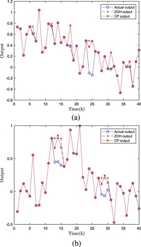
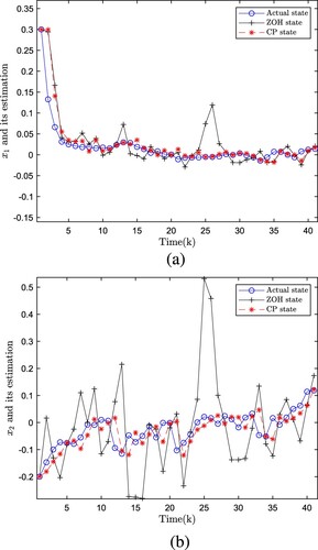
Figure 2 depicts the comparison of the estimated state of the filter based on the CP algorithm, the estimated state of the filter based on the ZOH, and the actual state of the graph. This figure verifies the effectiveness of our algorithm based on CP design. Intuitively, the trend of the three curves in the figure indicates that the method we designed for state estimation performs better. Figure 3 displays the MSE of our designed method, which illustrates that the designed method outperforms the ZOH. To demonstrate the generalization of our designed algorithm, we change the duty cycle parameter to increase an experimental group for comparison. The duty cycle parameters are taken as $d_c^1=0.78$ and $d_c^2=0.87$. It can be observed from Figure 4 that the performance of the CP-based filtering method is effective with both duty cycles.In conclusion, the effectiveness of the designed filtering method has been verified.

Figure 2. Actual states x and their estimates $\hat{x}$ based on CP ($d_c^1=0.8,d_c^2=0.85$). (a) Actual state $x_1$ and its estimate ${\hat{x}}_1$. and (b) Actual state $x_2$ and its estimate ${\hat{x}}_2$.

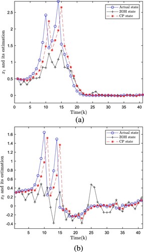
Figure 3. MSE on states based on ZOH and CP($d_c^1=0.8,d_c^2=0.85$). (a) MSE on state $x_1$ based on ZOH and CP. and (b) MSE on state $x_2$ based on ZOH and CP.

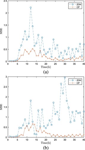
Figure 4. Actual states and their estimates based on CP ($d_c^1=0.78,d_c^2=0.87$). (a) Actual state $x_1$ and its estimate ${\hat{x}}_1$. and (b) Actual state $x_2$ and its estimate ${\hat{x}}_2$.

So far, the simulation results show that the designed CP-based recursive filtering scheme is effective for time-varying nonlinear systems under DCS. Therefore, the research content of this paper is of positive importance for theoretical research and engineering applications.

5. Conclusions

In this paper, we study the filtering problem of sensor-saturated nonlinear systems and propose a CP-based recursive filtering method under DCS. Then, the filter gain that minimizes the upper bound on the error covariance is obtained. In addition, a sufficient condition has been given to ensure that the upper bound on the filtering error covariance is bounded. Finally, the effectiveness of the filtering scheme is verified by a simulation example. In the future, we will employ the designed filtering algorithm for a variety of other scientific and engineering applications, including but not limited to transmission line fault diagnosis (Shakiba et al., 2022), microseismic occasion location (Gao et al., 2021), data denoising (X. Li et al., 2022), image confirmation (Quan et al., 2021), object tracking (Geng et al., 2022) and image registration (Chen et al., 2020).

Disclosure statement

No potential conflict of interest was reported by the author(s).

Additional information

Funding

This work was supported in part by the Young Top Talents Fund in the School of Electrical Information Engineering of Northeast Petroleum University.

References

- Alsaadi, F. E., Liu, Y., & Alharbi, N. S. (2022). Design of robust H∞ state estimator for delayed polytopic uncertain genetic regulatory networks: Dealing with finite-time boundedness. Neurocomputing, 497, 170–181. https://doi.org/10.1016/j.neucom.2022.05.018
- Bag, S., Kumar, S. K., & Tiwari, M. K. (2019). An efficient recommendation generation using relevant Jaccard similarity. Information Sciences, 483, 53–64. https://doi.org/10.1016/j.ins.2019.01.023
- Benesty, J., Chen, J., Huang, Y., & Cohen, I. (2009). Pearson correlation coefficient. Noise Reduction in Speech Processing, 1–4.
- Bobadilla, J., Hernando, A., Ortega, F., & Gutiérrez, A. (2012). Collaborative filtering based on significances. Information Sciences, 185(1), 1–17. https://doi.org/10.1016/j.ins.2011.09.014
- Bu, X., Dong, H., Han, F., Hou, N., & Li, G. (2019). Distributed filtering for time-varying systems over sensor networks with randomly switching topologies under the Round-Robin protocol. Neurocomputing, 346, 58–64. https://doi.org/10.1016/j.neucom.2018.07.087
- Bu, X., Song, J., Huo, F., & Yang, F. (2022). Dynamic event-triggered resilient state estimation for time-varying complex networks with Markovian switching topologies. ISA Transactions, 127, 50–59. https://doi.org/10.1016/j.isatra.2022.05.012
- Chen, Y., He, F., Li, H., Zhang, D., & Wu, Y. (2020). A full migration BBO algorithm with enhanced population quality bounds for multimodal biomedical image registration. Applied Soft Computing, 93, Article 106335. https://doi.org/10.1016/j.asoc.2020.106335
- Gao, H., Han, F., Jiang, B., Dong, H., & Li, G. (2020). Recursive filtering for time-varying systems under duty cycle scheduling based on collaborative prediction. Journal of the Franklin Institute-engineering and Applied Mathematics, 357(17), 13189–13204. https://doi.org/10.1016/j.jfranklin.2020.09.035
- Gao, H., Zhang, M., Hou, N., & Dong, H. (2021). Dynamic-transmission-based recursive filtering algorithm for microseismic event detection under sensor saturations. Measurement, 186, Article 110197. https://doi.org/10.1016/j.measurement.2021.110197
- Geng, S., Zhu, C., Jin, Y., Wang, L., & Tan, H. (2022). Gaze control system for tracking Quasi-1D high-speed moving object in complex background. Systems Science & Control Engineering, 10(1), 367–376. https://doi.org/10.1080/21642583.2022.2063204
- Gu, Y., Hwang, J., He, T., & Du, D. H. C. (2007). usense: A unified asymmetric sensing coverage architecture for wireless sensor networks. In 27th international conference on distributed computing systems (ICDCS '07), Toronto, ON, Canada (p. 8).
- Guo, J., Deng, J., Ran, X., Wang, Y., & Jin, H. (2021). An efficient and accurate recommendation strategy using degree classification criteria for item-based collaborative filtering. Expert Systems with Applications, 164, Article 113756. https://doi.org/10.1016/j.eswa.2020.113756
- Guo, T., Luo, J., Dong, K., & Yang, M. (2019). Locally differentially private item-based collaborative filtering. Information Sciences, 502, 229–246. https://doi.org/10.1016/j.ins.2019.06.021
- Han, F., Wang, Z., Dong, H., Alsaadi, F. E., & Alharbi, K. H. (2022). A local approach to distributed H∞-consensus state estimation over sensor networks under hybrid attacks: Dynamic event-triggered scheme. IEEE Transactions on Signal and Information Processing Over Networks, 8, 556–570. https://doi.org/10.1109/TSIPN.2022.3182273
- Hu, J., Jia, C., Yu, H., & Liu, H. (2022). Dynamic event-triggered state estimation for nonlinear coupled output complex networks subject to innovation constraints. IEEE/CAA Journal of Automatica Sinica, 9(5), 941–944. https://doi.org/10.1109/JAS.2022.105581
- Hu, L. S., Bai, T., Shi, P., & Wu, Z. (2007). Sampled-data control of networked linear control systems. Automatica, 43(5), 903–911. https://doi.org/10.1016/j.automatica.2006.11.015
- Jia, C., Hu, J., Chen, D., Cao, Z., Huang, J., & Tan, H. (2022). Adaptive event-triggered state estimation for a class of stochastic complex networks subject to coding-decoding schemes and missing measurements. Neurocomputing, 494, 297–307. https://doi.org/10.1016/j.neucom.2022.04.096
- Jiang, B., Dong, H., Shen, Y., & Mu, S. (2022). Encoding-decoding-based recursive filtering for fractional-order systems. IEEE/CAA Journal of Automatica Sinica, 9(6), 1103–1106. https://doi.org/10.1109/JAS.2022.105644
- Kommuri, S. K., Defoort, M., Karimi, H. R., & Veluvolu, K. C. (2016). A robust observer-based sensor fault-tolerant control for PMSM in electric vehicles. IEEE Transactions On Industrial Electronics, 63(12), 7671–7681. https://doi.org/10.1109/TIE.2016.2590993
- Kumar, A., Zhao, M., Wong, K. J., Guan, Y. L., & Chong, P. H. J. (2018). A comprehensive study of IoT and WSN MAC protocols: Research issues, challenges and opportunities. IEEE Access, 6, 76228–76262. https://doi.org/10.1109/Access.6287639
- Kundur, D., & Hatzinakos, D. (1998). A novel blind deconvolution scheme for image restoration using recursive filtering. IEEE Transactions on Signal Processing, 46(2), 375–390. https://doi.org/10.1109/78.655423
- Li, M., Liang, J., & Wang, F. (2022). Robust set-membership filtering for two-dimensional systems with sensor saturation under the Round-Robin protocol. International Journal of Systems Science, 53(13), 2773–2785. https://doi.org/10.1080/00207721.2022.2049918
- Li, W., Sun, J., Jia, Y., Du, J., & Fu, X. (2017). Variance-constrained state estimation for nonlinear complex networks with uncertain coupling strength. Digital Signal Processing, 67, 107–115. https://doi.org/10.1016/j.dsp.2017.02.014
- Li, X., Feng, S., Hou, N., Wang, R., Li, H., Gao, M., & Li, S. (2022). Surface microseismic data denoising based on sparse autoencoder and Kalman filter. Systems Science & Control Engineering, 10(1), 616–628.
- Li, Z., Hu, J., & Li, J. (2021). Distributed filtering for delayed nonlinear system with random sensor saturation: A dynamic event-triggered approach. Systems Science & Control Engineering, 9(1), 440–454. https://doi.org/10.1080/21642583.2021.1919935
- Liu, D., & Ye, D. (2020). Pinning-observer-based secure synchronization control for complex dynamical networks subject to DoS attacks. IEEE Transactions on Circuits and Systems I: Regular Papers, 67(12), 5394–5404. https://doi.org/10.1109/TCSI.8919
- Liu, J., Yin, T., Shen, M., Xie, X., & Cao, J. (2020). State estimation for cyber-physical systems with limited communication resources, sensor saturation and denial-of-service attacks. ISA Transactions, 104, 101–114. https://doi.org/10.1016/j.isatra.2018.12.032
- Liu, L., Ma, L., Zhang, J., & Bo, Y. (2021). Distributed non-fragile set-membership filtering for nonlinear systems under fading channels and bias injection attacks. International Journal of Systems Science, 52(6), 1192–1205. https://doi.org/10.1080/00207721.2021.1872118
- Liu, S., Wang, Z., Wei, G., & Li, M. (2020). Distributed set-membership filtering for multirate systems under the round-robin scheduling over sensor networks. IEEE Transactions on Cybernetics, 50(5), 1910–1920. https://doi.org/10.1109/TCYB.6221036
- Nguyen, H. V., & Bai, L. (2011). Cosine similarity metric learning for face verification. In Computer vision-ACCV 2010: 10th Asian conference on computer vision, Queenstowm, New Zealand (pp. 709–720). Springer.
- Quan, Q., He, F., & Li, H. (2021). A multi-phase blending method with incremental intensity for training detection networks. The Visual Computer, 37(2), 245–259. https://doi.org/10.1007/s00371-020-01796-7
- Sedgwick, P. (2012). Pearson's correlation coefficient. BMJ, 345, Article e4483. https://doi.org/10.1136/bmj.e4483
- Seifoddini, H., & Djassemi, M. (1991). The production data-based similarity coefficient versus Jaccard's similarity coefficient. Computers & Industrial Engineering, 21(1–4), 263–266. https://doi.org/10.1016/0360-8352(91)90099-R
- Shakiba, F. M., Shojaee, M., Azizi, S. M., & Zhou, M. (2022). Real-time sensing and fault diagnosis for transmission lines. International Journal of Network Dynamics and Intelligence, 1(1), 36–47. https://doi.org/10.53941/ijndi0101004
- Shen, B., Wang, Z., Wang, D., & Li, Q. (2020). State-saturated recursive filter design for stochastic time-varying nonlinear complex networks under deception attacks. IEEE Transactions on Neural Networks and Learning Systems, 31(10), 3788–3800. https://doi.org/10.1109/TNNLS.5962385
- Sheugh, L., & Alizadeh, S. H. (2015). A note on Pearson correlation coefficient as a metric of similarity in recommender system. In 2015 AI & Robotics (IRANOPEN) (pp. 1–6).
- Su, X., & Khoshgoftaar, T. M. (2009). A survey of collaborative filtering techniques. Advanced Artificial Intelligence, 2009, 1–19. https://doi.org/10.1155/2009/421425
- Sun, Y., Tian, X., & Wei, G. (2022). Finite-time distributed resilient state estimation subject to hybrid cyber-attacks: A new dynamic event-triggered case. International Journal of Systems Science, 53(13), 2832–2844. https://doi.org/10.1080/00207721.2022.2083256
- Suo, J., Li, N., & Li, Q. (2021). Event-triggered H∞ state estimation for discrete-time delayed switched stochastic neural networks with persistent dwell-time switching regularities and sensor saturations. Neurocomputing, 455, 297–307. https://doi.org/10.1016/j.neucom.2021.01.131
- Tao, H., Tan, H., Chen, Q., Liu, H., & Hu, J. (2022). H∞ state estimation for memristive neural networks with randomly occurring DoS attacks. Systems Science & Control Engineering, 10(1), 154–165. https://doi.org/10.1080/21642583.2022.2048322
- Theodor, Y., & Shaked, U. (1996). Robust discrete-time minimum-variance fifiltering. IEEE Transactions on Signal Processing, 44(2), 181–189. https://doi.org/10.1109/78.485915
- Tripathi, Y., Prakash, A., & Tripathi, R. (2022). A novel slot scheduling technique for duty-cycle based data transmission for wireless sensor network. Digital Communications and Networks, 8(3), 351–358. https://doi.org/10.1016/j.dcan.2022.01.006
- Wang, D., Lu, H., & Bo, C. (2015). Visual tracking via weighted local cosine similarity. IEEE Transactions on Cybernetics, 45(9), 1838–1850. https://doi.org/10.1109/TCYB.2014.2360924
- Wang, F., & Liu, J. (2012). On reliable broadcast in low duty-cycle wireless sensor networks. IEEE Transactions on Mobile Computing, 11(5), 767–779. https://doi.org/10.1109/TMC.2011.94
- Yang, B., Lei, Y., Liu, J., & Li, W. (2017). Social collaborative filtering by trust. IEEE Transactions on Pattern Analysis and Machine Intelligence, 39(8), 1633–1647. https://doi.org/10.1109/TPAMI.2016.2605085
- Yao, F., Ding, Y., Hong, S., & Yang, S.-H. (2022). A survey on evolved LoRa-based communication technologies for emerging internet of things applications. International Journal of Network Dynamics and Intelligence, 1(1), 4–19. https://doi.org/10.53941/ijndi0101002
- Yoo, H., Shim, M., & Kim, D. (2012). Dynamic duty-cycle scheduling schemes for energy-harvesting wireless sensor networks. IEEE Communications Letters, 16(2), 202–204. https://doi.org/10.1109/LCOMM.2011.120211.111501
- Young, I. T., & L. J. Van. Vliet (1995). Recursive implementation of the Gaussian filter. Signal Processing, 44(2), 139–151. https://doi.org/10.1016/0165-1684(95)00020-E
- Yu, K., Schwaighofer, A., Tresp, V., Xu, X., & Kriegel, H. P. (2004). Probabilistic memory-based collaborative filtering. IEEE Transactions on Knowledge and Data Engineering, 16(1), 56–69. https://doi.org/10.1109/TKDE.2004.1264816
- Zhang, H., Zhang, X., & Bu, R. (2021). Active disturbance rejection control of ship course keeping based on nonlinear feedback and ZOH component. Ocean Engineering, 233, Article 109136. https://doi.org/10.1016/j.oceaneng.2021.109136
- Zhang, W. A., Yu, L., & Feng, G. (2011). Optimal linear estimation for networked systems with communication constraints. Automatica, 47(9), 1992–2000. https://doi.org/10.1016/j.automatica.2011.05.020
- Zhao, Y., He, X., Ma, L., & Liu, H. (2022). Unbiasedness-constrained least squares state estimation for time-varying systems with missing measurements under round-robin protocol. International Journal of Systems Science, 53(9), 1925–1941. https://doi.org/10.1080/00207721.2022.2031338
- Zou, L., Wang, Z., Geng, H., & Liu, X. (2021). Set-membership filtering subject to impulsive measurement outliers: A recursive algorithm. IEEE/CAA Journal of Automatica Sinica, 8(2), 377–388. https://doi.org/10.1109/JAS.6570654