A novel adaptive PID controller with new seesaw algorithms using alternative derivatives

ABSTRACT

The $\mathrm{PID}$ controller is present in at least 90% of industrial applications due to its simplicity and robustness to control linear and non-linear systems. Its main drawbacks include difficulty in achieving proper gains tuning for complex systems and lack of adaptability attributed to its fixed gains when system dynamics change. Despite the emergence of promising controllers like Neural Networks, Fuzzy Logic, Sliding Modes, or Genetic Algorithms, diverse research efforts focus on using these to improve the $\mathrm{PID}$ rather than replacing it, aiming for either ideal fixed gains or adaptive gains. Nevertheless, while some require system models, training data, rules establishment, extensive iterations, and demanding computational resources, the $\mathrm{PID}$ and the novel $\mathrm{APID}$ controller do not. The new seesaw algorithms propose alternative behaviours based on the current error and its derivative, which are dynamic parameters that change over time. These behaviours can be inserted into the $\mathrm{PID}$ to imbue it with adaptive characteristics, achieving adaptive $\mathrm{PID}$ ($\mathrm{SeesawAPID}$) controllers with faster signal rise and stabilization times, reduction of the maximum peak, and less error accumulation compared to conventional $\mathrm{PID}$.

KEYWORDS:

• Seesaw algorithms
• alternative derivatives
• adaptive PID control
• control algorithms
• adaptive control
• PID control

1. Introduction

The need for adaptability in controllers arises due to the changes experienced by systems. Consider the Segway as an example. During operation, it encounters various changes such as users with distinct physical attributes or changing payloads, diverse terrains, and weather conditions, all affecting its performance. Even natural wear and tear of components alters the system and affects the controller's performance. These examples can be extended to many other controlled systems.

The $\mathrm{PID}$ controller is widely used in the industry (Åström & Hägglund, 2001), comprising 90-95% of control applications. including modern applications such as autonomous cars, unmanned aerial vehicles, and autonomous robots (Díaz-Rodríguez et al., 2019). This controller, with its three terms, is employed to achieve system stability and to decrease steady-state error (Johnson et al., 2005), addressing both transient and steady-state responses. Due to its structure, easy implementation, and maintenance (Åström & Hägglund, 2001), it offers simple and efficient solutions to many control problems. However, each term of the $\mathrm{PID}$ has a fixed gain without dynamics, making it unresponsive to changes. As a result, proper gain tuning is crucial for optimal performance (Ang et al., 2005; Johnson et al., 2005). However, even when tuned to withstand some variations, the $\mathrm{PID}$ lacks adaptability.

Adaptive features in control algorithms aim to improve controller performance in response to system changes. This has led research efforts to combine PID controllers with other strategies (Swarnkar et al., 2014), either to achieve optimal PID gain tuning or to develop adaptive PID controllers (APIDs) with dynamic PID gains.

Noordin et al. (2023) developed an $\mathrm{APID}$ that combines Sliding Mode Control ($\mathrm{SMC}$) and Fuzzy Logic ($\mathrm{FL}$) for a drone's altitude control, aiming for adaptability to variable loads, achieving a 46% improvement over the $\mathrm{PID}$. Its complexity involves a sliding surface proposal, parameters and gains tuning rules, and $\mathrm{FL}$ rules to mitigate chattering from $\mathrm{SMC}$. $\mathrm{APID}$ and $\mathrm{FL}$ gains were manually adjusted. Zeng et al. (2012) developed an $\mathrm{APID}$ that combines Neural Networks ($\mathrm{NN}$) and $\mathrm{PID}$ to enhance control against external weather fluctuations in a greenhouse. It involves at least a system model and a Radial Basis Function ($\mathrm{RBF}$) network to identify and tune the $\mathrm{PID}$ parameters. It was compared with an optimized $\mathrm{PID}$ by Genetic Algorithm ($\mathrm{GA}$), an offline tuning that provides fixed gains. $\mathrm{GA}$ requires a mathematical model and multiple iterations involving demanding computational resources. Authors claim that the $\mathrm{APID}$ has better reference tracking and disturbance rejection. However, the $\mathrm{GA}$-optimized $\mathrm{PID}$ shows better quantitative performance. Han et al. combined $\mathrm{NN}$, $\mathrm{GA}$, $\mathrm{FL}$, and $\mathrm{PID}$ to achieve an $\mathrm{APID}$ for vehicle suspension control (Han et al., 2022). Diverse control strategies were employed to adjust the system model through data training and parameter optimization. Also, different approaches were used to estimate a dynamic reference and to design a competent $\mathrm{APID}$ for changing road scenarios. The $\mathrm{APID}$ had remarkable results; still, the $\mathrm{PID}$ controller exhibited adequate performance. Wogi et al. (2022) developed an $\mathrm{APID}$ combining $\mathrm{FL}$ and $\mathrm{PID}$ to control an induction motor. The $\mathrm{APID}$ was compared with a Fuzzy $\mathrm{SMC}$ controller. Both controllers perform very well, although the Fuzzy$\mathrm{SMC}$ is superior. It is worth noting that the $\mathrm{APID}$ required 49 rules for each $\mathrm{PID}$ gain, and the inputs for these rules, which consequently establish the control signal, were the error, $e(t)$, and its derivative, $\mathrm{de}(t)/\mathrm{dt}$, which coincidently are vital for the seesaw algorithms. Many other examples can be mentioned regarding adaptive $\mathrm{PID}$ control (Karanjkar et al., 2014; Khan et al., 2016; Mahmoodabadi & Safi Jahanshahi, 2021; Prabhakar et al., 2019; Wang et al., 2015).

As can be seen, the label ‘adaptive’ has been used to describe controllers that can adjust their control coefficients in real-time to account for system variations (Swarnkar et al., 2014). However, combining two or more controllers can increase complexity in terms of understanding, implementation, and computational demands.

The proposed algorithms can endow $\mathrm{PID}$ controllers with adaptive features, achieving variable gains with dynamic adjustments according to $e(t)$ and $\mathrm{de}(t)/\mathrm{dt}$. These adaptive $\mathrm{PID}$ controllers ($\mathrm{Seesaw}\mathrm{APIDs}$) derived from the new seesaw algorithms, do not require system models, training data, rule establishment, or extensive iterative processes. Since they are based on $\mathrm{PID}$, which is well-documented, their implementation and understanding are relatively straightforward, and excessive processing requirements will not be demanded.

The rest of this article is organized as follows: Section 2 provides a visual explanation of the algorithms. Sections 3 and 4 explore the mathematical aspects of the algorithms and their implementation. Section 5 presents the modelling of an inverted pendulum on a cart (IPC), which serves as our test plant. Section 6 presents the necessary code for programming and incorporating the algorithms into the $\mathrm{PID}$. Section 7 demonstrates the functionality of the algorithms and their implementation into the $\mathrm{PID}$ for controlling two different plants. Section 8 delves into the results. Section 9 outlines future work directions.

2. Graphic approach

Within a control strategy, the derivative of the error, $\mathrm{de}(t)/\mathrm{dt}$, can be understood as an estimation of the future behaviour of a system; in this sense, there is a behaviour inherent in the original slope value, $m_{\mathrm{orig}}$ ($\mathrm{de}(t)/\mathrm{dt}$), of a signal, $(t,e(t))$. Seesaw algorithms keep the current instant, $t$, as a pivot and modify the slope, $m_{\mathrm{orig}}$, that exists in the control strategy ($\mathrm{PID}$ control) using $e(t)$ and $\mathrm{de}(t)/\mathrm{dt}$. The results thereof will give a new slope value, a new alternative slope, $m_{\mathrm{alt}}$ ($d_{\mathrm{alt}}e(t)/\mathrm{dt}$), so that the perpendicularity of $m_{\mathrm{orig}}$ can be manipulated. When $m_{\mathrm{orig}}$ is modified and an alternative derivative, $m_{\mathrm{alt}}$, is generated, alternative behaviour proposals will be created and can be inserted into $\mathrm{PID}$ formulation to make the $\mathrm{PID}$ gains fit to them. This work shows two ways of modifying $m_{\mathrm{orig}}$ from $e(t)$ and $\mathrm{de}(t)/\mathrm{dt}$: the MS and LS seesaw algorithms. The MS seesaw algorithm will speed up the approach toward the set point, $\mathrm{SP}$, and the LS seesaw algorithm will damp the approach toward the $\mathrm{SP}$. Visually, changing from $m_{\mathrm{orig}}$ to $m_{\mathrm{alt}}$ will exhibit a seesaw effect, no matter which algorithm is employed.

2.1. MS seesaw algorithm

From a graphical approach (Figure 1), consider the current instant, $t$, of the output and the original slope, $m_{\mathrm{orig}}$. A point, $A_1$, is generated over $m_{\mathrm{orig}}$. $A_1$ is defined by $V_{\mathrm{om}}\cdot e(t)$. $e(t)$ is the current error and $V_{\mathrm{om}}$ is a magnitude applied over $m_{\mathrm{orig}}$; therefore, $V_{\mathrm{om}}\cdot e(t)$ is $e(t)$'s magnitude variation over $m_{\mathrm{orig}}$.

Figure 1. $m_{\mathrm{alt}}$ generation with MS seesaw algorithm (a) when $V_{\mathrm{om}}\cdot e(t)=1\cdot e(t)$ and $V_{\mathrm{oy}}\cdot e(t)=1\cdot e(t)$; and (b) when $m_{\mathrm{orig}}$ tends to infinity.

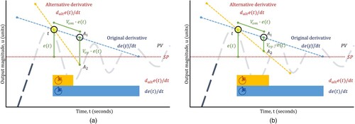
With $A_1$, another point, $A_2$, defined by $V_{\mathrm{oy}}\cdot e(t)$, is generated. $V_{\mathrm{oy}}$ is a magnitude applied over the y-axis; therefore, $V_{\mathrm{oy}}\cdot e(t)$ is $e(t)$'s magnitude variation over the $y$-axis. With $A_2$ and the current instant, $t$, an alternative slope, $m_{\mathrm{alt}}$, which is different from $m_{\mathrm{orig}}$, is generated. $m_{\mathrm{alt}}$ converges to the $\mathrm{SP}$ in less time (Figure 1). The behaviour that $m_{\mathrm{alt}}$ proposes is manipulated with $V_{\mathrm{om}}$ and $V_{\mathrm{oy}}$.

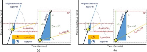
2.2. LS seesaw algorithm

Considering $t$ and $m_{\mathrm{orig}}$, a point, $A_1$ is generated at the intersection of $m_{\mathrm{orig}}$ and the $\mathrm{SP}$. With $A_1$, another point, $A_2$, defined by $V_{\mathrm{pct}}\cdot e(t)$ is generated. $V_{\mathrm{pct}}$ is a percentage magnitude (between 0 and 1) applied over the $y$-axis; therefore, $V_{\mathrm{pct}}\cdot e(t)$ is a percentage variation of $e(t)$'s magnitude on the $y$-axis. With $A_2$, a $m_{\mathrm{alt}}$ value of less than $m_{\mathrm{orig}}$ is generated (Figure 2). The behavior that $m_{\mathrm{alt}}$ proposes is manipulated with $V_{\mathrm{pct}}$.

Figure 2. $m_{\mathrm{alt}}$ generation with LS seesaw algorithm when (a) $V_{\mathrm{pct}}\cdot e(t)=0.9\cdot e(t)$ and when (b) $V_{\mathrm{pct}}\cdot e(t)=0.8\cdot e(t)$.

3. Math formulation: Seesaw algorithms

The procedures of both seesaw algorithms are shown, and for both, the rectangular coordinates $(x_{\mathrm{actual}},y_{\mathrm{actual}})$ of the current instant, $t$, are established – $(t,e(t))$ – and act as a pivot: (1) $P_{\mathrm{actual}}(x_{\mathrm{actual}},y_{\mathrm{actual}})=P_{\mathrm{actual}}(t,e(t)$(1)

3.1. MS seesaw algorithm

The angle ${\theta }_{\mathrm{orig}}$ corresponding to $m_{\mathrm{orig}}$ at $t$ is calculated: (2) $\tan ({\theta }_{\mathrm{orig}})=m_{\mathrm{orig}}\to {\theta }_{\mathrm{orig}}={\tan }^{-1}(m_{\mathrm{orig}})$(2)

A new vector with polar coordinates $(r,\theta )$ is generated; here, $r$ is defined by $V_{\mathrm{om}}\cdot e(t)$ and $\theta$ is defined by ${\theta }_{\mathrm{orig}}$: (3) $(r,\theta )=(V_{\mathrm{om}}\cdot e(t),{\theta }_{\mathrm{orig}})$(3)

Polar coordinates $(V_{\mathrm{om}}\cdot e(t),{\theta }_{\mathrm{orig}})$ are converted to rectangular coordinates $(x_{\mathrm{om}},y_{\mathrm{om}})$: (4) $\begin{array}{rl}{x}_{\mathrm{om}}& =V_{\mathrm{om}}\cdot e(t)\cos ({\theta }_{\mathrm{orig}})\end{array}$(4) (5) $\begin{array}{rl}{y}_{\mathrm{om}}& =V_{\mathrm{om}}\cdot e(t)\sin ({\theta }_{\mathrm{orig}})\end{array}$(5)

Although it presents magnitude, direction, and sense, the vector $(V_{\mathrm{om}}\cdot e(t),{\theta }_{\mathrm{orig}})$ is established to not correspond to the position of the current instant, $(t,e(t))$; the same goes for $(x_{\mathrm{om}},y_{\mathrm{om}})$.

$P_{\mathrm{actual}}(x_{\mathrm{actual}},y_{\mathrm{actual}})$ is added to the rectangular coordinates $(x_{\mathrm{om}},y_{\mathrm{om}})$ to generate a point $P_{\mathrm{alt}1}(x_{\mathrm{alt}1},y_{\mathrm{alt}1})$ over $m_{\mathrm{orig}}$ that is different from $(t,e(t))$: (6) $\begin{array}{rl}& \begin{array}{l}{x}_{\mathrm{alt}1}=x_{\mathrm{om}}+x_{\mathrm{actual}}\\ x_{\mathrm{alt}1}=V_{\mathrm{om}}\cdot e(t)\cos ({\theta }_{\mathrm{orig}})+t\end{array}\end{array}$(6) (7) $\begin{array}{rl}& \begin{array}{l}{y}_{\mathrm{alt}1}=y_{\mathrm{om}}+y_{\mathrm{actual}}\\ y_{\mathrm{alt}1}=V_{\mathrm{om}}\cdot e(t)\sin ({\theta }_{\mathrm{orig}})+e(t)\end{array}\end{array}$(7)

A new point, $P_{\mathrm{alt}2}$, is generated from $P_{\mathrm{alt}1}$ by the alteration of the $y_{\mathrm{alt}1}$ coordinate. This alteration is achieved with the addition or subtraction of $V_{\mathrm{oy}}\cdot e(t)$ according to $(t,e(t))$. If $e(t)$ is negative, an addition must be made; if it is positive, a subtraction must be made. $e(t)$ is established to be negative when $(t,e(t))$ exceeds the $\mathrm{SP}$, and $e(t)$ is positive if, at that instant, $(t,e(t))$ is below the $\mathrm{SP}$.

In the case of addition, when $e(t)$ is negative, consider $P_{\mathrm{alt}2}$ to be. (8) $\begin{array}{rl}& x_{\mathrm{alt}2}=x_{\mathrm{alt}1}=V_{\mathrm{om}}\cdot e(t)\cos ({\theta }_{\mathrm{orig}})+t\end{array}$(8) (9) $\begin{array}{r}\begin{array}{rl}& y_{\mathrm{alt}2}=y_{\mathrm{alt}1}+V_{\mathrm{oy}}\cdot e(t)\\ & y_{\mathrm{alt}2}=V_{\mathrm{om}}\cdot e(t)\sin ({\theta }_{\mathrm{orig}})+e(t)+V_{\mathrm{oy}}\cdot e(t)\end{array}\end{array}$(9)

To generate $m_{\mathrm{alt}}$ in the case of addition, the slope between points $P_{\mathrm{actual}}$ and $P_{\mathrm{alt}2}$ is calculated: (10) $\begin{array}{rl}& m_{\mathrm{alt}}=\frac{y_2-y_1}{x_2-x_1}=\frac{y_{\mathrm{alt}2}-y_{\mathrm{actual}}}{x_{\mathrm{alt}2}-x_{\mathrm{actual}}}\\ & m_{\mathrm{alt}}=\frac{V_{\mathrm{om}}\cdot e(t)\sin ({\theta }_{\mathrm{orig}})e(t)+V_{\mathrm{oy}}\cdot e(t)-e(t)}{V_{\mathrm{om}}\cdot e(t)\cos ({\theta }_{\mathrm{orig}})+t-t}\\ & m_{\mathrm{alt}}=m_{\mathrm{orig}}+\frac{V_{\mathrm{oy}}}{V_{\mathrm{om}}}\cdot \frac{1}{\cos ({\theta }_{\mathrm{orig}})}\end{array}$(10)

In the case of subtraction, when $e(t)$ is positive, consider $P_{\mathrm{alt}2}$ as (11) $\begin{array}{rl}{x}_{\mathrm{alt}2}& =x_{\mathrm{alt}1}=V_{\mathrm{om}}\cdot e(t)\cos ({\theta }_{\mathrm{orig}})+t\end{array}$(11) (12) $\begin{array}{r}\begin{array}{rl}{y}_{\mathrm{alt}2}& =y_{\mathrm{alt}1}-V_{\mathrm{oy}}\cdot e(t)\\ y_{\mathrm{alt}2}& =V_{\mathrm{om}}\cdot e(t)\sin ({\theta }_{\mathrm{orig}})+e(t)-V_{\mathrm{oy}}\cdot e(t)\end{array}\end{array}$(12)

To generate $m_{\mathrm{alt}}$ in the case of subtraction, the slope between points $P_{\mathrm{actual}}$ and $P_{\mathrm{alt}2}$ is calculated: (13) $\begin{array}{rl}{m}_{\mathrm{alt}}& =\frac{y_2-y_1}{x_2-x_1}=\frac{y_{\mathrm{alt}2}-y_{\mathrm{actual}}}{x_{\mathrm{alt}2}-x_{\mathrm{actual}}}\\ m_{\mathrm{alt}}& =\frac{V_{\mathrm{om}}\cdot e(t)\sin ({\theta }_{\mathrm{orig}})+e(t)-V_{\mathrm{oy}}\cdot e(t)-e(t)}{V_{\mathrm{om}}\cdot e(t)\cos ({\theta }_{\mathrm{orig}})+t-t}\\ m_{\mathrm{alt}}& =m_{\mathrm{orig}}-\frac{V_{\mathrm{oy}}}{V_{\mathrm{om}}}\cdot \frac{1}{\cos ({\theta }_{\mathrm{orig}})}\end{array}$(13)

3.2. LS seesaw algorithm

The angle ${\theta }_{\mathrm{orig}}$ corresponding to the $m_{\mathrm{orig}}$ of $t$ is calculated: (14) $\tan ({\theta }_{\mathrm{orig}})=m_{\mathrm{orig}}\to {\theta }_{\mathrm{orig}}={\tan }^{-1}(m_{\mathrm{orig}})$(14)

The rectangular coordinates of the intersection are set to be $(x_{\mathrm{cross}},y_{\mathrm{cross}})$: (15) $P_{\mathrm{cross}}(x_{\mathrm{cross}},y_{\mathrm{cross}})=P_{\mathrm{cross}}(x_{\mathrm{cross}},\mathrm{SP})$(15)

The $x$-coordinate of the intersection between $m_{\mathrm{orig}}$ and $\mathrm{SP}$ is calculated: (16) $\begin{array}{rl}{m}_{\mathrm{orig}}& =\frac{y_{\mathrm{cross}}-y_{\mathrm{actual}}}{x_{\mathrm{cross}}-x_{\mathrm{actual}}}=\frac{\mathrm{SP}-e(t)}{x_{\mathrm{cross}}-t}\end{array}$(16) (17) $\begin{array}{rl}{x}_{\mathrm{cross}}& =\frac{\mathrm{SP}-e(t)}{m_{\mathrm{orig}}}+t\end{array}$(17)

A new point, $P_{\mathrm{alt}1}$, is generated from $P_{\mathrm{cross}}$, altering $y_{\mathrm{cross}}$: (18) $P_{\mathrm{alt}1}(x_{\mathrm{alt}1},y_{\mathrm{alt}1})$(18) $y_{\mathrm{cross}}$ alteration is achieved with the addition of $V_{\mathrm{pct}}\cdot e(t)$. The coordinates $(x_{\mathrm{alt}1},y_{\mathrm{alt}1})$ are defined as (19) $\begin{array}{rl}{x}_{\mathrm{alt}1}& =x_{\mathrm{cross}}=\frac{\mathrm{SP}-e(t)}{m_{\mathrm{orig}}}+t\end{array}$(19) (20) $\begin{array}{rl}{y}_{\mathrm{alt}1}& =y_{\mathrm{cross}}+V_{\mathrm{pct}}\cdot e(t)=\mathrm{SP}+V_{\mathrm{pct}}\cdot e(t)\end{array}$(20)

Point $P_{\mathrm{alt}1}$ can be rewritten as (18) $P_{\mathrm{alt}1}(x_{\mathrm{cross}},y_{\mathrm{cross}}+V_{\mathrm{pct}}\cdot e(t))$(18)

To generate $m_{\mathrm{alt}}$, the slope between points $P_{\mathrm{actual}}$ and $P_{\mathrm{alt}1}$ is calculated: (21) $\begin{array}{rl}{m}_{\mathrm{alt}}& =\frac{y_{\mathrm{alt}1}-y_{\mathrm{actual}}}{x_{\mathrm{alt}1}-x_{\mathrm{actual}}}=\frac{\mathrm{SP}+(V_{\mathrm{pct}}\cdot e(t))-e(t)}{\frac{\mathrm{SP}-e(t)}{m_{\mathrm{orig}}}+t-t}\\ m_{\mathrm{alt}}& =m_{\mathrm{orig}}\left(\frac{\mathrm{SP}+e(t)(V_{\mathrm{pct}}-1)}{\mathrm{SP}-e(t)}\right)\end{array}$(21)

4. Math formulation: $\mathrm{Seesaw}\mathrm{APID}$ control

4.1. Alternative $k_P$ $({k_P}_{\mathrm{alt}})$

$\mathrm{PID}$ control (textbook $\mathrm{PID}$) is used as the foundation (Johnson et al., 2005): (22) $\begin{array}{rl}\mathrm{CO}& =P+I+D\\ \mathrm{CO}& =k_P\cdot e(t)+k_I{\int }_0^{t}e(t)\mathrm{dt}+k_D\frac{\mathrm{de}(t)}{\mathrm{dt}}\\ \mathrm{CO}& =k_P\cdot e(t)+\frac{k_P}{{\tau }_I}{\int }_0^{t}e(t)\mathrm{dt}+k_P\cdot {\tau }_D\frac{\mathrm{de}(t)}{\mathrm{dt}}\\ \mathrm{CO}& =k_P\cdot e(t)+\frac{k_P}{{\tau }_I}{\int }_0^{t}e(t)\mathrm{dt}+k_P\cdot {\tau }_D{m}_{\mathrm{orig}}\end{array}$(22) where $\mathrm{CO}$ is the controller output, $e(t)$ is the error $(\mathrm{SP}\text{--}\mathrm{PV})$, $\mathrm{SP}$ is the set point, $\mathrm{PV}$ is the measured process variable $y(t)$, $k_P$ is the proportional gain, $k_I$ is the integral gain, $k_D$ is the derivative gain, ${\tau }_I$ is the integral time, and ${\tau }_D$ is the derivative time. All of these are known values.

As shown, it is possible to propose $m_{\mathrm{alt}}$ using $m_{\mathrm{orig}}$ and $e(t)$: (23) $m_{\mathrm{alt}}=\frac{d_{\mathrm{alt}}e(t)}{\mathrm{dt}}$(23)

Once $m_{\mathrm{alt}}$ is generated, only the $D$ term from the $\mathrm{PID}$ is considered (Eq. 2(2) $\tan ({\theta }_{\mathrm{orig}})=m_{\mathrm{orig}}\to {\theta }_{\mathrm{orig}}={\tan }^{-1}(m_{\mathrm{orig}})$(2) 2): (24) $D=k_P\cdot {\tau }_D{m}_{\mathrm{orig}}$(24)

$m_{\mathrm{orig}}$ from Equation (24) is replaced with $m_{\mathrm{alt}}$ from Equation (23): (25) $D=k_P\cdot {\tau }_D{m}_{\mathrm{alt}}\to k_P\cdot {\tau }_D{m}_{\mathrm{alt}}=D_{\mathrm{alt}}$(25) where $D_{\mathrm{alt}}$ corresponds to a desired behaviour, and the $D_{\mathrm{alt}}$ value acts as a reference target.

$k_P$ from Equation (24) is isolated as an incognita, and $D$ is replaced with the value of $D_{\mathrm{alt}}$ from Equation (25). This calculation results in an alternative gain, ${k_P}_{\mathrm{alt}}$: (26) $k_P=\frac{D}{{\tau }_D{\text{m}}_{\text{orig}}}\to \frac{D_{\mathrm{alt}}}{{\tau }_D{\text{m}}_{\text{orig}}}={k_P}_{\mathrm{alt}-i}$(26)

Equation (26) was developed: (27) ${k_P}_{\mathrm{alt}-i}=\frac{D_{\mathrm{alt}}}{{\tau }_D{m}_{\mathrm{orig}}}=\frac{k_P\cdot {\tau }_D{m}_{\mathrm{orig}}}{{\tau }_D{m}_{\mathrm{orig}}}=k_P\frac{m_{\mathrm{alt}}}{m_{\mathrm{orig}}}$(27) ${k_P}_{\mathrm{alt}-i}$ varies relative to $e(t)$ and $m_{\mathrm{orig}}$ ($\mathrm{de}(t)/\mathrm{dt}$), which are dynamic values; ${k_P}_{\mathrm{alt}-i}$ adapts to changes, but exhibits indeterminacy when $m_{\mathrm{orig}}=0$ and nullity when $m_{\mathrm{alt}}=0$. To avoid indeterminacy, a number, $\epsilon$, is added to the denominator, thereby creating an applicable alternative gain, ${k_P}_{\mathrm{alt}}$: (28) ${k_P}_{\mathrm{alt}}=\mathrm{\Lambda }\cdot k_P\frac{m_{\mathrm{alt}}}{m_{\mathrm{orig}}+\epsilon }$(28)

4.2. Adaptive $k_P$ $({k_P}_{\mathrm{Adapt}})$

As ${k_P}_{\mathrm{alt}}$ is a dynamic value, eventually, $m_{\mathrm{alt}}=0$ and, consequently, ${k_P}_{\mathrm{alt}}=0$, so, when nullified, the ${k_P}_{\mathrm{alt}}$ gain cannot support control by itself. To avoid nullification and preserve the adaptive dynamics, ${k_P}_{\mathrm{alt}}$ is added to $k_P$. The sum of $k_P$ and ${k_P}_{\mathrm{alt}}$ forms an adaptive gain, ${k_P}_{\mathrm{Adapt}}$; however, adding ${k_P}_{\mathrm{alt}}$ to $k_P$ might lead to instability. To avoid instability, a boundary called $\mathrm{\Lambda }$ is assigned to ${k_P}_{\mathrm{alt}}$ as a scale factor: (29) ${k_P}_{\mathrm{Adapt}}=k_P+{k_P}_{\mathrm{alt}}=k_P\left(1+\frac{\mathrm{\Lambda }\cdot m_{\mathrm{alt}}}{m_{\mathrm{orig}}+\epsilon }\right)$(29)

4.3. Adaptive $\mathrm{PID}$ gains

${k_P}_{\mathrm{Adapt}}$ replaces $k_P$ in the $\mathrm{PID}$ formula. The bounding $\mathrm{\Lambda }$ is used individually in each term, with ${\mathrm{\Lambda }}_P$, ${\mathrm{\Lambda }}_I$, and ${\mathrm{\Lambda }}_D$: (22) $\begin{array}{rl}\mathrm{CO}& =P+I+D\end{array}$(22) (30) $\begin{array}{rl}P& =k_P\cdot e(t)\to {k_P}_{\mathrm{Adapt}}\cdot e(t)=P_{\mathrm{Adapt}}\\ & =k_P\left(1+\frac{{\mathrm{\Lambda }}_P\cdot m_{\mathrm{alt}}}{m_{\mathrm{orig}}+\epsilon }\right)\cdot e(t)\\ P_{\mathrm{Adapt}}& =k_{P_{\mathrm{Adapt}}}\cdot e(t)\end{array}$(30) (31) $\begin{array}{rl}I& =\frac{k_P}{{\tau }_I}{\int }_0^{t}e(t)\mathrm{dt}\to \frac{{k_P}_{\mathrm{Adapt}}}{{\tau }_I}{\int }_0^{t}e(t)\mathrm{dt}\\ & =I_{\mathrm{Adapt}}=\frac{k_P\left(1+\frac{{\mathrm{\Lambda }}_I\cdot m_{\mathrm{alt}}}{m_{\mathrm{orig}}+\epsilon }\right)}{{\tau }_i}{\int }_0^{t}e(t)\mathrm{dt}\\ I_{\mathrm{Adapt}}& =k_{I_{\mathrm{Adapt}}}{\int }_0^{t}e(t)\mathrm{dt}\end{array}$(31) (32) $\begin{array}{rl}D& =k_P\cdot {\tau }_D{m}_{\mathrm{orig}}\to {k_P}_{\mathrm{Adapt}}\cdot {\tau }_D{m}_{\mathrm{orig}}=D_{\mathrm{Adapt}}\\ & =k_P\left(1+\frac{{\mathrm{\Lambda }}_D\cdot m_{\mathrm{alt}}}{m_{\mathrm{orig}}+\epsilon }\right)\cdot {\tau }_D\frac{\mathrm{de}(t)}{\mathrm{dt}}\\ D_{\mathrm{Adapt}}& =k_{D_{\mathrm{Adapt}}}\frac{\mathrm{de}(t)}{\mathrm{dt}}\end{array}$(32)

An adaptive $\mathrm{PID}$ or $\mathrm{Seesaw}\mathrm{APID}$ controller is obtained: (33) $\mathrm{Seesaw}\mathrm{APID}=C{O}_{\mathrm{Adapt}}=P_{\mathrm{Adapt}}+I_{\mathrm{Adapt}}+D_{\mathrm{Adapt}}$(33)

5. Test plant

Figure 3 shows a diagram of an IPC.

Figure 3. IPC.

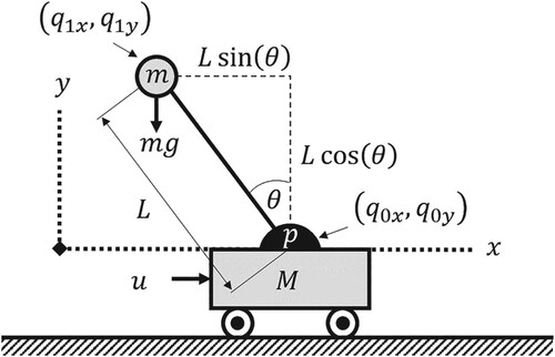
Here, $M$ is the cart's mass, $m$ is the pendulum's mass, $p$ is the pivot, $L$ is the pendulum's length, $x$ is the horizontal axis, $u$ is the driving force, and $\theta$ is the angle from the vertical $(y)$. The position of $M$ is defined by $q_0$, and the position of $m$ is defined by $q_1$. The system and modelling are based on cited references (Prasad et al., 2011; Prasad et al., 2012; Prasad et al., 2014).

$\ddot{x}$ and $\ddot{\theta }$ are obtained: (34) $\begin{array}{rl}\ddot{x}& =\frac{u+\mathrm{mL}{\dot{\theta }}^2\sin (\theta )-\mathrm{mgcos}(\theta )\sin (\theta )}{M+m{\sin }^2(\theta )}\end{array}$(34) (35) $\begin{array}{rl}\ddot{\theta }& =\frac{-\mathrm{ucos}(\theta )-\mathrm{mL}{\dot{\theta }}^2\sin (\theta )\cos (\theta )+(m+M)\mathrm{gsin}(\theta )}{\mathrm{ML}+\mathrm{mL}{\sin }^2(\theta )}\end{array}$(35)

A change in variables is made and the corresponding derivatives are obtained: (36) $\begin{array}{rl}{\dot{x}}_1& =x_2\to \mathrm{Cart}{}^{\mathrm{\prime }}s\mathrm{velocity}\end{array}$(36) (37) $\begin{array}{rl}{\dot{x}}_2& ={\ddot{x}}_2=\ddot{x}\to \mathrm{Cart}{}^{\mathrm{\prime }}s\mathrm{acceleration}\end{array}$(37) (38) $\begin{array}{rl}{\dot{x}}_3& =x_4\to \mathrm{Pendulum}{}^{\mathrm{\prime }}s\mathrm{angular}\mathrm{velocity}\end{array}$(38) (39) $\begin{array}{rl}{\dot{x}}_4& =\ddot{\theta }\to \mathrm{Pendulum}{}^{\mathrm{\prime }}s\mathrm{angular}\mathrm{acceleration}\end{array}$(39)

The variable change is completed: (40) $\begin{array}{rl}{\dot{x}}_2& =\frac{u+\mathrm{mL}{x_4}^2\sin (x_3)-\mathrm{mgcos}(x_3)\sin (x_3)}{M+m{\sin }^2(x_3)}\end{array}$(40) (41) $\begin{array}{rl}{\dot{x}}_4& =\frac{\begin{array}{c}-\mathrm{ucos}(x_3)-\mathrm{mL}{x_4}^2\sin (x_3)\cos (x_3)\\ +(m+M)\mathrm{gsin}(x_3)\end{array}}{\mathrm{ML}+\mathrm{mL}{\sin }^2(x_3)}\end{array}$(41)

6. Programming

In practice, $m_{\mathrm{orig}}$ can be replaced with the derivative of the negative process variable: $-\frac{\mathrm{dPV}(t)}{\mathrm{dt}}$. It allowed us to avoid a phenomenon known as derivative kick (Johnson et al., 2005). Mathematically, since $\mathrm{SP}$ is constant, its derivative is zero. Considering $e(t)=\mathrm{SP}-\mathrm{PV}$, derivation proceeds: (42) $\frac{\mathrm{de}(t)}{\mathrm{dt}}=\frac{\mathrm{dSP}}{\mathrm{dt}}-\frac{\mathrm{dPV}}{\mathrm{dt}}\to \frac{\mathrm{de}(t)}{\mathrm{dt}}=0-\frac{\mathrm{dPV}}{\mathrm{dt}}$(42) To keep track of the already presented theory, $m_{\mathrm{orig}}$ will be used instead of $-\frac{\mathrm{dPV}(t)}{\mathrm{dt}}$ for all of the following codes.

6.1. MS seesaw algorithm code

The following code must be implemented to increase the slope when the signal is convergent to the $\mathrm{SP}$:

If

Condition: $e(t)>0$ & $m_{\mathrm{orig}}<0$ %positive error.

Action: $m_{\mathrm{orig}}-(V_{\mathrm{oy}}/V_{\mathrm{om}})\cdot (1/\cos ({\tan }^{-1}(m_{\mathrm{orig}})))$

Output: $m_{\mathrm{alt}}$

Else If

Condition: $e(t)<0$ & $m_{\mathrm{orig}}>0$ %negative error.

Action: $m_{\mathrm{orig}}+(V_{\mathrm{oy}}/V_{\mathrm{om}})\cdot (1/\cos ({\tan }^{-1}(m_{\mathrm{orig}})))$

Output: $m_{\mathrm{alt}}$

Else

Action: $m_{\mathrm{orig}}$

Output: $m_{\mathrm{orig}}$

6.2. LS seesaw algorithm code

The following code must be implemented to decrease the slope when the signal is convergent to the $\mathrm{SP}$:

If

Condition: $e(t)>0$ & $m_{\mathrm{orig}}<0$%positive error.

Action: $m_{\mathrm{orig}}(\mathrm{SP}+e(t)(V_{\mathrm{pct}}-1)/\mathrm{SP}-e(t))$

Output: $m_{\mathrm{alt}}$

Else If

Condition: $e(t)<0$ & $m_{\mathrm{orig}}>0$ %negative error.

Action: $m_{\mathrm{orig}}(\mathrm{SP}+e(t)(V_{\mathrm{pct}}-1)/\mathrm{SP}-e(t))$

Output: $m_{\mathrm{alt}}$

Else

Action: $m_{\mathrm{orig}}$

Output: $m_{\mathrm{orig}}$

6.3. Seesaw algorithms code for $\mathrm{PID}$ control

The previous codes are suitable for the visualization of the calculation of $m_{\mathrm{alt}}$. However, when the seesaw algorithms are applied in the $\mathrm{PID}$, the very nature of each algorithm must be considered, such as whether it is desired to act at all times of the convergent signal toward the $\mathrm{SP}$ or in specific intervals. If specific intervals are chosen, it is necessary (when programming) to change the ‘If and else Conditions’ when calculating $m_{\mathrm{alt}}$. For the plants evaluated in this article, a change in the ‘If and else Conditions’ – ($e(t)>0.025$ & $m_{\mathrm{orig}}<0$ and $e(t)<-0.025$ & $m_{\mathrm{orig}}>0$) – was performed in the MS seesaw algorithm code. Both algorithms can be ‘Conditions’ modified for the calculation of $m_{\mathrm{alt}}$ if appropriate.

6.4. Alternative $k_P$ $({k_P}_{\mathrm{alt}})$ code

Regardless of the algorithm used for $m_{\mathrm{alt}}$, the following function is used for ${k_P}_{\mathrm{alt}}$:

Function: ${k_P}_{\mathrm{alt}}=k_P\cdot (m_{\mathrm{alt}}/(m_{\mathrm{orig}}+\epsilon ))$

6.5. Adaptive $\mathrm{PID}$ gain code

To calculate $k_{P_{\mathrm{Adapt}}}$, $k_{I_{\mathrm{Adapt}}}$, and $k_{D_{\mathrm{Adapt}}}$, the following functions are used:

Function:${k_P}_{\mathrm{Adapt}}=k_P+({k_P}_{\mathrm{alt}}\cdot {\mathrm{\Lambda }}_P)$

Function:${k_I}_{\mathrm{Adapt}}=k_I+({k_P}_{\mathrm{alt}}/{\tau }_I)\cdot {\mathrm{\Lambda }}_I)$

Function:${k_D}_{\mathrm{Adapt}}=k_D+({k_P}_{\mathrm{alt}}\cdot {\tau }_D)\cdot {\mathrm{\Lambda }}_D)$

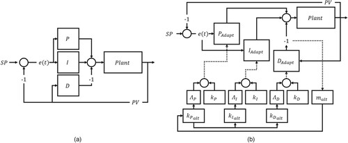
6.6. Controllers structures

Figure 4 shows a comparison between the $\mathrm{PID}$ parallel structure and the proposed $\mathrm{SeesawAPID}$ parallel structure.

Figure 4. Controllers: (a) $\mathrm{PID}$ with $D$ from $\mathrm{PV}$; (b) $\mathrm{SeesawAPID}$ with $D$ from $\mathrm{PV}$.

6.6.1. Parameters tuning

The gains of the $\mathrm{PID}$ controllers used as a base were tuned using the $\mathrm{PID}$ Tuner of Simulink®. Once these values were obtained, they remained unchanged for the adaptive controllers $\mathrm{API}{D}_{\mathrm{MS}}$ and $\mathrm{API}{D}_{\mathrm{LS}}$. The parameters for each algorithm were manually adjusted, following a Model-Based Tuning approach similar to heuristic $\mathrm{PID}$ tuning:

• $\mathrm{API}{D}_{\mathrm{MS}}$. Initial adjustment of $V_{\mathrm{om}}$ and $V_{\mathrm{oy}}$, followed by a progressive activation and adjustment sequence of ${\mathrm{\Lambda }}_P$, ${\mathrm{\Lambda }}_D$, and ${\mathrm{\Lambda }}_I$.

  • o $V_{\mathrm{om}}$ and $V_{\mathrm{oy}}$. Commencing with a 25/1 ratio, progressively decreasing it to 1/1.

• $\mathrm{API}{D}_{\mathrm{LS}}$. Initial adjustment of $V_{\mathrm{pct}}$, followed by a progressive activation and adjustment sequence of ${\mathrm{\Lambda }}_P$, ${\mathrm{\Lambda }}_D$, and ${\mathrm{\Lambda }}_I$.

  • o $V_{\mathrm{pct}}$. Commencing with a value of 0.99. It can be increased or decreased within the suggested range between 7 and 0.1.

Progressive activation and adjustment involve setting the limiter to 1 and gradually decreasing the value for enhanced control. The process is repeated for subsequent parameters. If optimal results aren't achieved, readjust the $\mathrm{APID}$ parameters and then the limiters again.

7. Simulation results

7.1. Algorithms demonstrations

In all demonstrations, the $e(t)$, $m_{\mathrm{orig}}$, and $m_{\mathrm{alt}}$ values of the corresponding algorithms were graphed, ($e(t)$ is represented as a sine wave). Consider $\mathrm{SP}=0$.

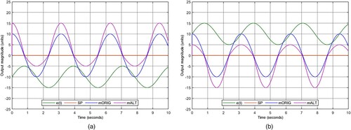
7.1.1. $m_{\mathrm{alt}}$ generation with MS seesaw algorithm

Figure 5 shows the $m_{\mathrm{alt}}$ values from Equations (10) and (13). It merely depicts the static calculation of the alternative slope ($m_{\mathrm{alt}}$) with the MS seesaw algorithm (for both converging and diverging signals) for positive and negative errors.

Figure 5. MS seesaw algorithm (a) when $-e(t)$, $V_{\mathrm{oy}}=1$, and $V_{\mathrm{om}}=2$. $m_{\mathrm{alt}}>m_{\mathrm{orig}}$ and (b) when $+e(t)$, $V_{\mathrm{oy}}=1$, and $V_{\mathrm{om}}=2$. $m_{\mathrm{alt}}<m_{\mathrm{orig}}$.

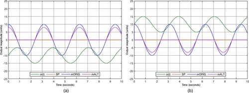
7.1.2. $m_{\mathrm{alt}}$ generation with LS seesaw algorithm

Figure 6 shows the $m_{\mathrm{alt}}$ values from Equation (21). It merely shows the calculation of $m_{\mathrm{alt}}$ with the LS seesaw algorithm for diverging signals when there are positive and negative errors.

Figure 6. LS seesaw algorithm (a) when $-e(t)$, $+m_{\mathrm{orig}}$, and $V_{\mathrm{pct}}=0.2$. $m_{\mathrm{alt}}<m_{\mathrm{orig}}$ and (b) when $+e(t)$, $-m_{\mathrm{orig}}$, and $V_{\mathrm{pct}}=0.2$. $m_{\mathrm{alt}}>m_{\mathrm{orig}}$.

7.2. Generic plant control with $\mathrm{API}{D}_{\mathrm{MS}}$ and $\mathrm{API}{D}_{\mathrm{LS}}$

A transfer function, $\mathrm{TF}$, is proposed: (43) $\mathrm{TF}=\frac{1}{(s+2)(s+3)(s+4)}=\frac{1}{s^3+9s^2+26s+24}$(43)

Table 1 shows the parameters for the $\mathrm{PID}$, the $\mathrm{API}{D}_{\mathrm{MS}}$, and the $\mathrm{API}{D}_{\mathrm{MS}}$ controllers.

Table 1. Controllers parameters.

	$\mathrm{PID}$	$\mathrm{API}{D}_{\mathrm{MS}}$	$\mathrm{API}{D}_{\mathrm{LS}}$
$k_P$	126	126	126
$k_I$	204.9	204.9	204.9
$k_D$	19.28	19.28	19.28
${\tau }_I$	0.153	0.153	0.153
${\tau }_D$	0.615	0.615	0.615
$V_{\mathrm{om}}$		25
$V_{\mathrm{oy}}$		1
$V_{\mathrm{pct}}$			7
${\mathrm{\Lambda }}_P$		0.65	0.075
${\mathrm{\Lambda }}_I$		0.0075	0.00095
${\mathrm{\Lambda }}_D$		1	0.25

$k_P$ is the proportional gain, $k_I$ is the integral gain, $k_D$ is the derivative gain, ${\tau }_I$ is the integral time,${\tau }_D$ is the derivative time, $V_{\mathrm{om}}$ is a variation over $m$, $V_{\mathrm{oy}}$ is a variation over $y$, $V_{\mathrm{pct}}$ is a percentage variation, ${\mathrm{\Lambda }}_P$ is the ${k_P}_{\mathrm{alt}}$ delimitation, ${\mathrm{\Lambda }}_I$ is the ${k_I}_{\mathrm{alt}}$ delimitation, and ${\mathrm{\Lambda }}_D$ is the ${k_D}_{\mathrm{alt}}$ delimitation.

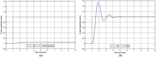
Figure 7 shows the responses to a step input (with a value of 1) of the open-loop and $\mathrm{PID}$-controlled system.

Figure 7. (a) Free response of the system; (b) $\mathrm{PID}$ controller response.

Figure 8 and Table 2 show the transient and stationary responses to a step input (with a value of 1) of the $\mathrm{PID}$ and the $\mathrm{SeesawAPID}$ controllers. Table 2 shows a quantitative comparison based on standard evaluation metrics obtained from the controller's signals (Abbas & Mustafa, 2023; Ogata, 2010).

Figure 8. (a) $\mathrm{PID}$ vs. $\mathrm{API}{D}_{\mathrm{MS}}$; (b) $\mathrm{PID}$ vs. $\mathrm{API}{D}_{\mathrm{LS}}$.

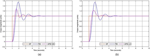
Table 2. Controllers comparison.

	$\mathrm{PID}$	$\mathrm{API}{D}_{\mathrm{MS}}$		$\mathrm{API}{D}_{\mathrm{LS}}$
$t_d$ (s)	1.375	1.243	−9.6%	1.238	−10.0%
$t_r$ (s)	1.545	1.397	−9.6%	1.433	−7.2%
$M_p$	1.544	1.287	−16.6%	1.222	−20.9%
$t_p$ (s)	1.901	1.614	−15.1%	1.715	−9.8%
$t_{s}2\text{\%}$ (s)	4.404	2.881	−34.6%	3.222	−26.8%
$t_{s}5\text{\%}$ (s)	3.650	2.750	−24.7%	2.161	−40.8%
$\mathrm{IAE}$	0.7801	0.3899	−50.0%	0.3723	−52.3%
$\mathrm{ISE}$	0.4265	0.2065	−51.6%	0.2015	−52.8%
$\mathrm{ITAE}$	1.4240	0.5926	−58.4%	0.5383	−62.2%
$\mathrm{ITSE}$	0.6098	0.2436	−60.1%	0.2366	−61.2%

$t_d$ is the delay time, $t_r$ is the rising time, $M_p$ is the maximum peak, $t_p$ is the peak time, $t_{s}2\text{\%}$ is the settling time at 2%, $t_{s}5\text{\%}$ is the settling time at 5%, $\mathrm{IAE}$ is the Integral Absolute Error, $\mathrm{ISE}$ is the Integral Squared Error, $\mathrm{ITAE}$ is the Integral Time Absolute Error, and $\mathrm{ITSE}$ is the Integral Time Squared Error.

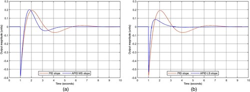
Figure 9 shows a slope comparison between the $\mathrm{PID}$ and the $\mathrm{SeesawAPID}$ controllers. The $\mathrm{API}{D}_{\mathrm{MS}}$ slope shows a more aggressive slope, and the $\mathrm{API}{D}_{\mathrm{LS}}$ slope shows a softened one, both correspond to its very nature.

Figure 9. (a) $\mathrm{PID}$ slope vs. $\mathrm{API}{D}_{\mathrm{MS}}$ slope; (b) $\mathrm{PID}$ slope vs. $\mathrm{API}{D}_{\mathrm{LS}}$ slope.

7.3. Equilibrium control of the IPC with $\mathrm{API}{D}_{\mathrm{MS}}$ and $\mathrm{API}{D}_{\mathrm{LS}}$

Table 3 shows the system parameters for the IPC.

Table 3. Parameters for the IPC.

Parameter	Value
$M$ (kg)	2.4
$m$ (kg)	0.23
$L$ (m)	0.36
$g$ (m/s^2)	9.81

$M$ is the cart’s mass, $m$ is the pendulum’s mass, $L$ is the pendulum’s length, and $g$ is gravity.

The parameters are substituted into Equations (40) and (41). (40) ${\dot{x}}_2=\frac{u+0.0828{x_4}^2\sin (x_3)-2.2563\cos (x_3)\sin (x_3)}{2.4+0.23{\sin }^2(x_3)}$(40) (41) ${\dot{x}}_4=\frac{\begin{array}{c}-\mathrm{ucos}(x_3)-0.0828{x_4}^2\sin (x_3)\cos (x_3)\\ +25.8003\sin (x_3)\end{array}}{0.864+0.0828{\sin }^2(x_3)}$(41)

Tables 4 and 5 show the parameters of the controllers.

Table 4. Equilibrium control parameters.

	$\mathrm{PID}$	$\mathrm{API}{D}_{\mathrm{MS}}$	$\mathrm{API}{D}_{\mathrm{LS}}$
$k_P$	−500
$k_I$	−750
$k_D$	−125
${\tau }_I$	0.25
${\tau }_D$	2/3
$V_{\mathrm{om}}$		1
$V_{\mathrm{oy}}$		1
$V_{\mathrm{pct}}$			0.1
${\mathrm{\Lambda }}_P$		0.001	0.95
${\mathrm{\Lambda }}_I$		0.01	0.5
${\mathrm{\Lambda }}_D$		0.05	0.1

Table 5. Position control parameters.

	$\mathrm{PID}$
$k_P$	−75
$k_I$	−25
$k_D$	−1
${\tau }_I$	75
${\tau }_D$	1/3

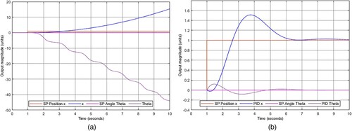
Figure 10 shows the responses of the free system and the equilibrium and position $\mathrm{PID}$-controlled system. Equilibrium's $\mathrm{SP}$ was set to 0°, a fully vertical standing, and the position's $\mathrm{SP}$ was set to 1.

Figure 10. (a) Free response of the system; (b) $\mathrm{PID}$ equilibrium control and $\mathrm{PID}$ position control responses.

Figure 11 compares the equilibrium control between the $\mathrm{PID}$ and $\mathrm{SeesawAPID}$ controllers. Table 6 shows an equilibrium control quantitative comparison using evaluation metrics for transient and stationary response stages (Abbas & Mustafa, 2023; Ogata, 2010).

Figure 11. Equilibrium control of (a) $\mathrm{PID}$ vs. $\mathrm{API}{D}_{\mathrm{MS}}$ and (b) $\mathrm{PID}$ vs. $\mathrm{API}{D}_{\mathrm{LS}}$.

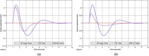
Table 6. Equilibrium control comparison.

	$\mathrm{PID}$	$\mathrm{API}{D}_{\mathrm{MS}}$		$\mathrm{API}{D}_{\mathrm{LS}}$
$t_d$ (s)
$t_r$ (s)	2.276	2.050	−9.9%	2.240	−1.6%
$M_p$	1.195e-1	1.034e-1	−13.5%	6.239e-2	−47.8%
$t_p$ (s)	1.466	1.384	−5.6%	1.300	−11.3%
$t_{s}2\text{\%}$ (s)	5.924	3.584	−39.5%	1.883	−68.2%
$t_{s}5\text{\%}$ (s)	3.958	2.906	−26.6%	1.519	−61.6%
$\mathrm{IAE}$	0.2522	0.1341	−46.8%	0.08436	−66.6%
$\mathrm{ISE}$	0.01721	0.00797	−53.7%	0.002463	−85.7%
$\mathrm{ITAE}$	0.7688	0.3	−61.0%	0.2301	−70.1%
$\mathrm{ITSE}$	0.04224	0.01506	−64.3%	0.004626	−89.0%

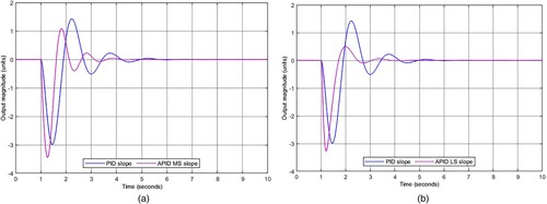
Figure 12 shows a slope comparison of the equilibrium control between the $\mathrm{PID}$ and $\mathrm{SeesawAPID}$ controllers. The $\mathrm{API}{D}_{\mathrm{MS}}$ generates a $m_{\mathrm{alt}}$ value greater than $m_{\mathrm{orig}}$ and The $\mathrm{API}{D}_{\mathrm{LS}}$ generates a $m_{\mathrm{alt}}$ value of less than $m_{\mathrm{orig}}$, which corresponds to its expected functionality.

Figure 12. (a) $\mathrm{PID}$ slope vs. $\mathrm{API}{D}_{\mathrm{MS}}$ slope; (b) $\mathrm{PID}$ slope vs. $\mathrm{API}{D}_{\mathrm{LS}}$ slope.

The use of algorithms for the equilibrium control affected the position control accordingly; Figure 13 graphs the corresponding affectation of each algorithm. Table 7 show the transient and stationary responses affected by the $\mathrm{SeesawAPID}$ controllers (Abbas & Mustafa, 2023; Ogata, 2010).

Figure 13. $\mathrm{PID}$ position control affected by (a) $\mathrm{API}{D}_{\mathrm{MS}}$ equilibrium control and by (b) $\mathrm{API}{D}_{\mathrm{LS}}$ equilibrium control.

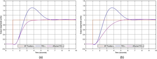
Table 7. Affected position control comparison.

	$\mathrm{PID}$	By $\mathrm{API}{D}_{\mathrm{MS}}$		By $\mathrm{API}{D}_{\mathrm{LS}}$
$t_d$ (s)	2.107	2.210	4.9%	2.676	27.0%
$t_r$ (s)	2.621	4.756	81.5%	5.332	103.4%
$M_p$	1.510	1.019	−32.5%	1.030	−31.8%
$t_p$ (s)	3.762	8.719	131.8%	7.311	94.3%
$t_{s}2\text{\%}$ (s)	6.278	3.771	−39.9%	20.854	232.2%
$t_{s}5\text{\%}$ (s)	5.927	3.380	−43.0%	4.610	−22.2%
$\mathrm{IAE}$	2.179	1.388	−36.3%	1.945	−10.7%
$\mathrm{ISE}$	1.304	0.9914	−24.0%	1.308	0.3%
$\mathrm{ITAE}$	6.435	2.963	−54.0%	4.848	−24.7%
$\mathrm{ITSE}$	2.908	1.556	−46.5%	2.382	−18.1%

8. Discussion

The seesaw algorithms focus on convergent signals towards an $\mathrm{SP}$, adapting to system changes but not necessarily controlling entirely different systems. They build upon a pre-existing $\mathrm{PID}$ to enhance its functionality.

The MS seesaw algorithm aims to achieve faster response than the original, accelerating signal approximation and facilitating quicker attainment of the $\mathrm{SP}$. However, it can lead to aggressive behaviour and oscillations rather than stabilization. It's advisable to deactivate it near the $\mathrm{SP}$ (6.3 Seesaw algorithms code for $\text{PID}$ control).

The LS seesaw algorithm aims to reduce signal perpendicularity, smoothing its approach to the $\mathrm{SP}$ and mitigating oscillations around it. The maximum $V_{\mathrm{pct}}$ value intended for the LS algorithm was 0.99 (99%). However, it was observed during development that this limit could be exceeded, resulting in significant improvements with values as high as 700%.

Throughout the development of the algorithms, ${\mathrm{\Lambda }}_I$ tended to destabilize the system, so minimal values were usually employed, resulting in similar outcomes between using $k_I$ or ${k_I}_{\mathrm{Adapt}}$. Despite these experiences, setting ${\mathrm{\Lambda }}_I$ to 0.5 significantly improved the IPC equilibrium control with the $\mathrm{API}{D}_{\mathrm{LS}}$ controller. Setting ${\mathrm{\Lambda }}_I$ at the minimum shouldn't be considered a steadfast rule.

For the tested systems, $\mathrm{SeesawAPID}$ controllers improved all signal rising and settling metrics and diminished maximum peak and error accumulation for both systems, fulfilling its goal and exhibiting its logic. For instance, the $\mathrm{API}{D}_{\mathrm{MS}}$ exhibits more oscillations and a longer settling time, $t_s$, but a shorter rising time, $t_r$, compared to the $\mathrm{API}{D}_{\mathrm{LS}}$. Conversely, the $\mathrm{API}{D}_{\mathrm{LS}}$ shows fewer oscillations and a shorter $t_s$, but a longer $t_r$, than the $\mathrm{API}{D}_{\mathrm{MS}}$.

Based on the $\mathrm{IAE}$, $\mathrm{ISE}$, $\mathrm{ITAE}$, and $\mathrm{ITSE}$ criteria used for evaluating controllers, the $\mathrm{API}{D}_{\mathrm{LS}}$ demonstrated superior performance for both plants. The seesaw algorithms enable the creation of faster and more accurate controllers compared to the $\mathrm{PID}$.

9. Future work

• The Seesaw algorithms can be applied within a convergent signal, enabling their use concurrently in a single instance.

• While it's understandable how changing the emerging parameters from the seesaw algorithms could affect outcomes, exploring tuning methods is essential.

• While it's clear how the seesaw algorithms’ emerging parameters can impact results, exploring tuning methods is crucial.

• The controllers can be systematically implemented by considering transfer functions from first to higher degrees.

• Addressing performance comparisons and combinations with other controllers is crucial. Given that these controllers are $\mathrm{PID}$-based, the range of options is extensive.

• The MS and LS algorithms provide two methods for proposing a slope. Exploring numerous other approaches could potentially yield better results.

Acknowledgements

The authors acknowledge CONAHCYT for providing a doctoral fellowship and CIDESI for the facilities, equipment, and software provided. Conceptualization, J.P.M.H. and J.C.S.V.; methodology, J.P.M.H.; software, J.P.M.H., C.H.S.S., and J.M.B.F; validation, J.P.M.H., D.M.O., and J.M.B.F.; investigation, J.P.M.H.; original draft preparation, J.P.M.H.; review and editing, J.P.M.H. and J.C.S.V.; supervision, J.C.S.V. All authors have read and agreed to the published version of this manuscript.

Disclosure statement

No potential conflict of interest was reported by the author(s).

References

- Abbas, I. A., & Mustafa, M. K. (2023). A review of adaptive tuning of PID-controller: Optimization techniques and applications. International Journal of Nonlinear Analysis and Applications, 15(2), 29–37. https://doi.org/10.22075/ijnaa.2023.21415.4024
- Ang, K. H., Chong, G., & Li, Y. (2005). PID control system analysis, design, and technology. IEEE Transactions on Control Systems Technology, 13(4), 559–576. https://doi.org/10.1109/TCST.2005.847331
- Åström, K. J., & Hägglund, T. (2001). The future of PID control. Control Engineering Practice, 9(11), 1163–1175. https://doi.org/10.1016/S0967-0661(01)00062-4
- Díaz-Rodríguez, I. D., Han, S., & Bhattacharyya, S. P. (2019). Analytical design of PID controllers. Springer International Publishing. https://doi.org/10.1007/978-3-030-18228-1
- Han, S.-Y., Dong, J.-F., Zhou, J., & Chen, Y.-H. (2022). Adaptive Fuzzy PID control strategy for vehicle active suspension based on road evaluation. Electronics, 11(6), 921. https://doi.org/10.3390/electronics11060921
- Johnson, M. A., Moradi, M. H., & Crowe, J. (2005). PID control: New identification and design methods; probability and its applications. Springer.
- Karanjkar, D. S., Chatterji, S., Kumar, A., & Shimi, S. L. (2014). Fuzzy adaptive proportional-integral-derivative controller with dynamic set-point adjustment for maximum power point tracking in solar photovoltaic system. Systems Science & Control Engineering, 2(1), 562–582. https://doi.org/10.1080/21642583.2014.956267
- Khan, L., Qamar, S., & Khan, U. (2016). Adaptive PID control scheme for full car suspension control. Journal of the Chinese Institute of Engineers, 39(2), 169–185. https://doi.org/10.1080/02533839.2015.1091427
- Mahmoodabadi, M. J., & Safi Jahanshahi, S. (2021). Optimal design of an adaptive robust proportional-integral-derivative controller based upon sliding surfaces for under-actuated dynamical systems. Cogent Engineering, 8(1), 1886738. https://doi.org/10.1080/23311916.2021.1886738
- Noordin, A., Mohd Basri, M. A., & Mohamed, Z. (2023). Real-time implementation of an adaptive PID controller for the quadrotor MAV embedded flight control system. Aerospace, 10(1), 59. https://doi.org/10.3390/aerospace10010059
- Ogata, K. (2010). Modern control engineering. Pearson.
- Prabhakar, G., Selvaperumal, S., & Nedumal Pugazhenthi, P. (2019). Fuzzy PD plus I control-based adaptive cruise control system in simulation and real-time environment. IETE Journal of Research, 65(1), 69–79. https://doi.org/10.1080/03772063.2017.1407269
- Prasad, L. B., Tyagi, B., & Gupta, H. O. (2011). Optimal control of nonlinear inverted pendulum dynamical system with disturbance input using PID controller & LQR. In 2011 IEEE International Conference on Control System, Computing and Engineering (pp 540–545). https://doi.org/10.1109/ICCSCE.2011.6190585.
- Prasad, L. B., Tyagi, B., & Gupta, H. O. (2012). Modelling and simulation for optimal control of nonlinear inverted pendulum dynamical system using PID controller and LQR. In 2012 Sixth Asia Modelling Symposium (pp. 138–143). https://doi.org/10.1109/AMS.2012.21.
- Prasad, L. B., Tyagi, B., & Gupta, H. O. (2014). Optimal control of nonlinear inverted pendulum system using PID controller and LQR: Performance analysis without and with disturbance input. International Journal of Automation and Computing, 11(6), 661–670. https://doi.org/10.1007/s11633-014-0818-1
- Swarnkar, P., Jain, S. K., & Nema, R. K. (2014). Adaptive control schemes for improving the control system dynamics: A review. IETE Technical Review, 31(1), 17–33. https://doi.org/10.1080/02564602.2014.890838
- Wang, W., Xu, L., & Hu, H. (2015). Neuron adaptive PID control for greenhouse environment. Journal of Industrial and Production Engineering, 32(5), 291–297. https://doi.org/10.1080/21681015.2015.1048752
- Wogi, L., Ayana, T., Morawiec, M., & Jąderko, A. (2022). A comparative study of fuzzy SMC with adaptive fuzzy PID for sensorless speed control of six-phase induction motor. Energies, 15(21), 8183. https://doi.org/10.3390/en15218183
- Zeng, S., Hu, H., Xu, L., & Li, G. (2012). Nonlinear adaptive PID control for greenhouse environment based on RBF network. Sensors, 12(5), 5328–5348. https://doi.org/10.3390/s120505328