An interpretable schizophrenia diagnosis framework using machine learning and explainable artificial intelligence

Abstract

Schizophrenia is a complicated and multidimensional mental condition marked by a wide range of emotional, cognitive, and behavioural symptoms. Although the exact root cause of schizophrenia is unknown, experts believe that a complex interaction of genetic, environmental, neurobiological, neurodevelopmental, and immune system dysfunctional elements are the contributing factors. In healthcare, artificial intelligence (AI) is used for analysing big datasets, enhance patient care, personalize treatment regimens, improve diagnostic accuracy, and expedite administrative duties. Hence, ML has been used to diagnose Schizophrenia in this study. The term ‘explainable artificial intelligence' (XAI) describes the development of AI systems that are able to provide understandable explanations for their choices as well as behaviours. In our research paper, we harnessed the power of five diverse XAI methodologies: LIME (Local Interpretable Model-agnostic Explanations), SHAP (Shapley Additive exPlanations), ELI5 (Explain Like I'm 5), QLattice, and Anchor. According to (XAI), the most significant attributes include age range, sex, the presence of a triradius on the left thumb, the total number of triradii, and the left thenar region's palmar pattern. By enabling early intervention, automatic identification of schizophrenia using XAI can benefit patients, assisting doctors in making precise diagnoses, assisting medical personnel in maximizing resource allocation and care coordination.

KEYWORDS:

• Artificial intelligence
• machine learning
• LIME
• schizophrenia
• SHAP

1. Introduction

A complex and disabling mental illness, schizophrenia affects around 1% of people on the planet marked by a serious disruption of mental and emotional functioning (Zhang, 2019). The perception of social relationships, cognitive abilities, intellectual processes, and reality are all impacted by this illness. Hallucinations (hearing voices or seeing things that are not there), mental disorders (atypical methods of thinking), and delusions (fixed, incorrect beliefs), are all signs of schizophrenia, as are decreased motivation to achieve goals, decreased emotional expression, motor impairments, difficulty forming and maintaining social connections and cognitive impairments (Oh et al., 2019; Siuly et al., 2020).

The nature and intensity of symptoms may vary over time, and there may be periods when they go worse before getting better. Certain symptoms might not go away. Men with schizophrenia typically experience symptoms in their early to mid-20s. Women typically begin to have symptoms in their late 20s. Diagnoses of schizophrenia are rare in children and far more common in adults over 45 (Schizophrenia - Symptoms and causes - Mayo Clinic, 2020). A doctor can determine whether a patient has schizophrenia or one of its related diseases by asking them questions, listening to them describe their symptoms, or watching them behave (Professional, C. C. M., n.d.a). The Diagnostic and Statistical Manual of Mental Disorder (DSM-5) (Professional, C. C. M., n.d.b) states that the following are necessary for a diagnosis of schizophrenia: A minimum of two of the five primary symptoms, for at least a month, one has experienced symptoms and the ability to work or maintain relationships – whether they be romantic, personal, or otherwise – is impacted by the symptoms (Professional, C. C. M., n.d.a). Schizophrenia can be treated, but doing so necessitates taking long-term drugs, which is extremely burdensome on families and healthcare systems (Siuly et al., 2022). Some of the treatment methods include: Antipsychotics, Other medications depending on the symptoms, Psychotherapy – therapies like cognitive behavioural therapy (CBT), Electroconvulsive therapy (ECT) etc, (Professional, C. C. M., n.d.a).

Schizophrenia, which is defined by its variability and the complexity of its underlying neurobiological mechanisms, poses a variety of difficulties for both patients and healthcare professionals. Machine learning (ML) which is a subset of AI is crucial because its complexity demands novel methodologies. To examine large and diverse datasets obtained from genetics, neuroimaging, and clinical assessments, ML technologies offer special capabilities. They can find intricate patterns, find new biomarkers, and disclose hidden links in the data by using advanced algorithms. Also, by enabling Early Intervention, Objective Assessment, Remote Monitoring, and Stigma Reduction for those living with this condition, automatic diagnosis of schizophrenia can have a number of positive effects on the mental healthcare industry.

Healthcare will be significantly changed by artificial intelligence (AI), machine learning (ML), and explainable AI (XAI). To aid in illness diagnosis, forecast patient outcomes, and improve treatment options, ML examine massive healthcare databases (Obermeyer & Emanuel, 2016). They improve diagnostic accuracy and timeliness by seeing minute patterns in patient records and images, which enables early diagnosis of diseases like cancer (Esteva et al., 2017). Predictive models powered by AI also assist healthcare personnel in making data-driven decisions, enhancing patient care and resource allocation (Caruana et al., 2015). Contrarily, XAI improves openness in AI-driven clinical choices by offering comprehensible justifications, boosting confidence, and promoting adoption among healthcare professionals (Carvalho et al., 2020). Together, these technologies support the delivery of healthcare that is more effective, precise, and individualized, which ultimately improves patient outcomes and lowers healthcare costs (Esteva et al., 2017; Obermeyer & Emanuel, 2016).

A few studies have used AI for schizophrenia diagnosis. Bae et al. (2021) used a machine learning method to identify schizophrenia from social media content. Utilizing the Push shift application programming interface, data was retrieved from Reddit (Pushshift., n.d.). To develop post data specifically for schizophrenia, public posts from the schizophrenia subreddit were gathered. The authors chose six non-mental health subreddits with an emphasis on living, exercise, and good feelings as a control group to make sure that the written posts were not specifically about schizophrenia (Low et al., 2020). Therefore, 16,462 users posted 60,009 original posts about schizophrenia and 248,934 individuals posted 425,341 original posts about the control group (Bae et al., 2021). Naive Bayes (NB), Random Forest (RF), Support Vector Machine (SVM), and Logistic Regression (LR), were used as ML classifiers, and Random Forest (RF) had the best accuracy of 96% for distinguishing between the control groups and schizophrenia. By utilizing machine learning, Parola et al. (2021) utilized Multimodal assessment of communicative-pragmatic aspects in schizophrenia. 32 schizophrenia patients and 35 healthy patients made up the data set. The Assessment Battery for Communication (ABaCo102), a validated test with high content validity, internal consistency, and inter-rater reliability was given to the participants (Bosco et al., 2012; Sacco et al., 2008). The decision tree algorithm was the focus of the authors’ effort, and the findings showed good overall performance with a mean Accuracy of 82%. Support vector machine learning was used by Ian, C.G. et al. (Gould et al., 2014) to classify multivariate neuroanatomical subgroups of cognitive symptoms in schizophrenia. 427 participants had access to structural MRI scans. 629 scans from the Australian Schizophrenia Research Bank (ASRB) are included in this subset. The authors categorized the grey  – and white-matter volume data from 134 healthy controls, 74 patients with cognitive deficit schizophrenia, and 126 patients with schizophrenia who had previously been classified as cognitive sparing subtype using support vector machine technology. This approach allowed for up to 72% accuracy in separating cognitive subtypes from healthy controls. S. Góngora Alonso et al.'s study (2022) compared various machine learning techniques for predicting individuals with schizophrenia who are admitted to hospitals. The eleven hospitals in the area's acute units were chosen by the authors. A total of 6933 people with various mental illnesses are included in the data collection, of whom 3002 have schizophrenia and 3931 have additional mental illnesses. Six algorithms, including k-NN, Random Forest, SVM, AdaBoost, Decision Tree, and Naive Bayes, were taken into consideration for the creation of the study. The study determines that the Random Forest ensemble algorithm, with accuracy 72.7%, is the most accurate at classifying hospitalized schizophrenia patients in this sample. Machine Learning Methods for the Event-Related Potential-Based Diagnosis of Schizophrenia by Santos Febles Elsa et al. (2022). 54 participants with schizophrenia and 54 healthy control people made up the study cohort. The purpose of this study was to compare the performance of the MKL classifier and the Boruta feature selection approach for single-subject classification of schizophrenia patients (SZ) and healthy controls (HC). After adopting Boruta feature selection, classification accuracy increased to 83% from 86% when utilizing the entire dataset.

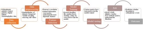
According to the few research described above, AI are being applied to many kinds of datasets in variety of ways to detect schizophrenia. We also emphasize Explainable AI (XAI) approaches like LIME, ELI5, QLattice, SHAP, and Anchor in this work. to learn more about how the algorithms choose their features and function. The findings cited above indicate that prediction has already been done using AI algorithms. The limits of schizophrenia include delayed diagnosis, lengthy psychiatric testing, non-corporative patients, etc. As mentioned earlier, schizophrenia is the most underlying psychiatric disease yet to be identified at the early stages for better assessment. Using the ML and XAI techniques, in a very short amount of time, assist the healthcare professionals in understanding the diagnosis, which can result in early detection, and what symptoms or features are the consequences of the diagnosis. The following ways that this article adds to an existing work of literature:

1. Pearson's correlation and mutual information feature selection approaches were used to identify the most crucial features.

2. Using baseline classifiers, a novel tailored ‘ensemble-stacking’ architecture was created and used to enhance performance.

3. To explain predictions, this original study used the five XAI algorithms LIME, SHAP, ELI5, QLattice, and Anchor on the given data.

The remainder of the manuscript is structured as follows: Materials and Methods are discussed in Section 2. The findings are discussed extensively in Section 3. Section 4 covers the classifiers’ conclusion and potential application.

2. Materials and methods

2.1 Dataset description

The Schizophrenia and Digital-Palmar Dermatoglyphics data in the Mendeley data were used to compile the dataset for this study (Arko-Boham, 2023). The dataset used in the study was cross-sectional and comprised the participation of 106 apparently healthy people in the community who had no family history of psychiatric disease as a control group and 69 patients with schizophrenia who had been diagnosed.

It has roughly 50 features (columns), of which 15 were categorical values and 35 were numerical. There are 69 people with a diagnosis of schizophrenia out of the 176 total participants,107 of them are not psychotic. There are 100 male patients on the participant list; 39 are in the control group and 61 are schizophrenic. Eight of the 76 female participants have schizophrenia, while the remaining 67 make up the control group. There are 37 participants between the ages of 18 and 20, 62 between the ages of 21 and 30, 22 between the ages of 31 and 40, 26 between the ages of 41 and 50, and 28 individuals over the age of 50.

The participants in the sample, who have different skin ridge morphologies on their palms and finger pads, comprise people with schizophrenia and those without schizophrenia or any other psychiatric diseases. It consists of research on the patterns and arrangements of the epidermal ridges on the palms and fingers, such as the triradius of the left thumb, the finger ridge count on the left index finger, and the triradius of the right thumb (Arko-Boham, 2023). Table 1 describes these features.

Table 1. Description of the features.

Sl. no	Feature name	Description	Sl. no	Feature name	Description	Sl. no	Feature name	Description
1	Participant	Control or Schizophrenia patient	18	Finger ridge count left index finger	No. of line present on the skin’s surface of the left index finger	35	Triradius right little finger	Three-ridge junction point on the right little finger
2	Sex	Gender of the participant	19	Triradius left index finger	Three-ridge junction point on the left index finger	36	Total finger ridge count left hand	Total no. of line present on the skin’s surfaces of all the finger in the left hand
3	Age range	Age range of the participants	20	Finger ridge count left middle finger	No. of line present on the skin’s surface of the left middle finger	37	Total finger ridge count right hand	Total no. of line present on the skin’s surfaces of all the finger in the right hand
4	Finger pattern left thumb	Finger pattern on the left thumb	21	Triradius left middle finger	Three-ridge junction point on the middle finger	38	Total finger ridge count	Total no. of lines present on the skin’s surfaces of all the fingers
5	Finger pattern left index finger	Finger pattern on the left index finger	22	Tinger ridge count left ring finger	No. of line present on the skin’s surface of the left ring finger	39	Total triradii left hand	Total three-ridge junction point in the left hand
6	Finger pattern left middle finger	Finger pattern on the left middle finger	23	Triradius left ring finger	Three-ridge junction point on the left ring finger	40	Total triradii right hand	Total three-ridge junction point in the right hand
7	Finger pattern left ring finger	Finger pattern on the left ring finger	24	Finger ridge count left little finger	No. of line present on the skin’s surface of the left little finger	41	Total triradii	Total three-ridge junction point on the palm or the finger
8	Finger pattern left little finger	Finger pattern on the left little finger	25	Triradius left little finger	Three-ridge junction point on the left little finger	42	a-b ridge count left hand	Count of ridges between two specific points a-b on the left hand
9	Finger pattern right thumb	Finger pattern on the right thumb	26	Finger ridge count right thumb	No. of line present on the skin’s surface of the right thumb	43	a-b ridge count right hand	Count of ridges between two specific points a-b on the right hand
10	Finger pattern right index finger	Finger pattern on the right index finger	27	Triradius right thumb	Three-ridge junction point on the right thumb	44	Total a-b ridge count	Total count of ridges between two specific points a-b
11	Finger pattern right middle finger	Finger pattern on the right middle finger	28	Finger ridge count right index finger	No. of line present on the skin’s surface of the right index finger	45	Palmar pattern left thenar region	Unique palm pattern near left thumb.
12	Finger pattern right ring finger	Finger pattern on the right ring finger	29	Triradius right index finger	Three-ridge junction point on the right index finger	46	Palmar pattern left hypothenar region	Unique palm pattern near base of left little finger
13	Finger pattern right little finger	Finger pattern on the right little finger	30	Finger ridge count right middle finger	No. of line present on the skin’s surface of the right middle finger	47	Palmar pattern right thenar region	Unique palm pattern near right thumb.
14	Palmar crease left hand	Palm lines on the left hand	31	Triradius right middle finger	Three-ridge junction point on the right middle finger	48	Palmar pattern right hypothenar region	Unique palm pattern near base of right little finger
15	Palmar crease right hand	Palm lines on the right hand	32	Finger ridge count right ring finger	No. of line present on the skin’s surface of the right ring finger	49	atd angle left hand/°	Angle measurement between the A (axial triradius), T (thenar triradius), and D (digital triradius) points on the palm of the left hand
16	Finger ridge count left thumb	No. of line present on the skin’s surface of the left thumb	33	Triradius right ring finger	Three-ridge junction point on the right ring finger	50	atd angle right hand/°	Angle measurement between the A (axial triradius), T (thenar triradius), and D (digital triradius) points on the palm of the right hand
17	Triradius of left thumb	Three-ridge junction point on the left thumb	34	Finger ridge count right little finger	No. of line present on the skin’s surface of the right little finger

2.2. Dataset preprocessing

Before using any machine learning technology, data preprocessing is an essential first step because the algorithms that learn from the data and the outcome of problem solving heavily depend on the relevant data, or features, that are needed to solve a particular problem. Preprocessing data entails a number of actions, such as eliminating null values, encoding of the categorical values to numerical values, normalization and data balancing techniques are some.

In this study 15 categorical and 35 numerical values are present. The categorical encoding is essential for machine learning methods since many machine learning algorithms, particularly those founded on mathematical equations, need on numerical input information. These algorithms cannot use categorical data, which represents categories or labels, as an input directly. To properly use machine learning models, categorical variables must be transformed into a numerical format using categorical encoding. The categorical values are manually encoded to the desired values. Encoding was done for all the 15 attributes.

To maintain computational performance (Zhang, 2018), prevent algorithmic bias (Bellamy et al., 2018), and assure data integrity, null values are deleted from datasets (Little & Rubin, 2019). In machine learning, handling missing data is crucial for accurate analysis and modelling. There was no null value attribute present in the dataset.

As a preprocessing method, normalization of a dataset ensures that feature values lie within a given range or have a mean of 0 and a standard deviation of 1. This procedure helps to avoid studies or machine learning models being dominated by features with distinct (James, Witten, et al., 2013). Depending on the data distribution and model needs, common techniques include (0, 1) scaling and z-score normalization (Peng et al., 2014). Normalization boosts interpretability and encourages more efficient model training. In the dataset used, all the features were normalized between 0 and 1.

Due to problems with class imbalance, data balancing is essential in machine learning. Biased models that underperform on minority classes can result from datasets that are unbalanced and have one class that considerably outnumbers the others. This bias has the potential to distort model performance measurements and model evaluation metrics (Japkowicz & Stephen, 2002). Different data balancing approaches, like as oversampling, under sampling, and the fabrication of synthetic data, are used to level the playing field and improve model accuracy and fairness to minimize this. All the classes in the selected dataset were balanced, and the predicted result data were also the same.

2.2.1. Feature selection

Feature selection is critical in machine learning for various reasons. First off, by lowering the chance of overfitting and ensuring that new data is well-generalized by the model, it is essential for improving model performance (Guyon & Elisseeff, 2003). Second, by making the dataset less dimensional, it improves computational efficiency by cutting down on the amount of time and resources needed for processing. Furthermore, feature selection encourages model interpretability, allowing stakeholders to develop understanding of the variables influencing model outcomes (Kohavi & John, 1997). By removing unimportant or noisy factors, It also contributes to improving the data's quality, leading to more precise forecasts. By concentrating on the most informative features, it also overcomes the dimensionality curse, a noteworthy issue with high-dimensional data analysis (Rand Corporation & Bellman, 1961). Pearson’s correlation and Mutual Information were the two techniques used in the research to extract the features.

2.2.1.1. Pearsons correlation

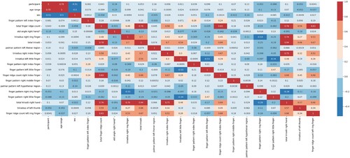
A statistical methodology used to evaluate the Pearson correlation is a linear relationship between two continuous variables. It assesses the strength and direction of the link from – 1 (completely negative correlation) to 1 (perfectly positive correlation), with 0 denoting no linear correlation. To find patterns and correlations in data, this coefficient is frequently employed in a variety of disciplines, including economics, the social sciences, and data analysis (Pearson, 1895). It is a crucial tool for machine learning feature selection and exploratory data analysis (Hastie et al., 2009). Figure 1 represents the persons correlation heatmap.

Figure 1. Heatmap of the Pearsons correlation.

2.2.1.2. Mutual Information

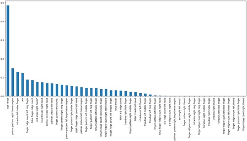
A statistical concept known as mutual information is used to express how dependent or information-sharing between two random variables is. With values ranging from 0 (no information shared) to higher values (more dependency), it calculates the amount of reduced ambiguity regarding one variable when the other is known (Cover, 1999). To find significant correlations between variables, this idea is frequently used in information theory, machine learning, and feature selection problems (Kraskov et al., 2004). Figure 2 represents the features by the mutual information algorithm.

Figure 2. The features are ranked in relevance by the Mutual Information Algorithm.

2.2.1.3. Important features

The key features from Table 2's Mutual information and Pearson's correlation are ‘age range’, ‘sex’, ‘palmar pattern left thenar region’, atd angle right hand/°, finger pattern right index finger, palmar pattern left hypothenar region, finger pattern right middle finger, finger pattern left index finger.

Table 2. Methods and the features.

Methods	Important features
Pearsons’s Correlation	‘age range’, ‘sex_14’, sex_13’, ‘palmar pattern left thenar region_12’, ‘a-b ridge count left hand’, ‘finger pattern left thumb _8’, ‘atd angle right hand/°’, finger pattern right index finger_5’, ‘finger pattern right thumb_2’, ‘finger pattern right index finger_6’, palmar pattern left thenar region_11’, ‘finger pattern left thumb _2’, ‘palmar pattern left hypothenar region_10’, ‘total a-b ridge count’, ‘palmar crease left hand’, ‘finger pattern right middle finger_6’, ‘palmar pattern right hypothenar region_11’, ‘palmar pattern right hypothenar region_10’, ‘finger pattern left index finger_8’, ‘finger pattern left index finger_6’.
Mutual Information	'participant’, ‘age range’,'sex’,'finger pattern left index finger’,'total finger ridge count’,'atd angle right hand/°’,'triradius right ring finger’,'total triradii’,'palmar pattern left thenar region’,'triradius right index finger’,'triradius left little finger’,'finger pattern right index finger’,'finger pattern left little finger’,'finger ridge count right index finger’,'finger pattern right middle finger’,'palmar pattern left hypothenar region’,'finger pattern right ring finger’,'finger pattern right little finger’,'total triradii right hand’,'triradius of left thumb’,'finger ridge count left ring finger’.

2.3. Machine learning methodology

Artificial intelligence is based on machine learning, which gives computers the capacity to pick up knowledge and impart it without explicit programming. This prominent topic includes a wide range of applications, from self-driving cars and improved medical diagnostics to systems that can recommend content and identify photographs. Algorithms and statistical models with deep roots in the field decipher complex data patterns by learning from examples and continuously improving performance. Unsupervised learning follows a route unrestricted by predefined data tags, whereas supervised learning trains models to make predictions using labelled data. In parallel, reinforcement learning equips entities to choose in dynamic, constantly changing situations. Machine learning has established itself as a vital and dynamic field, leading the forefront of technological development with its extensive impact on business and our everyday lives.

Numerous algorithms were employed to train the model. One of the most crucial elements in any ML that is utilized to influence the algorithm in our favour is the hyperparameters. It regulates the algorithms’ complexity and topology. Therefore, before fitting machine learning models to a data set, hyperparameters must be properly chosen (Jin, 2022). In machine learning, a hyperparameter is essentially anything whose values or configuration are chosen before training and whose choices will not change after training (Nyuytiymbiy, 2022). Grid-search is used to identify the optimal model hyperparameters, or those that yield the most ‘accurate’ predictions.

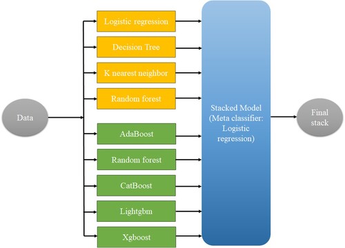
Machine learning models perform better when ensemble learning is used. Its underlying idea is straightforward. To create a more accurate model, various machine learning models are integrated (Kalirane, 2023). The three most prevalent ensemble learning approaches are stacking, boosting, and bagging. Each of these methods has a distinctive method for enhancing forecast accuracy (Kalirane, 2023). Three stacking techniques were used in our research. Stack 1 included classifiers such logistic regression, k-nearest neighbour, random forest, and decision tree. Tree-based methods like XgBoost, AdaBoost, Lightgbm, and CatBoost were included in the Stack 2. The two combined stacks made up the final stack. The customized stacking method is shown in Figure 3.

Figure 3. The Visual representation of customized stacking

Decision trees, naive bayes, logistic regression, random forests, k-Nearest Neighbours, and support vector machines are a few frequently used classifiers in machine learning (Hastie et al., 2009). The probabilities of binary outcomes are predicted by Logistic Regression, decision rules are created by Decision Trees based on input features, Random Forests employ collections of Decision Trees, Support Vector Machines look for the best data separation hyperplanes, k-Nearest Neighbours classify based on data proximity to neighbours, and Naive Bayes uses the Bayes theorem to estimate class probabilities (James, Witten, et al., 2013). These classification techniques are widely used in many machine learning fields, acting as reliable instruments for classification and prediction tasks (Han, Pei, et al., 2022).

Another model that is trained on a wide ensemble of models is called a voting classifier. It makes predictions about an output (class) depending on which of the selected classes has the highest probability of occurring. In our investigation, we used two voting methods: hard voting and soft voting. SVM, Logistic regression and decision tree were ensembled to get the best outcome. The Voting method is depicted in Figure 4. The steps followed in the study are given in the Figure 5.

Figure 4. Represents the Flow chat of the voting methodology used in the study.

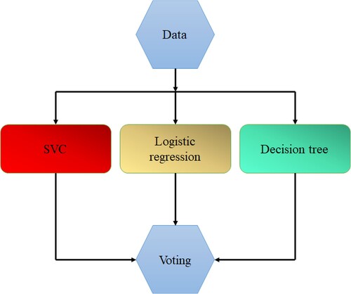
Figure 5. The pipeline of the machine learning methodology used in the study.

XAI techniques were applied to interpret the model outputs. The XAI techniques applied in this research were:

• SHAP (SHapley Additive exPlanations)  – Utilizes Shapley values from game theory to explain model outputs by allocating credit optimally (Dallanoce & Explainable, 2022).

• LIME (Local Interpretable Model-agnostic Explanations)  – meant to provide accessible insights into complicated machine learning model predictions by mimicking their behaviour in limited parts of the data space, making it easier to grasp how the model arrives at specific judgments (Amarasinghe et al., 2023)

• ELI5 (Explain Like I'm 5)  – method that simplifies difficult machine learning model explanations to make them easily intelligible, like describing things to a 5-year-old.

• QLattice  – Qlattice is a XAI method that uncovers patterns and explains the behaviour of complicated machine learning models using a novel methodology influenced by quantum physics.

• Anchor  – The idea of anchors, which are highly precise principles, is to explain how complex models behave (Dallanoce & Explainable, 2022).

2.4. Deep learning methodology

These days, deep learning (DL), a subfield of artificial intelligence (AI) and machine learning (ML), is regarded as a fundamental technology. Owing to its capacity for data-driven learning, deep learning (DL) technology – which has its roots in artificial neural networks (ANNs) – has gained significant traction in the computer community and finds widespread use across a wide range of industries, including cybersecurity, healthcare, visual identification, and text analytics (Khare et al., 2023). However, because real-world problems and data are dynamic and vary, developing a suitable deep learning model is a difficult undertaking. Furthermore, the absence of fundamental knowledge renders deep learning techniques opaque, impeding standard development (Sarker, 2021). There are 3 deep learning models which are trained for the dataset and those are 1D-CNNs have been proposed and immediately achieved the state-of-the-art performance levels in several applications such as personalized biomedical data classification and early diagnosis, structural health monitoring, anomaly detection (Han, Nianyin, et al., 2022; Serkan et al., 2021), Artificial neural network (ANN) which is used to replicate the nodes in the human brain and Long short-term memory (LSTM) network is a recurrent neural network (RNN), aimed to deal with the vanishing gradient problem present in traditional RNNs (Sepp & Jürgen, 1997).

3. Results

3.1. Performance metrics

The degree to which a measurement is accurate depends on how closely it resembles the object's real dimensions is termed as accuracy. (1) $\begin{array}{rl}\mathbf{\text{Accuracy}}& =(\mathbf{\text{True}}\mathbf{\text{Positives}}+\mathbf{\text{True}}\mathbf{\text{Negatives}})/\\ & (\mathbf{\text{True}}\mathbf{\text{Positives}}+\mathbf{\text{True}}\mathbf{\text{Negatives}}\\ & +\mathbf{\text{False}}\mathbf{\text{Positives}}+\mathbf{\text{False}}\mathbf{\text{Negatives}})\end{array}$(1) The proportion of real positive predicts among all positive predictions is referred to as precision. (2) $\begin{array}{rl}\mathbf{\text{Precision}}& =\mathbf{\text{True}}\mathbf{\text{Positives}}/\\ & (\mathbf{\text{True}}\mathbf{\text{Positives}}+\mathbf{\text{False}}\mathbf{\text{Positives}})\end{array}$(2)

The fraction of true positives among all actual positives is measured by recall, which is referred to as sensitivity. (3) $\begin{array}{rl}\mathbf{\text{Recall}}& =\mathbf{\text{True}}\mathbf{\text{Positives}}/\\ & (\mathbf{\text{True}}\mathbf{\text{Positives}}+\mathbf{\text{False}}\mathbf{\text{Negatives}})\end{array}$(3) The F1 score is calculated as the harmonic average of precision and recall. (4) $\begin{array}{rl}\mathbf{\text{F1}}\mathbf{\text{score}}& =\mathbf{\text{2}}\ast (\mathbf{\text{Precision}}\ast \mathbf{\text{Recall}})/\\ & (\mathbf{\text{Precision}}+\mathbf{\text{Recall}})\end{array}$(4)

The AUC (Area Under the ROC Curve) evaluates the model's capacity to differentiate between classes by measuring the area under the Receiver Operating Characteristic curve, which typically ranges from 0 to 1.

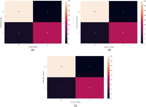
A table that summarizes the model's predictions by contrasting them with the actual values is called a confusion matrix. Comprising of True Negatives, False Negatives, True Positives and False Positives.

3.2. Model evaluation

Using machine learning algorithms, we were able to determine if the patient was schizophrenic or not, as well as which features led to the identification of the same. This will assist medical practitioners, particularly those in the mental healthcare industry, in the early diagnosis of disease and in the identification of disease faster than traditional analysis. The classifiers were tested in the Conda virtual environment, which is integrated with Python. Scikit, NumPy, Pandas, seaborn, and matplotlib were among the libraries installed. The models were trained on an ‘Intel® core (TM) i5’ CPU with 16 GB of RAM. For this investigation, a 64-bit version of the Windows operating system was used.

All the models were trained using an 80:20 ratio of training to testing. We have used five-fold cross validation technique. Table 3 summarizes the findings of multiple ML models for Pearson's correlation and Mutual information. All the data were balanced, and three models provided the best algorithms: Logistic Regression, with, precision, F1, accuracy, and recall scores of 0.85, 0.84, 0.86, 0.84, SVM  – linear kernel, with accuracy, recall, precision, and F1 scores of 0.86, 0.84, 0.85, 0.84 and Ridge, with accuracy, precision, recall, and F1 scores of 0.86, 0.85, 0.84, 0.84.

Table 3. All the classifiers with its accuracy, precision, recall and F1 score.

Models	Accuracy	Precision	Recall	F1 – score
Random forest	0.83	0.83	0.80	0.81
Logistic Regression	0.86	0.85	0.84	0.84
Decision Tree	0.83	0.83	0.80	0.81
KNN	0.66	0.62	0.59	0.58
SVM – linear kernel	0.86	0.85	0.84	0.84
SVM – sigmoid kernel	0.51	0.38	0.42	0.39
Stack 1	0.83	0.82	0.82	0.82
AdaBoost	0.83	0.82	0.82	0.82
CatBoost	0.83	0.82	0.82	0.82
LGBM	0.83	0.82	0.82	0.82
XGB	0.80	0.79	0.78	0.78
Stack 2	0.80	0.79	0.78	0.78
Final Stack	0.80	0.79	0.78	0.78
Hard voting	0.85	0.87	0.82	0.84
Soft voting	0.80	0.80	0.76	0.77
C4.5 (Decision Tree)	0.82	0.83	0.80	0.81
CART	0.82	0.82	0.82	0.82
Ridge	0.86	0.85	0.84	0.84

Figures 6 show the AUC curves for Logistic regression, SVM  – linear kernel, and Ridge classifiers. When Pearson's correlation and Mutual information were used, the AUC were 93%, 91%, and 94%, respectively. Figure 7 illustrate the precision-recall (PR) curves for the Logistic regression, SVM  – linear kernel, and Ridge classifiers. Pearson's correlation and mutual information techniques achieved precisions of 88%, 87%, and 90%, respectively. Figures 8 show the confusion matrix of the Logistic regression, SVM  – linear kernel, and Ridge classifiers. This study integrated heterogeneous classifiers with feature selection techniques to improve these classifiers’ performance. Hospitals can utilize these models to assist physicians in diagnosing schizophrenia.

Figure 6. AUC curves for (a) Logistic regression, (b) SVM – linear kernel, (c) Ridge classifier

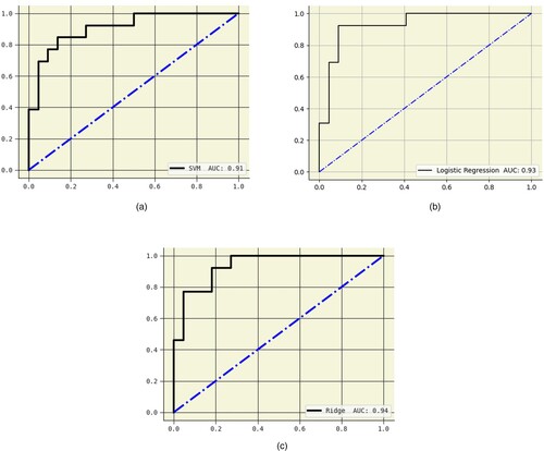
Figure 7. Precision-recall (PR) (a) Logistic regression, (b) SVM – Linear kernel, (c) Ridge classifier

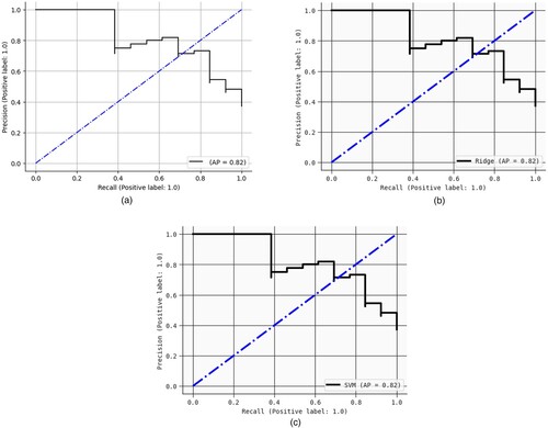
Figure 8. Confusion matrix of (a) Logistic regression, (b) SVM – linear kernel, (c) Ridge Classifier

3.3. Explainable artificial intelligence (XAI)

The methods by which DL and ML models’ study and form predictions are unknown to their developers (Amarasinghe et al., 2023; Arrieta et al., 2020; Langer et al., 2021; NetApp., 2019). As a result, decision-makers, or end user, inherently run the danger of placing their reliance in a system that is unable to articulate itself when making crucial judgments (Adadi & Berrada, 2018). Considering this, Explainable AI (XAI) was developed to assist users in comprehending how particular outputs from an AI-enabled system are produced.

This study has employed five XAI techniques: Eli5, Anchor, SHAP, QLattice, and LIME. By applying the feature importance approaches previously mentioned, we can gain a clearer understanding of the significance of attributes. Here we used the best 20 attributes for the interpretation.

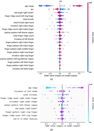
SHAP (SHapley Additive exPlanations) is an interpretable machine learning framework that aims to explain any output produced by a machine learning model. Its foundation is the idea of Shapley values, which come from the theory of cooperative games (Lundberg & Lee, 2017). Shapley values, which show how each feature contributes to the final prediction, offer a means of equitably dividing the ‘value’ of a prediction among the input features. The main concept is to consider every conceivable combination of features and track how the forecast changes when certain features are added or removed. After that, these values are combined to provide a fair and understandable feature importance metric (Lundberg et al., 2018). The beeswarm plot generated by the SHAP study for local interpretation is displayed in Figure 9. Based on the image (a), we can deduce that the patient's age range and sex are the primary characteristic that helps determine whether or not the patient has schizophrenia. The image (b) accepts any model and masker combination and yields a callable subclass object that carries out the selected estimating procedure and we can understand that age range is the important feature.

Figure 9. Beeswarm plot for SHAP (a) Beeswarm plot of 20 features (b) SHAP explainers for the 20 features

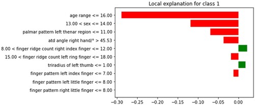
An XAI technique called LIME (Local Interpretable Model-agnostic Explanations) explains each prediction that intricate machine learning models make (Lundberg et al., 2018; Lundberg & Lee, 2017; Ribeiro et al., 2016a; Ribeiro et al., 2016b; Smith & Rajendra, 2023). It starts with a chosen instance, produces perturbed data, and creates a local approximation of the black-box model using a stand-in interpretable model. This surrogate model provides the feature importance needed to justify the forecast (Chadaga, Prabhu, et al., 2023; Miller, 2019). In our study the LIME explains that the red colour like age range, sex and palmer pattern left thenar region showed to be the prominent attributes for schizophrenia and the green colour represents the attributes for the control which is represented in Figure 10.

Figure 10. Attributes contributing for schizophrenic and not are represented by LIME.

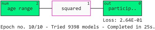
The QLattice simulation makes use of quantum-inspired decision-making to help us understand the interactions seen in the data. The results are interpreted using QGraphs. These graphs are made up of registers, edges and activation functions. Every attribute is given a register, and edges are used connect them. The registers are then subjected to activation processes to produce insightful data (Caruana et al., 2015). Figure 11 shows the QGraph of the study. It is evident that the age range is the most crucial factor in the schizophrenia prediction. The ‘squared’ function is also used to understand the outcomes.

Figure 11. Model predictions explained with QGraph.

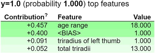
An XAI technique called ELI5 (Explain Like I'm 5) breaks down intricate machine learning models into clear-cut justifications (Guidotti et al., 2018). It simplifies model predictions so that even non-experts may understand them through the use of simple language and graphics. Important aspects are usually highlighted by ELI5, along with how they affect predictions (Islam et al., 2022; Korobov & Lopuhin, 2016). A Python module called Eli5 (Rahimi et al., 2023) explains machine learning models, thereby converting them from ‘black box’ to ‘white box’ versions. It works with multiple machine learning libraries, such as XGBoost models, Keras, and the Scikit-Learn library. The Eli5 method and Random Forest feature weight evaluation is quite similar. The ensemble of trees’ decision splits is followed to determine the weights. The contribution score is based on how much each node's output score varies from parent to child node. The ‘bias’ score and the total feature contributions are used to make the forecast. Figure 12 shows the important features i.e. age range, triradius of left thumb and total triradii that are contributing by the ELI5 explanation technique (Chadaga, Sampathila, et al., 2023).

Figure 12. Eli5 to explain model predictions.

To demystify the models, anchors provide explanations based on rules (Parsa et al., 2020). Users comprehend the forecasts under a set of conditions. The anchor explanations for patients with and without schizophrenia are displayed in Table 4. Evaluation measures are utilized to verify each anchor, including coverage and precision (Mokhtari et al., 2019).

Table 4. Five patients with schizophrenia and five patients without schizophrenia had anchor explanations.

Instance	Patient prediction	Anchor condition	Precision	Coverage
1	Control	age range < =  16.00 AND atd angle right hand/° > 42.62	1.00	0.34
2	Control	age range > 16.00 AND total triradii > 10.00	0.90	0.30
3	Control	age range < =  16.00 AND finger pattern right ring finger < =  7.00	1.00	0.21
4	Control	age range < =  16.00 AND finger ridge count left ring finger > 15.00	1.00	0.28
5	Control	age range < =  16.00 AND atd angle right hand/° > 42.62	0.99	0.35
6	Schizophrenic	age range > 16.00 AND triradius of left thumb < =  1.00	0.89	0.29
7	Schizophrenic	age range > 16.00 AND finger ridge count right index finger > 15.00	0.87	0.10
8	Schizophrenic	age range > 16.00 AND total triradii > 10.00	0.90	0.29
9	Schizophrenic	age range > 18.00 AND triradius of left thumb < =  1.00	0.96	0.11
10	Schizophrenic	age range > 18.00 AND atd angle right hand/° > 45.53	0.95	0.03

The XAI methodologies discussed above show that the beeswarm plot demonstrates how all the variables work together to predict schizophrenia in relation to SHAP. The force plot only shows the most important characteristics that enhance schizophrenia prediction (Kumarakulasinghe et al., 2020; Zafar & Khan, 2021). SHAP can be interpreted locally as well as globally. When comparing the feature importance to other XAI methodologies, a variety of visualization charts are provided. The contribution of each attribute to the schizophrenia prediction can be seen in LIME. For those who have survived – that is, who did not suffer from schizophrenia – we have created visualizations (Riyantoko & Diyasa, 2021; Shwartz-Ziv & Armon, 2022). We discover the attribute weights in LIME. However, the understanding we have here is local in nature rather than global. This implies that with LIME, greater in-depth analysis is only possible for individual patient forecasts. Qlattice provides a transfer equation to back up the assertion and illustrates which critical characteristics cause schizophrenia (Kawakura et al., 2022; Negara et al., 2021). Qlattice trains the model to recognize predictions by utilizing the popular quantum computing approach. But when compared to other approaches, it requires a lot of processing effort and resources. The relative significance of each characteristic in predicting schizophrenia is shown by Eli5 (Ribeiro et al., 2018). Eli5 is an incredibly effective method for tree-based models, including random forests and decision trees. However, as of right now, deep learning classifiers and other baseline models, such as Eli5, are not supported. Lastly, he uses logical justifications to show how exactly the traits might predict schizophrenia (Arias & Astudillo, 2023; Gallagher et al., 2017). While we can achieve the visualization graphs without the use of an anchor, we may use it to determine the optimal markers based on certain parameters. Plots for visualization are accessible with all other approaches, with the exception of anchor.

3.4. Deep learning (DL)

In this work, three deep learning models are employed. An 80:20 training-to-testing ratio was used for each model. With an accuracy of 83%, the 1D-CNN produced the best results out of all the DL models. The DL models demonstrated good performance in the diagnosis of schizophrenia. The models would have performed better if the data set was more as the results were overfitting (Dataset OSF, 2020).

4. Discussion

In this study, machine learning was used to forecast the likelihood that a patient may have schizophrenia. 175 patients in all (69 schizophrenia and 106 control) were taken into consideration. The feature selection technique made use of Pearson's correlation and mutual information. A variety of machine learning models were employed, including Random Forest, Decision Tree, Logistic Regression, SVM  – linear kernel, KNN, SVM  – sigmoid kernel, Stack 1 (LR, DT, KNN), LGBM, AdaBoost, XGB, CatBoost, Stack 2 (AdaBoost, RF, LGBM, CatBoost, XGB), Hard voting, Soft voting, Final stack (Stack 1, Stack 2), C4.5, CART, and Ridge classifiers. Five XAI techniques (LIME, ELI5, Anchor, QLattice, and SHAP) were applied in order to decipher the ML models’ ‘black box’. As a key decision support system, the ML models assist in the detection of schizophrenia.

We may infer from the XAI models that a person's age range is a significant factor in deciding whether or not they are schizophrenia. Most cases of schizophrenia are seen in those between the ages of 41 and 50. The other characteristics, such as total triradii, the triradius of the left thumb, and the atd angle of the right hand/°, also explain the major risk factors for schizophrenia. Our research also indicates that male patients are more likely than female patients to be diagnosed with schizophrenia.

Numerous machine learning approaches have been used in several research to improve schizophrenia prediction. Arias and Astudillo (2023) used a variety of machine learning methods to forecast patients’ risk of schizophrenia by analysing electroencephalogram (EEG) data using ML algorithms and the SHAP XAI technique. The data set ‘Identifying Psychiatric Disorders Using Machine-Learning (Dataset)’ (Arias & Astudillo, 2023) is used in this investigation. Extreme Gradient Boosting (XGBoost), Support Vector Machines (SVM), and Adaptive Boosting (AdaBoost), are the three classifiers that are compared. The classification process is measured using three metrics: F-l score (F1), area under the curve (AUC), and accuracy (ACC). The pipeline incorporates XAI to find pertinent features. With an ACC = 0.93, The model that does the best at predicting occurrences of schizophrenia is called XGBoost. Applying the SHAP explainability technique to the XGBoost model revealed that the most significant features in the prediction processes were the IQ, sex, delta Pz, and delta T6 waves. Hofmann et al. (2022) used an appropriate machine learning approach to investigate inpatient aggressiveness in offender patients with schizophrenia spectrum disorders (SSDs). There were 370 patients in the dataset. Support vector machines (SVM), with a balanced accuracy of 77.6%, beat all other machine learning techniques. According to a study by Góngora Alonso, et al. (2023), the purpose of this paper is to use machine learning algorithms to predict the readmission risk of patients with schizophrenia in an area of Spain. dataset comprising 3065 patients with schizophrenia illnesses and 6089 electronic admission records. Eleven public hospitals’ acute units in a particular region of Spain provided the data between 2005 and 2015. In terms of readmission risk prediction, the Random Forest classifier performed the best, with an accuracy of 0.817 (Zhu et al., 2021). Using retinal fundus pictures, a trained convolution neural network (CNN) deep learning algorithm was used in a recent study by Abhishek et al. to detect SCZ. Using a fundus camera, retinal pictures of 327 subjects – 139 patients diagnosed with schizophrenia (SCZ) and 188 healthy volunteers (HV) – were gathered. With an AUC of 0.98, the CNN classified SCZ and HV with 95% accuracy (Aslan & Akin, 2022). Table 5 compares our suggested methodology with the models that are currently in use.

Table 5. Comparison between our proposed model and the existing models.

Sl.no	Model	Classifiers	Accuracy	Explainable AI Techniques
1	(Riyantoko & Diyasa, 2021)	SVM, XGBoost and AdaBoost	93%	SHAP
2	(Kawakura et al., 2022)	Trees, Logistic regression, Random forest, KNN, Gradient boosting, Naive Bayes and SVM	77.6%	No
3	(Gallagher et al., 2017)	Random forest, Logistic regression, MPL, AdaBoost, SVM radial, XGBoost	81.7%	No
4	Our proposed model	Random forests, Decision trees, Logistic regression, KNN, SVM (Linear, sigmoidal), AdaBoost, LGBM, CatBoost, XGBoost, Hard and soft voting, C4.5, CART, Ridge and stacking models	86%	SHAP, LIME, QLattice, Anchor, ELI5

Our model provides an excellent summary of the models that we have modified to predict the occurrence of schizophrenia in patients; nevertheless, before implementing this framework in any healthcare setting, a thorough investigation into testing, external verification, and scalability evaluations should be carried out. If a larger dataset is being considered, additional deep learning can be used to enhance model understanding. Holdout validation can also be carried out.To bridge the expertise gap between medical professionals and informatics, the model should be just as useful to medical professionals as it is to a machine learning specialist. This proposed application is linked to SDG-3.

5. Conclusion

One mental health issue that needs to be identified early in order to receive treatment and lower the chance of problems is schizophrenia. Our proposed study included 175 participants with 50 attributes in total. Using mutual information and Pearson’s correlation coefficient, the most crucial characteristics from the 50 were identified. Ridge classifier, SVM (linear), and logistic regression all achieved maximum accuracy of 86%. The five XAI approaches that were applied were Anchor, SHAP, LIME, QLattice, and ELI5. The three most crucial characteristics for diagnosing schizophrenia were found to be age range, sex, and total triradii. The suggested approach was also evaluated against other relevant studies to determine how well it established classifier reliability. Medical professionals can utilize the classifiers as a decision support system to anticipate schizophrenia. This system could be expanded to foresee schizophrenia in a larger population if real-time prediction is put into practice.

Credit author statement

Samhita Shivaprasad: Software, Writing – Original draft preparation. Krishnaraj Chadaga: Conceptualization, Methodology. Cifha Crecil Dias: Visualization, Investigation. Niranjana Sampathila: Supervision. Srikanth Prabhu: Reviewing and Editing.

Disclosure statement

No potential conflict of interest was reported by the author(s).

Data availability statement

Data will be made available after obtaining prior permission from the corresponding author.

References

- Adadi, A., & Berrada, M. (2018). Peeking inside the black-box: A survey on explainable artificial intelligence (XAI). IEEE Access, 6, 52138–52160.
- Amarasinghe, K., Rodolfa, K. T., Lamba, H., & Ghani, R. (2023). Explainable machine learning for public policy: Use cases, gaps, and research directions. Data & Policy, 5, e5.
- Arias, J. T., & Astudillo, C. A. (2023). Enhancing Schizophrenia Prediction Using Class Balancing and SHAP Explainability Techniques on EEG Data. In 2023 IEEE 13th International Conference on Pattern Recognition Systems (ICPRS) (pp. 1-5). IEEE.
- Arko-Boham, B. (2023). Schizophrenia and Digital-Palmar dermatoglyphics. Mendeley Data. https://doi.org/10.17632/p2hds3wj2h.6
- Arrieta, A. B., Díaz-Rodríguez, N., Del Ser, J., Bennetot, A., Tabik, S., Barbado, A., … Herrera, F. (2020). Explainable artificial intelligence (XAI): Concepts, taxonomies, opportunities and challenges toward responsible AI. Information Fusion, 58, 82–115.
- Aslan, Z., & Akin, M. (2022). A deep learning approach in automated detection of schizophrenia using scalogram images of EEG signals. Physical and Engineering Sciences in Medicine, 45(1), 83–96.
- Bae, Y. J., Shim, M., & Lee, W. H. (2021). Schizophrenia detection using machine learning approach from social media content. Sensors, 21(17), 5924. https://doi.org/10.3390/s21175924
- Bellamy, R. K., Dey, K., Hind, M., Hoffman, S. C., Houde, S., Kannan, K., … Zhang, Y. (2018). AI Fairness 360: An extensible toolkit for detecting, understanding, and mitigating unwanted algorithmic bias. arXiv preprint arXiv:1810.01943.
- Bosco, F. M., Angeleri, R., Zuffranieri, M., Bara, B. G., & Sacco, K. (2012). Assessment battery for communication: Development of two equivalent forms. Journal of Communication Disorders, 45(4), 290–303.
- Caruana, R., Lou, Y., Gehrke, J., Koch, P., Sturm, M., & Elhadad, N. (2015). Intelligible models for healthcare: Predicting pneumonia risk and hospital 30-day readmission. In Proceedings of the 21th ACM SIGKDD international conference on knowledge discovery and data mining (pp. 1721-1730).
- Carvalho, D., Novais, P., Rodrigues, P., Machado, J., & Neves, J. (2020). Explainable artificial intelligence model for early diagnosis of COVID-19 using X-ray images. Information Fusion, 68, 146–157.
- Chadaga, K., Prabhu, S., Bhat, V., Sampathila, N., Umakanth, S., & Chadaga, R. (2023). A decision support system for diagnosis of COVID-19 from Non-COVID-19 influenza-like illness using explainable artificial intelligence. Bioengineering, 10(4), 439.
- Chadaga, K., Sampathila, N., Prabhu, S., & Chadaga, R. (2023). Multiple explainable approaches to predict the risk of stroke using artificial intelligence. Information, 14(8), 435.
- Cover, T. M. (1999). Elements of information theory. John Wiley & Sons.
- Dallanoce, F., & Explainable, A. I. 2022. A Comprehensive Review of the Main Methods, MLearning.ai, January 5, 2022.
- Dataset OSF. 2020. The dataset used in this study is publicly available and can be accessed at the following URL: https://osf.io/8bsvr/
- Esteva, A., Kuprel, B., Novoa, R. A., Ko, J., Swetter, S. M., Blau, H. M., & Thrun, S. (2017). Dermatologist-level classification of skin cancer with deep neural networks. nature, 542(7639), 115–118.
- Gallagher, R. J., Reing, K., Kale, D., & Ver Steeg, G. (2017). Anchored correlation explanation: Topic modeling with minimal domain knowledge. Transactions of the Association for Computational Linguistics, 5, 529–542.
- Góngora Alonso, S., Herrera Montano, I., Ayala, J. L. M., Rodrigues, J. J., Franco-Martín, M., & de la Torre Díez, I. (2023). Machine learning models to predict readmission risk of patients with Schizophrenia in a Spanish Region. International Journal of Mental Health and Addiction, 1–20.
- Góngora Alonso, S., Marques, G., Agarwal, D., De la Torre Díez, I., & Franco-Martín, M. (2022). Comparison of machine learning algorithms in the prediction of hospitalized patients with schizophrenia. Sensors, 22(7), 2517.
- Gould, I. C., Shepherd, A. M., Laurens, K. R., Cairns, M. J., Carr, V. J., & Green, M. J. (2014). Multivariate neuroanatomical classification of cognitive subtypes in schizophrenia: A support vector machine learning approach. NeuroImage: Clinical, 6, 229–236.
- Guidotti, R., Monreale, A., Ruggieri, S., Turini, F., Giannotti, F., & Pedreschi, D. (2018). A survey of methods for explaining black box models. ACM computing surveys (CSUR, 51(5), 1–42.
- Guyon, I., & Elisseeff, A. (2003). An introduction to variable and feature selection. Journal of Machine Learning Research, 3(Mar), 1157–1182.
- Han, L., Nianyin, Z., Peishu, W., & Kathy, C. (2022). Cov-Net: A computer-aided diagnosis method for recognizing COVID-19 from chest X-ray images via machine vision. Expert Syst. Appl, 207, 1–12. https://doi.org/10.1016/j.eswa.2022.118029
- Han, J., Pei, J., & Tong, H. (2022). Data mining: Concepts and techniques (4th ed.). Morgan kaufmann.
- Hastie, T., Tibshirani, R., Friedman, J. H., & Friedman, J. H. (2009). The elements of statistical learning: Data mining, inference, and prediction (Vol. 2, pp. 1-758). springer.
- Hofmann, L. A., Lau, S., & Kirchebner, J. (2022). Advantages of machine learning in forensic psychiatric research—uncovering the complexities of aggressive behavior in schizophrenia. Applied Sciences, 12(2), 819.
- Islam, M. S., Hussain, I., Rahman, M. M., Park, S. J., & Hossain, M. A. (2022). Explainable artificial intelligence model for stroke prediction using EEG signal. Sensors, 22(24), 9859.
- James, G., Witten, D., Hastie, T., & Tibshirani, R. (2013). An introduction to statistical learning (Vol. 112, p. 18). springer.
- Japkowicz, N., & Stephen, S. (2002). The class imbalance problem: A systematic study. Intelligent Data Analysis, 6(5), 429–449.
- Jin, H. (2022). Hyperparameter Importance for Machine Learning Algorithms. arXiv preprint arXiv:2201.05132.
- Kalirane, M. (2023). Ensemble Learning Methods: Bagging, Boosting and Stacking, Analytics Vidya.
- Kawakura, S., Hirafuji, M., Ninomiya, S., & Shibasaki, R. (2022). Adaptations of explainable artificial intelligence (XAI) to agricultural data models with ELI5. PDPbox, and skater using diverse agricultural worker data. European Journal of Artificial Intelligence and Machine Learning, 1(3), 27–34.
- Khare, S. K., Bajaj, V., & Acharya, U. R. (2023). Schizonet: A robust and accurate Margenau–Hill time-frequency distribution based deep neural network model for schizophrenia detection using EEG signals. Physiological Measurement, 44(3), 035005.
- Kohavi, R., & John, G. H. (1997). Wrappers for feature subset selection. Artificial Intelligence, 97(1-2), 273–324.
- Korobov, M., & Lopuhin, K. (2016). Retrieved November 5, 2022 from eli5.readthedocs.io/.
- Kraskov, A., Stögbauer, H., & Grassberger, P. (2004). Estimating mutual information. Physical review E, 69(6), 066138.
- Kumarakulasinghe, N. B., Blomberg, T., Liu, J., Leao, A. S., & Papapetrou, P. (2020). Evaluating local interpretable model-agnostic explanations on clinical machine learning classification models. In 2020 IEEE 33rd International Symposium on Computer-Based Medical Systems (CBMS) (pp. 7-12). IEEE.
- Langer, M., Oster, D., Speith, T., Hermanns, H., Kästner, L., Schmidt, E., … Baum, K. (2021). What do we want from explainable artificial intelligence (XAI)? –A stakeholder perspective on XAI and a conceptual model guiding interdisciplinary XAI research. Artificial Intelligence, 296, 103473.
- Little, R. J., & Rubin, D. B. (2019). Statistical analysis with missing data. John Wiley & Sons.
- Low, D. M., Rumker, L., Talkar, T., Torous, J., Cecchi, G., & Ghosh, S. S. (2020). Natural language processing reveals vulnerable mental health support groups and heightened health anxiety on reddit during COVID-19: Observational study. Journal of Medical Internet Research, 22(10), e22635.
- Lundberg, S. M., Erion, G. G., & Lee, S. I. (2018). Consistent individualized feature attribution for tree ensembles. arXiv preprint arXiv:1802.03888.
- Lundberg, S. M., & Lee, S. I. (2017a). A unified approach to interpreting model predictions. Advances in Neural Information Processing Systems, 30, 1–10.
- Lundberg, S., & Lee, S. (2017b). “Local Surrogate Models for Interpretable Classifiers: Application to Risk Stratification.” In Proceedings of the 2nd Machine Learning for Healthcare Conference (MLHC ‘17), 78-94.
- Miller, T. (2019). Explanation in artificial intelligence: Insights from the social sciences. Artificial Intelligence, 267, 1–38.
- Mokhtari, K. E., Higdon, B. P., & Başar, A. (2019). Interpreting financial time series with SHAP values. In Proceedings of the 29th annual international conference on computer science and software engineering (pp. 166-172).
- Negara, I. S. M., Rahmaniar, W., & Rahmawan, J. 2021. Linkage Detection of Features that Cause Stroke using Feyn Qlattice Machine Learning Model.
- NetApp. (2019). Explainable AI: What is it? How does it work? And what role does data play? https://www.netapp.com/blog/explainable-AI/?utm_campaign=hcca-core_fy22q4_ai_ww_social_intelligence&utm_medium=social&utm_source=twitter&utm_content=socon_sovid&spr=100002921921418&linkId=100000110891358 (Accessed 22nd September 2022).
- Nyuytiymbiy, K. (2022). Parameters and hyperparameters in machine learning and deep learning. Towards Data Science.
- Obermeyer, Z., & Emanuel, E. J. (2016). Predicting the future—big data, machine learning, and clinical medicine. The New England Journal of Medicine, 375(13), 1216.
- Oh, S. L., Vicnesh, J., Ciaccio, E. J., Yuvaraj, R., & Acharya, U. R. (2019). Deep convolutional neural network model for automated diagnosis of schizophrenia using EEG signals. Applied Sciences, 9(14), 2870.
- Parola, A., Gabbatore, I., Berardinelli, L., Salvini, R., & Bosco, F. M. (2021). Multimodal assessment of communicative-pragmatic features in schizophrenia: A machine learning approach. NPJ Schizophrenia, 7(1), 28.
- Parsa, A. B., Movahedi, A., Taghipour, H., Derrible, S., & Mohammadian, A. K. (2020). Toward safer highways, application of XGBoost and SHAP for real-time accident detection and feature analysis. Accident Analysis & Prevention, 136, 105405.
- Pearson, K. (1895). Vii. Note on regression and inheritance in the case of two parents. Proceedings of The Royal Society Of London, 58(347-352), 240–242.
- Peng, C. Y. J., Shieh, G., & Shiu, C. (2014). An illustration of Why It Is wrong to Use standard deviations for count data in psychology. Frontiers in Psychology, 5, 1–8.
- Professional, C. C. M. (n.d.a). DSM-5. Cleveland Clinic. Retrieved September 12, 2023 from https://my.clevelandclinic.org/health/articles/24291-diagnostic-and-statistical-manual-dsm-5.
- Professional, C. C. M. (n.d.b). Schizophrenia. Cleveland Clinic. Retrieved September 12, 2023 from https://my.clevelandclinic.org/health/diseases/4568-schizophrenia.
- Pushshift. (n.d.). GitHub - pushshift/api: Pushshift API. GitHub. Retrieved September 3, 2020 from https://github.com/pushshift/api.
- Rahimi, S., Chu, C. H., Grad, R., Karanofsky, M., Arsenault, M., Ronquillo, C. E., … Wilchesky, M. (2023). Explainable machine learning model to predict COVID-19 severity among older adults in the province of Quebec.
- Rand Corporation, & Bellman, R. (1961). Adoptive control processes: A guided tour. University Press.
- Ribeiro, M. T., Singh, S., & Guestrin, C. (2016a). “LIME: A Framework for Understanding Model Explanations.” arXiv preprint arXiv:1602.04938.
- Ribeiro, M. T., Singh, S., & Guestrin, C. (2016b). “Why should i trust you?” Explaining the predictions of any classifier. In Proceedings of the 22nd ACM SIGKDD international conference on knowledge discovery and data mining (pp. 1135–1144). ACM.
- Ribeiro, M. T., Singh, S., & Guestrin, C. (2018). Anchors: High-precision model-agnostic explanations. In Proceedings of the AAAI conference on artificial intelligence (Vol. 32, No. 1).
- Riyantoko, P. A., & Diyasa, I. G. S. M. (2021). October). “FQAM” Feyn-QLattice Automation Modelling: Python Module of Machine Learning for Data Classification in Water Potability. In 2021 International Conference on Informatics, Multimedia, Cyber and Information System (ICIMCIS (pp. 135-141). IEEE.
- Sacco, K., Angeleri, R., Bosco, F. M., Colle, L., Mate, D., & Bara, B. G. (2008). Assessment battery for communication–ABaCo: A new instrument for the evaluation of pragmatic abilities. Journal of Cognitive Science, 9(2), 111–157.
- Santos Febles, E., Ontivero Ortega, M., Valdes Sosa, M., & & Sahli, H. (2022). Machine learning techniques for the diagnosis of schizophrenia based on event-related potentials. Frontiers in Neuroinformatics, 16, 893788.
- Sarker, I. H. (2021). Deep learning: A comprehensive overview on techniques, taxonomy. Applications and Research Directions. SN COMPUT. SCI, 2, 420. https://doi.org/10.1007/s42979-021-00815-1
- Schizophrenia - Symptoms and causes - Mayo Clinic. (2020). Mayo Clinic. https://www.mayoclinic.org/diseases-conditions/schizophrenia/symptoms-causes/syc-20354443 (Accessed on 11th September 2023).
- Sepp, H., & Jürgen, S. (1997). Long short-term memory. Neural Computation, 9(8), 1735–1780. doi: https://doi.org/10.1162/neco.1997.9.8.1735
- Serkan, K., Onur, A., Osama, A., Turker, I., Moncef, G., & Daniel, J. I. (2021). 1D convolutional neural networks and applications: A survey, Mechanical Systems and Signal Processing, 151, 107398. https://doi.org/10.1016/j.ymssp.2020.107398.
- Shwartz-Ziv, R., & Armon, A. (2022). Tabular data: Deep learning is not all you need. Inform Fusion, 81, 84–90. doi: 10.1016/j.inffus.2021.11.011
- Siuly, S., Khare, S. K., Bajaj, V., Wang, H., & Zhang, Y. (2020). A computerized method for automatic detection of schizophrenia using EEG signals. IEEE Transactions on Neural Systems and Rehabilitation Engineering, 28(11), 2390–2400.
- Siuly, S., Li, Y., Wen, P., & Alçın, ÖF. (2022). Schizogooglenet: The GoogLeNET-based deep feature extraction design for automatic detection of schizophrenia. Computational Intelligence and Neuroscience, 2022, 1–13. https://doi.org/10.1155/2022/1992596
- Smith, K. K., & Rajendra, A. (2023). An explainable and interpretable model for attention deficit hyperactivity disorder in children using EEG signals. Computers in Biology and Medicine, 155, 106676. https://doi.org/10.1016/j.compbiomed.2023.106676
- Zafar, M. R., & Khan, N. (2021). Deterministic local interpretable model-agnostic explanations for stable explainability. Machine Learning and Knowledge Extraction, 3(3), 525–541.
- Zhang, L. (2018). Imputing missing data in large-scale multivariate biomedical claim data with machine learning and deep learning methods. Journal of Healthcare Informatics Research, 2(3-4), 253–276.
- Zhang, L. (2019). EEG signals classification using machine learning for the identification and diagnosis of schizophrenia. In 2019 41st annual international conference of the ieee engineering in medicine and biology society (EMBC) (pp. 4521-4524). IEEE.
- Zhu, L. Wu, X. Xu, B. Zhao, Z. Yang, J. Long, J. Su, L. (2021). The machine learning algorithm for the diagnosis of schizophrenia on the basis of gene expression in peripheral blood. Neuroscience Letters, 745, 135596.