Analysing N-of-1 observational data in health psychology and behavioural medicine: a 10-step SPSS tutorial for beginners

ABSTRACT

Background: N-of-1 observational studies can be used to describe natural intra-individual changes in health-related behaviours or symptoms over time, to test behavioural theories and to develop highly personalised health interventions. To date, N-of-1 observational methods have been under-used in health psychology and behavioural medicine. One reason for this may be the perceived complexity of statistical analysis of N-of-1 data.

Objective: This tutorial paper describes a 10-step procedure for the analysis of N-of-1 observational data using dynamic regression modelling in SPSS for researchers, students and clinicians who are new to this area. The 10-step procedure is illustrated using real data from an N-of-1 observational study exploring the relationship between pain and physical activity.

Conclusion: The availability of a user-friendly and robust statistical technique for the analysis of N-of-1 data using SPSS may foster increased awareness, knowledge and skills and establish N-of-1 designs as a useful methodological tool in health psychology and behavioural medicine.

KEYWORDS:

• N-of-1
• single-case study
• observational
• statistical analysis
• dynamic regression modelling

Quantitative N-of-1 methods, which have been used in clinical and educational psychology for some time (e.g. Kazdin, 1982; Kratochwill, 1978), are experiencing a resurgence in health-related research due to the movement towards personalised medicine, patient-centred health care and shared clinical decision-making. However, a recent systematic review revealed that N-of-1 methods remain underused in health psychology and behavioural medicine (McDonald, Quinn, et al., 2017). The growing interest in N-of-1 methods in other fields has led to the development of international standards for the conduct and reporting of N-of-1 studies, which is expected to strengthen the quality and rigour of future research using these methods (Tate et al., 2013; Tate et al., 2016; Vohra et al., 2015). Therefore, it is timely to consider the novel contributions of N-of-1 methods in health psychology and behavioural medicine, and reflect on some of the reasons for their limited application in these fields to date.

N-of-1 studies (also known as ‘single-case studies’ or ‘N = 1 studies’) involve repeated, frequent, prospective and quantitative measurement of an outcome(s) of interest in an individual (or other single unit e.g. a school classroom or hospital ward) over time. There are two main classes of N-of-1 designs; those that involve the implementation of an intervention or treatment, known as N-of-1 experimental designs, and those that do not, known as N-of-1 observational designs (McDonald, Quinn, et al., 2017). N-of-1 observational designs offer several opportunities for health psychology and behavioural medicine; they can be used to describe changes in naturally-occurring phenomena (e.g. behaviours, symptoms and other health-related outcomes) over time, which is often a neglected area of research, and to explore relationships between variables, such as those specified in behavioural theories (Hobbs, Dixon, Johnston, & Howie, 2013; Johnston & Johnston, 2013; Medical Research Council, 2008; Quinn, Johnston, & Johnston, 2013). Furthermore, they can be used to design highly personalised, data-driven interventions based on the unique predictive relationships identified at the individual level (McDonald, Vieira, et al., 2017; O'Brien, Philpott-Morgan, & Dixon, 2016). This adds an experimental component to the original observational design. N-of-1 observational studies are well-placed to capitalise on innovations in technology, which facilitate the collection of a large volume of data (e.g. wearables, electronic diaries and smartphone apps), and improvements in measurement sampling methods (e.g. ecological momentary assessment; Bentley, Kleiman, Elliott, Huffman, & Nock, 2018; Johnston, 2016; Shiffman, Stone, & Hufford, 2008). A systematic review of articles published between 2000 and 2016 in health behaviour research identified only two studies using an N-of-1 observational design (McDonald, Quinn, et al., 2017), although since then, a handful of N-of-1 observational studies have been published (Burg et al., 2017; McDonald, Vieira, et al., 2017; Sainsbury et al., 2018; Smith, Williams, O'Donnell, & McKechnie, 2018).

Given the potential of N-of-1 observational designs in health psychology and behavioural medicine, it is critical to reflect on the reasons why N-of-1 observational studies may have been underused (McDonald & Johnston, 2019). One potential barrier preventing the adoption of these methods is the perceived complexity of statistical analysis (Kravitz, 2016). Using statistical techniques alongside visual analysis of graphed data is recognised as the ‘gold standard’ approach to evaluating N-of-1 data (Manolov, Gast, Perdices, & Evans, 2014). However, there is a considerable range of statistical techniques that may be suitable for analysing N-of-1 data but no clear consensus about which to use and in what circumstances. Published N-of-1 studies in psychology have predominately evaluated N-of-1 data using visual analysis only (McDonald, Quinn, et al., 2017; J. D. Smith, 2012), which has been shown to be unreliable and may not identify small but important effects (Kazdin, 2011; Ninci, Vannest, Willson, & Zhang, 2015). Introducing user-friendly and robust statistical techniques, such as the dynamic regression modelling approach described by Vieira, McDonald, Araujo-Soares, Sniehotta, and Henderson (2017), may help to overcome this potential barrier. Describing how to perform these analytical techniques in statistical programmes commonly used in psychology (e.g. IBM SPSS Statistics [SPSS]) in a step-by-step fashion may further facilitate the adoption of N-of-1 methods in health psychology and behavioural medicine.

Accordingly, this article aims to describe a 10-step procedure for conducting dynamic regression modelling to analyse N-of-1 observational data using SPSS. This tutorial article is aimed at researchers, students and clinicians with little or no experience of analysing N-of-1 data; its main purpose is to introduce the reader to several important and unique features of N-of-1 data that need to be considered before and during the analysis. These features are discussed in the context of example data collected from a simple N-of-1 observational study that explored the relationship between pain and physical activity.

What makes N-of-1 data unique?

Data from N-of-1 observational and experimental studies have unique features that are not typically found in the data from studies using more ‘traditional’ group-based research designs (e.g. randomised controlled trials). Rather than taking few measurements from a sample of many individuals, many measurements are taken repeatedly from the same individual(s) in N-of-1 studies. The ‘N’ in the term ‘N-of-1’ refers to the fact that there is a participant sample size of one. However, the statistical power is, instead, a function of the sample size of the repeated measurements taken from that same individual over time. In conventional statistical analyses, power can be manipulated in order to control type I and type II errors, i.e. the rate of erroneous conclusions, when attempting hypothesis testing. In N-of-1 studies this approach has several limitations due to the complex data structure (e.g. autocorrelation) and potential burden to the participant from repeated measurements. One possible approach is to identify whether the benefit (increase in precision) of more data outweighs the cost (burden on the participant) in which case sample size could be determined so as to maximise cost-effectiveness (Davidson & Cheung, 2017). Simulation can also be used to inform sample size if N-of-1 decision-making is formulated as a classification problem (Breiman, 2001). As the primary purpose of N-of-1 studies is to generalise to the individual’s behaviour rather than to infer to the population, sample size calculation in N-of-1 studies is an important statistical consideration. Although the primary focus in N-of-1 research is to draw conclusions that are specific to the individual studied (McDonald, Quinn, et al., 2017), sophisticated statistical methods have been developed to enable aggregation of N-of-1 studies with similar protocols, which allows for the estimation of both group- and individual-level effects (Araujo, Julious, & Senn, 2016; Shadish, Kyse, & Rindskopf, 2013; Zucker, Ruthazer, & Schmid, 2010). Aggregated N-of-1 studies have the potential to reduce cost and resources compared to conducting randomised controlled trials (Blackston, Chapple, McGree, McDonald, & Nikles, 2019).

When multiple measurements are collected from the same individual over time, the data exhibit a natural temporal sequence, which is called a ‘time series’. Time series data have unique features that should be examined in detail before and throughout the statistical analysis. Time series data may exhibit trends and patterns that can interfere with the interpretation of results. For example, the mean, variance and covariance of variables may change consistently over time, creating a natural time trend. If a time trend exists, this indicates that there are non-stationary processes within the data over time, and unless accounted for, can lead to erroneous conclusions (Barlow, Nock, & Hersen, 2009). There may also be other time structures in the data such as periodic or cyclical processes (e.g. menstrual cycle) that influence the data.

The presence of autocorrelation is another potential issue that can bias interpretation of results if it is not identified and accounted for. Autocorrelation exists in the data when the current measurement is, at least partially, influenced by a previous measurement (i.e. the past predicts the future), which can be common in studies that involve repeated measurements of the same individual (Barlow et al., 2009). The presence of autocorrelation is problematic because it violates the assumption of conventional statistical tests (e.g. t-test) that require data points to be independent, making these conventional tests inappropriate (Mengerson, McGree, & Schmid, 2015). Ignoring autocorrelation can lead to both Type I (i.e. identifying a non-existent effect) or Type II (i.e. not identifying a true effect) errors due to inflated standard errors if the autocorrelation is negative or underestimated standard errors if the autocorrelation is positive.

Which statistical methods can be used to analyse N-of-1 data?

The statistical method required for the analysis is dictated by the unique features of N-of-1 data. Fortunately, there are a range of time series analysis techniques that can be used to analyse the data whilst addressing time-related patterns and autocorrelation. There are two main approaches to dealing with these features; remove them from the data or model them during the statistical analysis.

Removal approach

If these structures are removed from the data, it is possible to then conduct analysis on the residual data using traditional statistical techniques. For example, the ‘pre-whitening' procedure involves identifying the structure of the autocorrelation within the data (e.g. lag1, lag 2) and removing it in order to create a residual variable that contains no autocorrelation. Parametric tests can then be used on the ‘pre-whitened’ (i.e. residual) data (Hobbs et al., 2013). Although recent articles outline pre-whitening (Kwasnicka & Naughton, 2019), this method has serious limitations since it can remove some of the effect of interest during the transformation process and, unless used very carefully, can hinder the identification and modelling of trends in the data such as weekly and periodic effects.

Modelling approach

The second approach is to model identified patterns and autocorrelation. An example of this approach is Auto-Regressive Integrated Moving Average (ARIMA) modelling, a well-developed time series method used extensively in economics (Box, Jenkins, & Reinsel, 1994). However, ARIMA modelling can be a complex statistical procedure and is not recommended for small (or even moderate) datasets, which are common in health psychology and behavioural medicine. Time series data can also be modelled within a Bayesian framework. However, Bayesian modelling of N-of-1 data is also a complex statistical procedure and may be more suitable for individuals with in-depth knowledge about Bayesian analysis of time series data and experienced users of more sophisticated statistical software such as R (R Core Team, 2018).

Dynamic regression modelling (Kravitz, 2016; Schmid, 2001) which is based on autoregressive distributed lag models, has emerged as a useful and approachable option for analysing N-of-1 data. Dynamic regression modelling is a statistical procedure that does not necessarily depend on complex estimation (Keele & Kelly, 2006; Vieira et al., 2017). Therefore, it is easy to conduct using a range of different statistical software. The theoretical under-pinning of this statistical method, and the advantages and disadvantages relative to other techniques, has been formally described elsewhere (Vieira et al., 2017). But briefly, dynamic regression modelling involves a traditional ordinary least squares regression model, which accounts for autocorrelation in the data by incorporating dynamic (i.e. time-varying) variables that capture the influence of the past on the outcome and predictors in the regression model. Time trends (linear and non-linear) and periodicity can also be readily incorporated in the model. Dynamic regression modelling has been shown to be appropriate to use with relatively small sample sizes e.g. 50 data points (Keele & Kelly, 2006).

Before describing and demonstrating a 10-step procedure for conducting dynamic regression modelling in SPSS, we provide brief details about the design of the illustrative example study used in this tutorial.

N-of-1 observational data: an illustrative example

The data in this illustrative example was collected from a real study involving daily data collection over a period of 12 weeks. Data was provided for 87 days by a 39-year old male participant who had chronic and unexplained muscle and joint pain.¹ The research question was: does pain measured today influence physical activity levels in the next 24 hours? The outcome variable was the number of minutes spent doing physical activity in a 24-hour period, a continuous variable. Pain was measured on a scale from 0–10 (no pain at all – extreme pain) using ecological momentary assessments via an electronic diary (PRO-Diary; Camntech, Cambridge). The participant was prompted for a diary entry at 7:30am each day during the study period. Physical activity data was objectively collected by the diary’s integrated accelerometer, which sampled movement at 60 second intervals. The accelerometer data was processed to calculate daily minutes of physical activity using an automated algorithm based on established accelerometer cut points (see McDonald, Vieira, et al., 2017). The algorithm calculated physical activity data for each 24-hour period, starting from the time of the pain questionnaire prompt (7:30am) to the minute before the pain questionnaire prompt (i.e. 7:29am) the next day. This avoids potential bias that might be introduced into the study if physical activity data before the measurement of pain each day is included in the analysis. In the illustrative example, it was possible to calculate the physical activity data after the prompt, since minute-by-minute data was available.

The illustrative example study described in this tutorial article purposively steers away from complexity to allow the reader to learn about the key features of N-of-1 data and analysis. It describes the steps required to answer a simple research question exploring the relationship between a behavioural outcome and a potential predictor. The reader is referred to McDonald, Quinn, et al. (2017) for a discussion about key methodological considerations and recommendations in relation to the design of N-of-1 studies in health psychology and behavioural medicine, such as the number and frequency of measurements.

10-step procedure for analysing N-of-1 observational data

Step 1: format the dataset

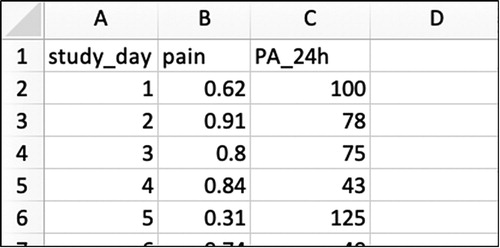
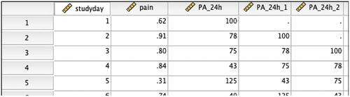
The example data file has all the information needed on the individual of interest. Each variable measured is represented by a column, and each repeated measurement of that variable is represented by a row (see Figure 1 for an example of the Excel worksheet) in what is known as long data format for repeated measures. A variable representing time (e.g. the study day; 1, 2, 3 …) would usually be placed in the first column, followed by the variables defining the outcome (e.g. 24h physical activity), the predictors (e.g. pain) and periodicity (e.g. weekend/workday).

Figure 1. Illustrative example data shown in Excel in the appropriate format for subsequent N-of-1 analyses.

Step 2: identify and impute missing data

Missing data must be identified and imputed (i.e. replaced) in the dataset prior to statistical analysis. Missing data can bias the results of the study as this will affect estimates of autocorrelation. The approach to dealing with missing data should be guided by the degree of missing data; if missing data is minimal (i.e. <10%), a simple imputation rule (e.g. using the mean/median of adjacent data points) may be appropriate, but if the proportion of missing data is substantial, more rigorous procedures for imputation, like multiple imputation, are required (see Schafer & Graham, 2002). Imputing time series data is a serious consideration since imputing data will have an influence on the autocorrelation structure within the data (Velicer & Colby, 2005). Nevertheless, when the amount of missing data is extremely low, it is unlikely to have major implications. In this illustrative example, missing data was minimal (6%) and a simple imputation rule was used (the mean value of the three previous and three subsequent data points). We typically use simple imputation when there is <10% missing data, but methods for addressing missing data in N-of-1 studies is an under-explored area; there are no studies comparing the performance of simple versus multiple imputation at different levels of missingness and thresholds for missing data are largely based on ‘rules of thumb’. In the absence of a consensus on how to address missingness, it is important to at least explicitly describe the amount and type (i.e. missing at random or not) of missing data when reporting the findings from N-of-1 studies. While strategies exist for multiple imputation (e.g. TSimpute, AMELIA II, Forecast; Moritz, Sardá, Bartz-Beielstein, Zaefferer, & Stork, 2015) their discussion is beyond the scope of this paper (see Hobbs et al. (2013) and Quinn et al. (2013) for an example of N-of-1 studies using multiple imputation procedures for missing data).

Step 3: plot the data

Once the dataset has been appropriately formatted and missing data has been addressed, import the data into SPSS, and plot the data over time to allow visual inspection). To plot time series data using SPSS:

• Select Analyze > Forecasting > Sequence charts

• Add the variables of interest into the ‘Variables’ box (see Figure 2)

• Add the variable that represents time (e.g. study_day) into the ‘Time Axis Labels’ box

• If the scale of the variables differs, click the ‘One chart per variable’ box

• Click ‘OK’

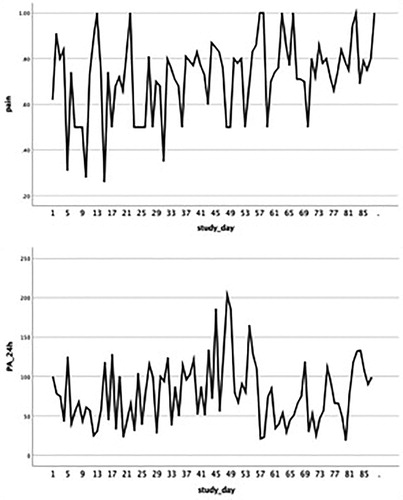
The time plots produced by SPSS are displayed in Figure 3. It is important to inspect these time plots to ensure the measured variables vary sufficiently over time. In this specific example, the pain score varies between 0.20 (mild pain) and 1.00 (extreme pain). However, the outcome would not be as informative if the pain score varied between a smaller range representing e.g. only severe/extreme pain (0.8–1.0) or moderate pain (0.4–0.6). Defining ‘sufficient variability’ is directly related to the research question and the aim of the analysis. If one or more of the measured variables does not vary over time, the ability to detect relationships with other variables will be limited. Visual inspection also provides preliminary information regarding time-related patterns that may exist in the data and possible associations between the outcome and predictors.

Figure 2. Menu options for plotting time series data in SPSS.

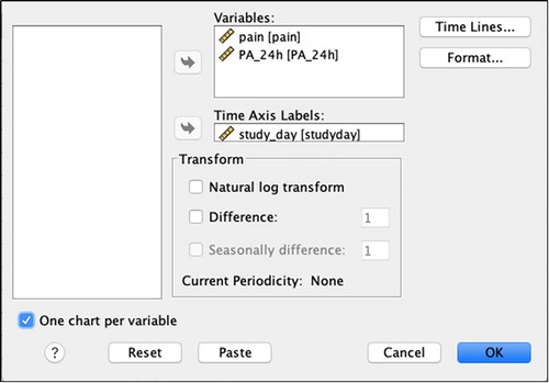
Figure 3. Time plots, produced by SPSS, displaying daily pain and physical activity over the study period.

Step 4: assess the stationarity of the data

A ‘stationary’ time series is when the statistical properties such as mean, variance, autocorrelation, etc. are all constant over time for the outcome variable, and, like most statistical forecasting methods, dynamic regression modelling also relies on the assumption that the time series is approximately stationary. A simple method to check stationarity is to partition the time-series and calculate mean and variance for each partition and see if it changes considerably over time. In this example the time-series is divided into two equally-sized partitions by creating a new variable that identifies each partition. More than two partitions could be used, especially for longer time-series. To partition the data in SPSS and create the necessary descriptives:

• Create variable ‘Partition’ (code: ‘1’ if study_day is less than 45, corresponding to partition 1; ‘2’ if study_day equals or is more than 45, corresponding to partition 2)

• Select Data > Split file > Organise output by groups

• Add the variable ‘Partition’ into the ‘Groups based on’ box

• Click ‘OK’.

• Select Analyze > Descriptive Statistics > Descriptives

• Add the variables of interest (PA_24h) into the ‘Variables’ box

• Click ‘OK’.

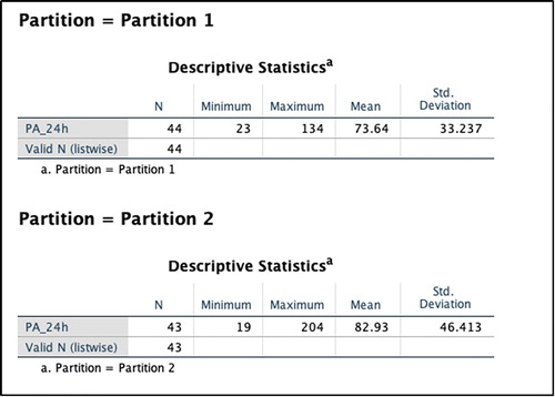
In this illustrative example, the average number of PA minutes in the first partition of the time series is lower by almost 10 min (see Figure 4). Next, potential sources of non-stationarity are investigated.

Figure 4. Output after partitioning the data.

Time trends and periodicity patterns are the most common causes of non-stationarity and de-trending the time-series and/or adjusting for periodicity are usually the next steps in order to deal with non-stationarity. The investigator must remember to reverse the partitioning of the data before continuing with the analysis (Data > Split file > Organise output by groups > Click ‘Analyze all cases, do not create groups’ > Click ‘OK’).

Assessing time trends

The next step involves assessing whether there are any trends in the outcome variable over time (see Figure 5). First, fit a standard linear regression model in SPSS:

• Analyze > Regression > Curve Estimation

• Add the variable ‘PA_24h’ into the ‘Dependent(s)’ box and ‘study_day’ into the Independent ‘Variable’ box.

• Select ‘Plot models’ and ‘Linear’

• Click ‘OK’.

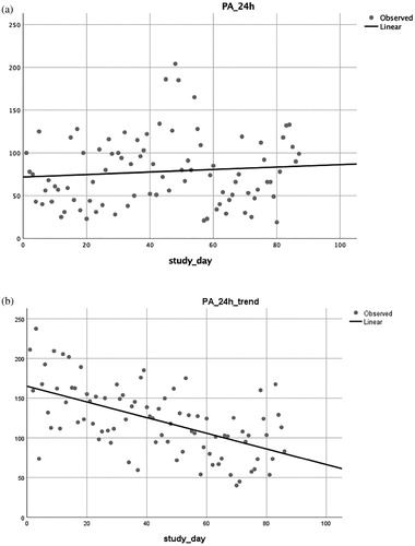
The SPSS output gives the R² of the model (R²= 0.008) assuming a linear relationship between the outcome (PA_24h) and the independent variable (linear time trend), which indicates that this specific variable explains very little of the variability in the data. When looking at the scatterplot (Figure 6a), the time-series dispersion seems fairly stable over time indicating possible non-existence of a trend. Non-linear transformations of the data can be also assessed by following the same steps but selecting non-linear scenarios (e.g. quadratic, cubic, logarithmic, logistic, exponential). In this illustrative example, the model fit was also not improved by any of the above-mentioned non-linear transformations. Therefore, we conclude that there is no evidence of a trend over time in the data from the 87-day study. If a significant linear or non-linear time trend was identified, the time variable would be included in the final regression model. For comparison purposes, Figure 6b displays a scatterplot for data containing a significant linear time trend in physical activity PA, with a decrease in physical activity over time.

Figure 5. Menu options for regressing the outcome variable on the predictor variable(s) to identify whether a linear time trend exists in the data.

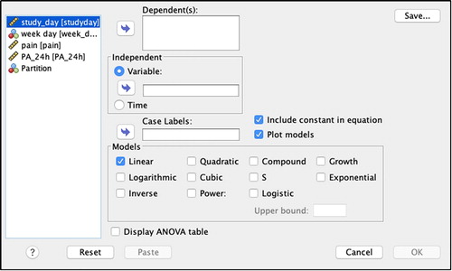
Figure 6. (a) Scatterplot showing stable time-series dispersion indicating possible non-existence of a trend. (b) Scatterplot showing a significant linear time trend in PA, with a decrease in PA over time (for comparison purposes).

Assessing periodic patterns

Time series data may contain periodic variation which translates into cycles that repeat regularly over time. There are many types of periodicity; for example, time of day, daily, weekly, weather seasons, and so on. Once periodicity is identified, it can be modelled. In this illustrative example, it is suspected that there may be an association between minutes of physical activity and whether it is a workday or weekend. The existence of a pattern can be assessed by fitting a standard linear regression model in SPSS:

• Select Analyze > Regression > Linear

• Add the outcome variable (PA_24 h) to the ‘Dependent’ box

• Add the predictor variable (week_day) into the ‘Independent(s)’ box.

• Click ‘OK’

There is no evidence of periodicity in the data as the 95% confidence interval includes 0 and, therefore, this variable will not be included in the final model.

Step 5: check for autocorrelation in the outcome variable

Autocorrelation can be addressed as an integral part of a dynamic regression model and an important concept when characterising autocorrelation is the lag. The lag number represents the interval between data points, e.g. lag1 refers to the immediately preceding data point, lag2 to two data points before, and so on. When theory suggests that some effects operate at a particular lag (e.g. previous day or weekly), the number of lagged variables to be included in the model and respective lags should be chosen accordingly. When no previous knowledge exists, certain algorithmic tools are useful to guide the researcher in making such decisions. However, these tools should be used carefully as data-based algorithms fail to account for the clinical/psychological perspective and can lead to over interpretation of the data. To investigate the presence of autocorrelation in the outcome variable using SPSS:

• Select Analyze > Forecasting > Autocorrelations

• Add the outcome variable (PA_24 h) into the ‘Variables’ box.

• Check the ‘Autocorrelations’ and ‘Partial autocorrelations’ boxes

• Click ‘OK’.

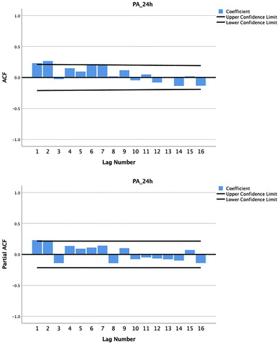
The output will display two correlograms; one with the autocorrelation function (ACF) and one with the partial autocorrelation function (PACF). Firstly, we should examine the sample ACF, which provides the correlation between the consecutive values of the time-series. If any of the bars exceed the 95% confidence limit it indicates that autocorrelation is present and needs to be controlled. The question now is which lags should be included in the model in order to control autocorrelation? The sample PACF provides this information as it shows if any autocorrelation remains at a specific lag, if we were to include all previous lags in the model. The point on the plot where the partial autocorrelations essentially become zero is a good indicator of how many lags should be included. The lags where significant partial autocorrelation is identified should almost certainly be included in the regression model by creating new ‘lagged’ variables, which are added to the model along with the original outcome variable. In Figure 7, the PACF produced from this illustrative example shows that the autocorrelations for lag1 and lag2 are outside the bounds of the 95% confidence interval. According to Box et al. (1994), lags larger than two are rarely required. However, there may be weekly (i.e. represented by lag7 if measurements are daily) or other cyclical autocorrelation structures in the data, which can be identified from the PACF.

Figure 7. Autocorrelation and partial autocorrelation correlograms for physical activity, produced by SPSS.

Step 6: create lagged variables

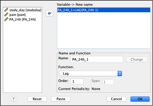
After identifying the autocorrelation structure in step 5, the outcome variable should be lagged accordingly before fitting the regression model (see Figure 8). To create a lagged variable using SPSS:

• Select Transform > Create Time Series

• Select the ‘Function’ dropdown menu and select ‘Lag’ (see Figure 6)

• Add the variable of interest (PA_24h) into the Variable ‘New name’ box.

• Enter ‘1’ into the ‘Order’ box

• Click ‘OK’.

Figure 8. Menu options for creating a lagged variable.

Based on the number of lags identified in the previous step, repeat the above for all lag structures, changing the ‘Order’ number to match the lag value (e.g. for the illustrative example study, this was done for lag1, then lag2). Note that when repeating the above steps for lag2, before clicking ‘OK’, the investigator will need to:

• Amend the ‘Name’ field so that is it unique (e.g. by adding the suffix ‘_2’)

• Click ‘Change’

• Click ‘OK’

The SPSS database will now include new lagged variables (e.g. in the illustrative example dataset, lag1 physical activity is represented by ‘PA_24h_1’; see Figure 9).

Figure 9. New lag1 outcome variable created in SPSS (‘PA_24h_1’).

Step 7: confirm that autocorrelation has been adequately specified

It is important to check that the autocorrelation structure identified in step 5 has been adequately specified, by entering the lagged variables created at step 6 into a regression model, and checking the residuals to ensure they resemble ‘white noise’ (i.e. there is no remaining autocorrelation). To check that autocorrelation has been adequately specified using SPSS:

• Select Analyze > Regression > Linear

• Add the outcome variable (PA_24h) into the ‘Dependent’ box

• Add all lagged outcome variables (PA_24h_1, PA_24h_2) into the ‘Independents(s)’ box

• Click ‘Save’ and select the ‘Unstandardised’ checkbox under ‘Residuals’. Click ‘Continue’

• Click ‘OK’

This will create a residual variable (RES_1) in the SPSS dataset that can be examined for autocorrelation. There should be no significant autocorrelation at any lag in the ACF and PACF for this variable:

• Select Analyze > Forecasting > Autocorrelations

• Add the residual variable (which will be named ‘RES_1’ by SPSS) into the ‘Variables’ box

• Check the ‘Autocorrelations’ and ‘Partial autocorrelations’ boxes

• Click ‘OK’

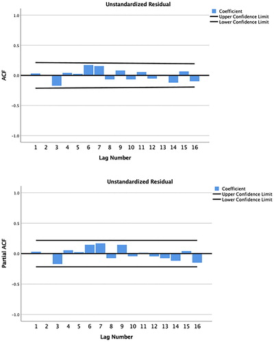
In the data from the illustrative example study, there is no remaining significant autocorrelation in the residuals after including lag1 and lag2 in the regression model (see Figure 10).

Figure 10. Autocorrelation and partial autocorrelation correlograms for physical activity, produced by SPSS.

So far, this analysis covered autocorrelation in the outcome but autocorrelation might also be present in the predictor (yesterday’s pain might be correlated with today’s pain) as well as correlation between today’s outcome (PA) and past pain (e.g. a severe episode of pain might affect PA for several days). In this illustrative example, lagged predictors can be added to the regression model to adjust for such effects. Steps 5–7 could be repeated using the pain variable instead, in order to check for the presence of autocorrelation in the predictor variable. In this specific example, all the bars in the ACF were within the 95% confidence limits which suggests a non-significant amount of autocorrelation. The effect of the past lags of the predictor (e.g. lag1 and lag2 of pain) on the outcome (e.g. physical activity) can be checked in SPSS using linear regression:

• Select Analyze > Regression > Linear

• Add the outcome variable (PA_24h) into the ‘Dependent’ box

• Add all lagged outcome variables (pain_1, pain_2) into the ‘Independents(s)’ box

• Click ‘OK’

In this illustrative example, there is no evidence of such effects, as the 95% confidence intervals for both lags include 0 and, therefore, the lagged predictors will not be included in the final model.

Step 8: conduct dynamic regression analysis

The lagged outcome variables are entered into the regression model along with predictor(s) to identify whether a significant relationship exists between the predictor and the outcome, while accounting for any autocorrelation. To conduct dynamic regression analysis using SPSS:

• Select Analyze > Regression > Linear

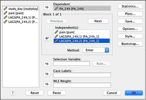
• Add the outcome variable (PA_24h) into the ‘Dependent’ box (see Figure 11)

• Add the predictor variable(s), including the newly created lagged variable(s), into the ‘Independent(s)’ box. If significant time trend, periodic patterns or lagged predictors were identified throughout the process, enter the respective variables into the ‘Independent(s)’ box as well

• Click ‘Statistics’ and select the following checkboxes: ‘Descriptives’ and ‘Confidence intervals’. Click ‘Continue’

• Click ‘Plots’, add ‘*ZRESID’ in the ‘Y:’ box and * ZPRED’ in the ‘X:’ box and select the checkboxes for ‘Histogram’ and ‘Normal probability plot’

• Click ‘Save’ and select the ‘Unstandardised’ checkbox under ‘Residuals’. Click ‘Continue’

• Click ‘OK’

Figure 11. Menu option for entering lagged variables as predictor variables, to control for autocorrelation at the appropriate lag(s).

Step 9: interpret the regression output

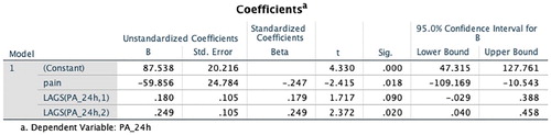
The output from the regression will include, among others, a table providing the mean, standard deviation and number of repeated measures for all variables in the model (Descriptive Statistics), the correlations among all variables (Correlations) and the regression coefficients with the respective 95% confidence intervals (Coefficients and Residual Statistics). In this illustrative example, the regression coefficient is −59.9 and the 95% confidence interval for pain (95%CI: −109.2, −10.5) does not contain zero (Figure 12), indicating that increasing pain is a significant predictor of decreased physical activity in the subsequent 24 hours for this individual. Since dynamic regression modelling is based on conventional regression modelling, it is important to conduct a post-model check to determine whether the usual assumptions of ordinary least squares regression (e.g. linearity, normality, heteroskedasticity) also apply. These can be checked using standard tools such as a histogram and normal probability plot of the residuals and a scatterplot of the residuals versus the predicted values. These were produced at the end of the output in this illustrative example and the assumptions were valid for the final model.

Figure 12. Dynamic regression results – Coefficients table from SPSS.

When the dataset includes data from more than one participant, the data for all participants should be in long format and be uniquely identified using an ID column. To perform separate analyses for all individuals simultaneously in SPSS:

• Select Data > Split file > Organise output by groups

• Add the variable ‘ID’ into the ‘Groups based on’ box

• Click ‘OK’.

However, as a series of decisions will be made throughout the analysis that might impact on what to include in the final model, some steps might still have to be performed separately for each individual.

Step 10: report the results

When reporting the results of an N-of-1 observational study, we recommend reporting the results in the same order as the steps outlined in this tutorial paper. First describe the missing data identified and the procedure used to impute missing data, then present descriptives for each variable (e.g. mean, SD), time plot graphs showing the variation in the outcome over time, any evidence of time-trends or periodicity, the autocorrelation structure identified and used to create lagged variables, and the estimated effect size (regression coefficient) and its precision (such as 95% confidence interval).

The value of N-of-1 observational studies in health psychology and behavioural medicine

Having powerful yet user-friendly statistical methods available for the analysis of N-of-1 observational data will become increasingly important as the role of N-of-1 methods in health psychology and behavioural medicine grows. N-of-1 observational studies provide a novel opportunity to examine relationships between variables at the individual level, which means they are well-suited to testing behavioural theories. Previously, N-of-1 studies have shown that behavioural theories commonly used in health psychology and behavioural medicine, such as the Theory of Planned Behaviour (Ajzen, 1991), may not be valid at the individual level (Hobbs et al., 2013; Quinn et al., 2013). N-of-1 observational methods provide an opportunity to identify temporal relationships between variables due to the time ordered nature of the data (Hobbs et al., 2013), which is not possible using other research designs. For example, relationships between health-related cognitions and later behaviour can provide important information for interventions targeting behaviour change. A major weakness of observational studies is, of course, that such studies cannot establish causality which requires experimental manipulation of the independent variable. However, this can be done in either independent experimental studies or by using the data from the N-of-1 observational study to design a personalised intervention. A good example would be to use a participant’s own empirical data from an N-of-1 observational study to design an intervention that targets the unique determinants of their behaviour, which can then be evaluated in future N-of-1 experimental studies (e.g. O'Brien et al., 2016).

N-of-1 designs are flexible, allowing the opportunity for patient-centred studies where the design of each N-of-1 study is personalised to the unique interests, needs and preferences of the individual (McDonald, Vieira, et al., 2017). N-of-1 observational studies can provide novel insights about an individual that can be used to promote health outcomes, and can ultimately empower individuals to take an active role in their own health (Adler et al., 2016; Nikles, Clavarino, & Del Mar, 2005; Whitney et al., 2018).

Conclusion

This tutorial article introduced readers to the key features of N-of-1 data (i.e. trends, periodic patterns and autocorrelation), which are not likely to feature in traditional statistical education and training in health psychology and behavioural medicine. A 10-step procedure for the analysis of N-of-1 observational data using an approachable but powerful statistical technique performed in a commonly used statistical programme was described. We hope this tutorial article fosters increased awareness, knowledge and skills in relation to the statistical analysis of N-of-1 observational data and sparks further enthusiasm for adding N-of-1 designs to the methodological toolbox in health psychology and behavioural medicine.

Further reading/resources

1. McDonald, Quinn, et al. (2017). The state of the art and future opportunities for using longitudinal n-of-1 methods in health behaviour research: a systematic literature overview, Health Psychology Review, 11, 307–23.

2. McDonald, Vieira, et al. (2017). Dynamic modelling of n-of-1 data: Powerful and flexible data analytics applied to individualised studies, Health Psychology Review, 11, 222–234.

3. The UK Network for N-of-1 Methods. Formed in 2017, this network represents a group of individuals who have an interest in the design, conduct and analysis of n-of-1 studies in health-related research. To join the network, visit: https://uknof1methods.wixsite.com/home

Acknowledgements

We wish to thank Jacelle Warren (The University of Queensland, Australia) for helpful comments on an earlier draft of this tutorial article. We also wish to thank the participant who provided the data used in the illustrative example.

Disclosure statement

No potential conflict of interest was reported by the authors.

Data availability statement

The SPSS dataset and syntax are available within the supplementary materials.

Additional information

Funding

Funding from the Menzies Centre for Australian Studies, King’s College London, University of London (Bicentennial Fellowship Award) awarded to SM to support the conduct of the study described in this tutorial article is gratefully acknowledged.

Notes

1 Approval for the study was obtained from the Medicine Faculty Low and Negligible Risk Sub-Committee at The University of Queensland, Brisbane, Australia

References

- Adler, J., Saeed, S. A., Eslick, I. S., Provost, L., Margolis, P. A., & Kaplan, H. C. (2016). Appreciating the nuance of daily symptom variation to individualize patient care. EGEMS (Wash DC), 4(1), 1247.
- Ajzen, I. (1991). The theory of planned behavior. Organizational Behavior and Human Decision Processes, 50(2), 179–211. doi:10.1016/0749-5978(91)90020-T.
- Araujo, A., Julious, S., & Senn, S. (2016). Understanding variation in sets of N-of-1 trials. PLoS One, 11(12), e0167167. doi: 10.1371/journal.pone.0167167
- Barlow, D. H., Nock, M., & Hersen, M. (2009). Single case experimental designs: Strategies for studying behavior for change (3rd ed.). Boston, London, MA: Allyn and Bacon.
- Bentley, K. H., Kleiman, E. M., Elliott, G., Huffman, J. C., & Nock, M. K. (2018). Real-time monitoring technology in single-case experimental design research: Opportunities and challenges. Behav Res Ther, 117, 87–96. doi: 10.1016/j.brat.2018.11.017
- Blackston, J. W., Chapple, A. G., McGree, J. M., McDonald, S., & Nikles, J. (2019). Comparison of aggregated N-of-1 trials with parallel and crossover randomized controlled trials using simulation studies. Healthcare (Basel), 7(4), 137. doi: 10.3390/healthcare7040137
- Box, G. E. P., Jenkins, G. M., & Reinsel, G. C. (1994). Time series analysis: Forecasting and control (3rd ed.). Englewood Cliffs: Prentice Hall. London: Prentice-Hall International.
- Breiman, L. (2001). Random forests. Journal of Machine Learning, 45(1), 5–32. doi: 10.1023/A:1010933404324
- Burg, M. M., Schwartz, J. E., Kronish, I. M., Diaz, K. M., Alcantara, C., Duer-Hefele, J., & Davidson, K. W. (2017). Does stress result in you exercising less? Or does exercising result in You being less stressed? Or is it both? Testing the Bi-directional stress-exercise association at the group and person (N of 1) level. Annals of Behavioral Medicine, 51(6), 799–809. doi: 10.1007/s12160-017-9902-4
- Davidson, K. W., & Cheung, Y. K. (2017). Envisioning a future for precision health psychology: Innovative applied statistical approaches to N-of-1 studies. Health Psychology Review, 11(3), 292–294. doi: 10.1080/17437199.2017.1347514
- Hobbs, N., Dixon, D., Johnston, M., & Howie, K. (2013). Can the theory of planned behaviour predict the physical activity behaviour of individuals? Psychology & Health, 28(3), 234–249. doi: 10.1080/08870446.2012.716838
- Johnston, D. W. (2016). Ecological momentary assessment. In Y. Benyamini, M. Johnston, & E. Karademas (Eds.), Assessment in health psychology (pp. 241–251). Hogrefe Publishing.
- Johnston, D. W., & Johnston, M. (2013). Useful theories should apply to individuals. British Journal of Health Psychology, 18(3), 469–473. doi: 10.1111/bjhp.12049
- Kazdin, A. E. (1982). Single-case research designs: Methods for clinical and applied settings New York. Oxford: Oxford University Press.
- Kazdin, A. E. (2011). Single-case research designs: Methods for clinical and applied settings (2nd ed.). New York: Oxford University Press.
- Keele, L., & Kelly, N. J. (2006). Dynamic models for dynamic theories: The ins and outs of lagged dependent variables. Political Analysis, 14(2), 186–205. doi: 10.1093/pan/mpj006
- Kratochwill, T. R. (1978). Single subject research: Strategies for evaluating change. New York; London: Academic Press.
- Kravitz, R. (2016). and the DEcIDE methods center N-of-1 guidance panel (Duan N, Eslick I, Gabler NB, Kaplan HC, Kravitz RL, Larson EB, Pace WD, Schmid CH, Sim I, Vohra S). Design and implementation of N-of-1 trials: a user’s guide. AHRQ Publication No. 13 (14)-EHC122-EF. Rockville, MD: Agency for Healthcare Research and Quality; January 2014.
- Kwasnicka, D., & Naughton, F. (2019). N-of-1 methods: A practical guide to exploring trajectories of behaviour change and designing precision behaviour change interventions. Psychology of Sport & Exercise, 101570. doi: 10.1016/j.psychsport.2019.101570
- Manolov, R., Gast, D. L., Perdices, M., & Evans, J. J. (2014). Single-case experimental designs: Reflections on conduct and analysis. Neuropsychological Rehabilitation, 24(3-4), 634–660. doi: 10.1080/09602011.2014.903199
- McDonald, S., & Johnston, D. W. (2019). Exploring the contributions of n-of-1 methods to health psychology research and practice. Health Psychology Update, 26, 38–39.
- McDonald, S., Quinn, F., Vieira, R., O'Brien, N., White, M., Johnston, D. W., & Sniehotta, F. F. (2017). The state of the art and future opportunities for using longitudinal n-of-1 methods in health behaviour research: A systematic literature overview. Health Psychology Review, 11(4), 307–323. doi: 10.1080/17437199.2017.1316672
- McDonald, S., Vieira, R., Godfrey, A., O'Brien, N., White, M., & Sniehotta, F. F. (2017). Changes in physical activity during the retirement transition: A series of novel n-of-1 natural experiments. The international Journal of Behavioral Nutrition and Physical Activity, 14(1), 167. doi: 10.1186/s12966-017-0623-7
- Medical Research Council. (2008). Developing and evaluating complex interventions: new guidance. Retrieved from https://www.mrc.ac.uk/documents/pdf/complex-interventions-guidance/.
- Mengerson, K., McGree, J., & Schmid, C. H. (2015). Statistical analysis of n-of-1 trials. In J. Nikles, & G. Mitchell (Eds.), The essential guide to N-of-1 trials in health (pp. 135–153). Netherlands: Springer.
- Moritz, S., Sardá, A., Bartz-Beielstein, T., Zaefferer, M., & Stork, J. (2015). Comparison of different methods for univariate time series imputation in R. arXiv preprint, p arXiv:1510.03924.
- Nikles, C. J., Clavarino, A. M., & Del Mar, C. B. (2005). Using n-of-1 trials as a clinical tool to improve prescribing. The British Journal of General Practice, 55(512), 175–180.
- Ninci, J., Vannest, K. J., Willson, V., & Zhang, N. (2015). Interrater agreement between visual analysts of single-case data: A meta-analysis. Behavior Modification, 39(4), 510–541. doi: 10.1177/0145445515581327
- O'Brien, N., Philpott-Morgan, S., & Dixon, D. (2016). Using impairment and cognitions to predict walking in osteoarthritis: A series of n-of-1 studies with an individually tailored, data-driven intervention. British Journal of Health Psychology, 21(1), 52–70. doi: 10.1111/bjhp.12153
- Quinn, F., Johnston, M., & Johnston, D. W. (2013). Testing an integrated behavioural and biomedical model of disability in N-of-1 studies with chronic pain. Psychology & Health, 28(12), 1391–1406. doi: 10.1080/08870446.2013.814773
- R Core Team. (2018). R: A language and environment for statistical computing. Vienna, Austria: R Foundation for Statistical Computing. Retrieved from https://www.R-project.org/
- Sainsbury, K., Vieira, R., Walburn, J., Sniehotta, F. F., Sarkany, R., Weinman, J., & Araujo-Soares, V. (2018). Understanding and predicting a complex behavior using n-of-1 methods: Photoprotection in xeroderma pigmentosum. Health Psychology, 37(12), 1145–1158. doi: 10.1037/hea0000673
- Schafer, J. L., & Graham, J. W. (2002). Missing data: Our view of the state of the art. Psychological Methods, 7(2), 147–177. doi: 10.1037/1082-989X.7.2.147
- Schmid, C. H. (2001). Marginal and dynamic regression models for longitudinal data. Statistics in Medicine, 20(21), 3295–3311. doi: 10.1002/sim.950
- Shadish, W. R., Kyse, E. N., & Rindskopf, D. M. (2013). Analyzing data from single-case designs using multilevel models: New applications and some agenda items for future research. Psychological Methods, 18(3), 385–405. doi: 10.1037/a0032964
- Shiffman, S., Stone, A. A., & Hufford, M. R. (2008). Ecological momentary assessment. Annual Review of Clinical Psychology, 4, 1–32. doi: 10.1146/annurev.clinpsy.3.022806.091415
- Smith, J. D. (2012). Single-case experimental designs: A systematic review of published research and current standards. Psychological Methods, 17(4), 510–550. doi: 10.1037/a0029312
- Smith, G., Williams, L., O'Donnell, C., & McKechnie, J. (2018). A series of n-of-1 studies examining the interrelationships between social cognitive theory constructs and physical activity behaviour within individuals. Psychology & Health, 34(3), 1–16.
- Tate, R. L., Perdices, M., Rosenkoetter, U., Shadish, W., Vohra, S., Barlow, D. H., … Wilson, B. (2016). The single-case reporting guideline In behavioural interventions (SCRIBE) 2016 Statement. Journal of Clinical Epidemiology, 73, 142–152. doi: 10.1016/j.jclinepi.2016.04.006
- Tate, R. L., Perdices, M., Rosenkoetter, U., Wakim, D., Godbee, K., Togher, L., & McDonald, S. (2013). Revision of a method quality rating scale for single-case experimental designs and n-of-1 trials: The 15-item risk of bias in N-of-1 trials (RoBiNT) scale. Neuropsychological Rehabilitation, 23(5), 619–638. doi: 10.1080/09602011.2013.824383
- Velicer, W. F., & Colby, S. M. (2005). A comparison of missing-data procedures for ARIMA time-series analysis. Educational and Psychological Measurement, 65(4), 596–615. doi: 10.1177/0013164404272502
- Vieira, R., McDonald, S., Araujo-Soares, V., Sniehotta, F. F., & Henderson, R. (2017). Dynamic modelling of n-of-1 data: Powerful and flexible data analytics applied to individualised studies. Health Psychology Review, 11(3), 222–234. doi: 10.1080/17437199.2017.1343680
- Vohra, S., Shamseer, L., Sampson, M., Bukutu, C., Schmid, C. H., Tate, R., … Group, C. (2015). CONSORT extension for reporting N-of-1 trials (CENT) 2015 Statement. BMJ, 350, h1738. doi: 10.1136/bmj.h1738
- Whitney, R. L., Ward, D. H., Marois, M. T., Schmid, C. H., Sim, I., & Kravitz, R. L. (2018). Patient perceptions of their own data in mHealth technology-enabled N-of-1 trials for chronic pain: qualitative study. Jmir Mhealth and Uhealth, 6(10), doi: 10.2196/10291
- Zucker, D. R., Ruthazer, R., & Schmid, C. H. (2010). Individual (N-of-1) trials can be combined to give population comparative treatment effect estimates: Methodologic considerations. Journal of Clinical Epidemiology, 63(12), 1312–1323. doi: 10.1016/j.jclinepi.2010.04.020