Antigenicity prediction and vaccine recommendation of human influenza virus A (H3N2) using convolutional neural networks

ABSTRACT

The rapid evolution of influenza A viruses poses a great challenge to vaccine development. Analytical and machine learning models have been applied to facilitate the process of antigenicity determination. In this study, we designed deep convolutional neural networks (CNNs) to predict Influenza antigenicity. Our model is the first that systematically analyzed 566 amino acid properties and 141 amino acid substitution matrices for their predictability. We then optimized the structure of the CNNs using particle swarm optimization. The optimal neural networks outperform other predictive models with a blind validation accuracy of 95.8%. Further, we applied our model to vaccine recommendations in the period 1997 to 2011 and contrasted the performance of previous vaccine recommendations using traditional experimental approaches. The results show that our model outperforms the WHO recommendation and other existing models and could potentially improve the vaccine recommendation process. Our results show that WHO often selects virus strains with small variation from year to year and learns slowly and recovers once coverage dips very low. In contrast, the influenza strains selected via our CNN model can differ quite drastically from year to year and exhibit consistently good coverage. In summary, we have designed a comprehensive computational pipeline for optimizing a CNN in the modeling of Influenza A antigenicity and vaccine recommendation. It is more cost and time-effective when compared to traditional hemagglutination inhibition assay analysis. The modeling framework is flexible and can be adopted to study other type of viruses.

KEYWORDS:

• Convolution neural networks
• Influenza A
• H3N2
• particle swarm optimization
• antigenicity
• machine learning
• deep learning
• flu vaccine strain selection

Significance statement

Influenza A viruses remain dangerous pathogens with the potential to cause pandemic outbreaks. The World Health Organization (WHO) is constantly monitoring the circulation of influenza viruses to detect potential pandemic strains. And each year, WHO recommends which strains should be included in the flu vaccine to protect people from seasonal flu. We apply a state-of-the-art deep learning approach to tackle this problem. Our study designs an in-silico prediction of antigenicity of Influenza A virus using convolutional neural networks. We systematically analyze the selection of the physicochemical properties and optimize the structure of the neural networks. This leads to a blind validation accuracy of 95.8%. Further, using our model, we show that vaccine strain recommendations could be improved significantly.

Background

Current state-of-the-art antigenicity models

The genome of Influenza viruses is constantly changing, and thus continuous vigilance is required to protect the world population not only from seasonal influenza but also from novel influenza A viruses that could trigger a pandemic. Seasonal Influenza is an acute viral infection and is estimated to cause 3 to 5 million cases of severe illness and around 250,000 to 500,000 deaths worldwide.¹ Among the three subtypes, type A is the only one known to cause pandemics.¹

Vaccination is the most effective way to prevent Influenza outbreaks and epidemics. To produce a qualified vaccine, a composition virus must be evaluated and should represent the newly emerged circulating virus which escaped from the immune system of the human body. However, the rapid evolution of influenza virus poses a severe challenge for fast and accurate vaccine production.² Modeling of Influenza pathogenicity has focused on Hemagglutinin (HA) which executes the function of binding with host cells and triggers the process of virus internalization.³ Hemagglutinin is also the primary target of antibodies. Two mechanisms have empowered HA with the capability of frequent escape from the elimination of the human immune system, one is antigenic drift due to lack of proof-reading of RNA polymerase,⁴ the other is reassortment of one or more gene segments.^5,6

The “gold standard” for evaluating the efficacy of vaccine and characterization of virus strains is the hemagglutination inhibition assay (HAI assay).^7,8 However, the process of conducting HAI assay is labor and cost intensive. Hence, a wide range of sequence-based methods have been proposed to infer the antigenicity of new Influenza virus.^9–14

Numerous research efforts^13,15–18 have explored point mutations and their association of influenza epidemic, based on a limited number of amino acid properties. However, these models only measure the contribution of chosen amino acids as individuals. Thus, they lack the context that changes of amino acids in HA may have composite effects since they form a 3D structure in space.

There are several promising approaches. YC Liao¹² improved the model by quantifying the amino acid difference with change of polarity, charge and structure; and applied an iterative filtering algorithm, multiple regression, logistic regression and support vector machine (SVM) algorithms. Y Yao¹¹ observed the limitation in the selection of amino acid matrices in previous sequence-based methods and systematically analyzed amino acid index dataset 2. And J Qiu¹⁹ stepped beyond sequence information by incorporating spatial information with a linear model.

Understanding the combinatorial effect of point mutations of Influenza A and expanding the number of amino acids in the analysis may better unveil the relationship between HA sequence and its antigenicity. In this study, we designed a computational pipeline based on CNN and fast optimization algorithms for antigenicity prediction. Our model is the first that explores systematically all the amino acids and their combinatorial effect. We benchmarked our system-CNN approach with current state-of-the-art methodologies.^11,12,19

We also demonstrated our approach in finding optimal strains for vaccination recommendation and established a pipeline for a highly reliable and efficient recommending system. A reliable prediction of antigenicity can be readily applied to vaccine composition recommendation. Influenza A virus is continuously monitored globally, and twice yearly WHO work in collaboration with experts from WHO Collaborating Centers and Essential Regulatory Laboratories to make recommendations on influenza vaccine composition for both the northern and southern hemispheres for the next epidemic season. A successful selection of vaccine strain is signified by highly induced immune effect against the target virus, which requires the chosen vaccine representing the new mutations of the current circulating virus. The selection of vaccine strain involves the collection of clinical specimens, diagnosis and virus isolation, antisera production, thorough antigenic and genetic analysis, serological study of seasonal influenza vaccine and finally the selection of candidate viruses for vaccine use.²⁰ The antigenic and genetic analysis process is primarily composed of continuous HAI assay test, in which candidate strains are tested against circulating ones and the “antigenic distance” is measured. However, this traditional methodology is limited by the availability of high-level biosafety laboratories and economic cost. Our in-silico computational model analyzes all potential amino acids and combinatorial properties and returns a promising vaccine recommendation that outperforms the current WHO vaccine recommendation and other existing models. The pipeline is cost-effective, evidence-based and can be adaptable for other viral analysis.

Application of convolutional neural network

Deep convolutional neural network (CNN) has been applied successfully in visual analysis^21–24 and natural language processing.^25–27 A CNN is usually composed of one or more convolutional layers. However, instead of each neuron in one layer being connected to all neurons in the next layer, regularization of CNNs takes advantage of the hierarchical pattern in data and assembles more complex patterns using smaller and simpler patterns. Therefore, on the scale of connectedness and complexity, CNNs are on the lower extreme.

Each convolutional layer scans through the input and generalizes higher level characteristics of the input. The process starts by choosing a filter/kernel size and scans the input systematically through a sliding window to identity critical features. This is usually followed by non-linear activation, pooling and dropout. Each convolutional layer may contain multiple kernels, each of which focuses on a specific characteristic of the input, such as edges, corners, diagonal lines, etc. The summarized characteristics can be further used in many applications, such as image classification, and generative models. Appendix 1 includes a simplified example of a CNN and various components.

Given its outstanding performance in image processing, CNN is heavily applied in medicine especially within the realm of cancer detection^28–30 and neurology.^31–33 D Quang³⁴ proposed a hybrid convolutional and recurrent deep neural network to predict the function of non-coding regions of DNA. J Kim³⁵ applied CNN on climate heat maps to detect Influenza outbreaks. S Zhong³⁶ applied CNN to predict Influenza dynamics in a location network for location-oriented intervention strategy. This paper marks the first application of CNN to antigenicity analysis of influenza.

The structural design of a neural network is critical for its performance. Tuning the hyperparameters and structure (e.g., how many convolutional layers, kernel sizes, step size, pooling approach, dropout rates, etc.) of a deep neural network via a manual process requires much expertise and experience and remains a challenge due to the large number of architectural design choices. Numerous approaches have been proposed to optimize the architecture of neural networks.^37–48 Despite their successes, most of them are restricted to a fixed search space and cannot handle non-continuous space. To address this issue, biological inspired algorithms have been applied including particle swarm optimization (PSO)^37,47 and genetic algorithms.^46,48 Among these approaches, PSO is able to optimize the structure, hyperparameters and activation of a neural network simultaneously while maintaining good computational performance.³⁷

Study objective

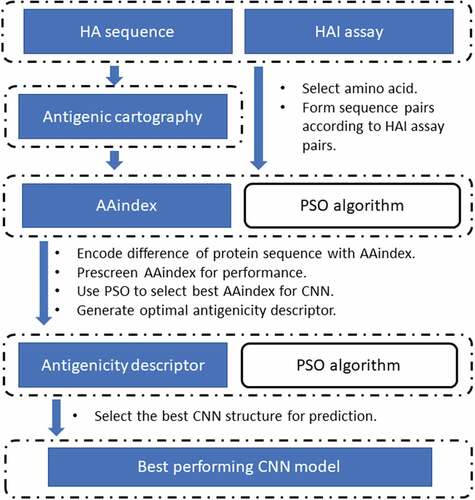
In this study, we designed a systems biology deep learning framework to analyze all prior years’ viruses to predict and select a set of strains for vaccine development. We first evaluated the combinatorial effect of point mutations of Influenza A virus using a CNN approach for antigenicity quantifying (Figure 1). The CNN model was designed to scan a large sub-region of the Influenza sequence, which enables the model to potentially quantify the spatial relationship and interaction of amino acids that are not necessarily adjacent in a sequence. The CNN model extracted and formulated high-level patterns from the sequence through intermedia layers, advancing the understanding of pathogenicity of the virus. We optimized the CNN model and its feature space. The fast PSO heuristic offers an efficient computational environment while achieving good performance in the resulting CNN model.

Figure 1. A computational pipeline for antigenicity prediction. HA sequence and HAI assay data were used to construct HAI sequence pairs. HAI assay was also used to make antigenic cartography to generate more HA pairs (augmented set via multi-dimensional scaling). The HA sequence pairs were filled with data using the metrics in AAindex, the choice of which was optimized using a PSO algorithm. Upon obtaining the optimal antigenicity descriptor, the optimal CNN model is constructed using PSO

Specifically, leveraging CNN’s effectiveness in recognizing patterns in images, we innovatively constructed the patterns of the HA protein sequence using amino acid indices. Training on these patterns, the CNN model analyzed the contributions introduced by individual mutations and their associated combinational effects. Furthermore, we systematically analyzed all available amino acid properties for the predictability of H3N2 antigenicity.

We next applied the predicted antigenicity results to vaccine composition recommendation and contrast our results with existing approaches. Specifically, we first reported the efficacy of the World Health Organization (WHO) vaccine recommendation. Next, we analyzed the ideal scenario: an optimal vaccine recommendation when the circulating strains are known. This was followed by exploring optimal vaccine recommendations using our CNN model.

Materials and methods

This study is composed of six major steps:

1. Collect data from public sources and construct antigenicity cartography,

2. Define antigenic distance and select the threshold for discriminating antigenic variant versus antigenic similar,

3. Select amino acids to represent HAI pairs via evolutional conservation threshold, regression model and information theory,

4. Optimize the selection of AAindex using PSO to obtain the best combinatorial amino acids properties that result in the best prediction accuracy,

5. Optimize the hyperparameters of CNNs via particle swarm heuristics to obtain the best prediction,

6. Determine the vaccine strain recommendation and contrast it with the WHO selection and the optimized “ideal” scenario.

Dataset

HAI assay data were collected and combined from T Bedford⁴⁹ and WHO reports. The T Bedford dataset includes HAI titer for seasonal A/H3N2 influenza viruses and ferret antisera isolated between 1968 and 2011, which has a total of 10,059 recordings of antigen-antiserum pairs. The dataset from WHO was obtained via batch search, weekly epidemiological records, and Influenza summary, covering the period from 1980 to 2017. After filtering for A/H3N2, we obtained a total of 755 HAI titer pairs from these WHO records. Duplicates in the datasets were averaged into one entry and titer numbers indicated as “<20” and “<40” were taken as half of the value. The final set contains 6,166 unique HAI titer pairs. Among the HAI titer data, 5,916 pairs involving virus strains from 1968 to 2010 were used as the training set, while the remaining 250 pairs from 2011 to 2016 were used as an independent blind validation set.

Antigenic Cartography is the process of creating maps of antigenically variable pathogens Using multidimensional scaling proposed by DJ Smith,⁵⁰ we constructed the antigenic cartography and acquired 156,255 HAI pairs calculated using the coordinates of the strains. This augmented dataset supplements the pair-wise relationships between virus and antigenic serum, which were too expensive to acquire via traditional experimental approaches. This augmented set was then partitioned into 145,930 training samples and 10,325 blind validation samples using the same partition time range.

In total, we obtained 463 strains and the HAI protein sequences were downloaded from NCBI Influenza Virus Database,⁵¹ Influenza Research Database⁵² and GISAID.⁵³ The sequences were aligned using MUSCLE⁵⁴ with the default parameters.

Antigenic distance

The HAI titer value $H_{ij}$ is the maximum dilution of serum containing antibody raised against virus $j$, which is necessary to inhibit erythrocytes agglutination induced by virus $i$. We followed Smith’s⁵⁰ definition of antigenic distance:

(1) $D_{ij}=b_j-lo{g}_2\left(H_{ij}\right)$(1)

(2) $b_j=lo{g}_{2}max\left(HAIofantiserumj\right)$(2)

If $D_{ij}$ is greater than 4, virus $i$ and $j$ are considered antigenic variant (positive), otherwise they are antigenic similar (negative). An antigenic variant pair represents that one virus can “escape” from the immune system that was vaccinated by the other virus.

Modeling antigenic variance

Conservation scores were calculated using ConSurf⁵⁵ for the selection of amino acids. Amino acid positions in the alignment with no gaps and a conservation score smaller than 0.99 were collected as the basis for making quantitative descriptors of antigenic variance. A logistic regression model, Equation (3)(3) $y=\frac{1}{1+e^{-\left({\beta }_0+{\beta }_{1}x\right)}}$(3) , was constructed to further filter the candidate amino acids.

(3) $y=\frac{1}{1+e^{-\left({\beta }_0+{\beta }_{1}x\right)}}$(3)

For each amino acid position, a binary vector x was constructed across all HAI pairs which represent the difference between virus and serum. After convergence, the mutual information (MI), Equation ($4$), of predicted and true response was calculated and a threshold of 1e-4 was used to filter the amino acids candidates.

(4) $I\left(X,Y\right)=\sum _{x\in X}\sum _{y\in Y}p\left(x,y\right)log\left(\frac{p\left(x,y\right)}{p\left(x\right)p\left(y\right)}\right)$(4)

Unlike previous studies^11,15,19 which limit the selection of candidate amino acids to surface accessible ones, we considered the potential importance of inner amino acids.

For all the amino acid positions, we constructed a vector corresponding to the HAI titer pairs with the value in the vector deduced from selected amino acid indices⁵⁶ and the representing aligned HA sequences. The value is obtained by subtracting the value of amino acid in serum virus from that of antigen virus. The AAindex database is a flat file database that consists of three sections: AAindex1 for the amino acid indices, AAindex2 for the amino acid substitution matrices and AAindex3 for the amino acid contact potentials. We applied logistic regression to test the predictability of three amino acid indices one at a time. A moving window technique was used to produce 10 training and testing sets based on the year of the virus, thus guaranteeing that older pairs were used to predict the newer pairs. The performance was averaged among the 10 sets.

After comparing both Matthews correlation coefficient (MCC) and MI of the training and testing sets, only AAindex 2 and 3 merited further analysis. Upon filtering out the non-applicable values, we obtained 92 matrices of AAindex 2 and 43 matrices of AAindex 3. We used PSO to further narrow the candidates from these AAindex 2 and 3 matrices.

Convolutional neural networks (CNN)

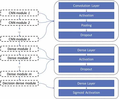
We next implemented the CNN models using Keras v2.0.8.⁵⁷ Our CNN includes the convolution layers, the pooling layers, the dropout layer, and the fully connected layers. A convolution layer is defined by the number of filters, filter size, stride size, and activation function. A pooling layer is defined by the kernel size and stride size. A dropout layer is defined by the probability of dropout. And a fully connected layer is defined by the number of neurons and activation function. Figure 2 illustrates the structure of our CNN model. We formed a vector using the CNN hyperparameters, along with the number of CNN modules and number of dense layers. We normalized it appropriately and then optimized using PSO. Table 1 summarizes the range of hyperparameters used in the CNN model.

Table 1. Range of hyper-parameters used in our CNN

Hyperparameter	Min	Max
Number of CNN modules	1	4
Number of filters	32	256
Filter size	2	5
Filter stride	1	3
Pooling size	1	4
Pooling stride	1	4
Dropout probability	0.1	0.5
Number of dense modules	1	3
Number of neurons in dense layers	72	256
Dropout probability	0.1	0.5

Figure 2. Design schema of our CNN networks

Particle swarm optimization

PSO^58,59 was designed to optimize the choice of amino acid indices, and the structure and the hyperparameters of our CNN model. Our PSO algorithm was implemented in Python 3.6 and worked as follows:

Step 1. Initialize the optimization process with a set of 25 particles with random locations and velocities.

Step 2. Define the von Neumann neighborhood⁶⁰ for the initialized particles.

Step 3. Evaluate the fitness function for each particle. If the fitness value is better than the particle’s best value, update the personal best position ${\mathrm{p}}_{\mathrm{b}\mathrm{e}\mathrm{s}\mathrm{t}}^{\mathrm{p}}$, and the personal best value ${\mathrm{v}}_{\mathrm{b}\mathrm{e}\mathrm{s}\mathrm{t}}^{\mathrm{p}}$ accordingly.

Step 4. Compute the local best value ${\mathrm{v}}_{\mathrm{b}\mathrm{e}\mathrm{s}\mathrm{t}}^{\mathrm{l}}$, local best position ${\mathrm{p}}_{\mathrm{b}\mathrm{e}\mathrm{s}\mathrm{t}}^{\mathrm{l}}$ to update all particles. Change the velocity and position of particles according to the following formula:⁶¹

(5) $v_{t+1}=w\ast v_t+r_1\ast c_1\ast \left(p_{best}^p-p_t^p\right)+r_2\ast c_2\ast \left(p_{best}^l-p_t^p\right)$(5)

(6) $p_{t+1}^p=p_t^p+\Delta t\ast v_{t+1}$(6)

Step 5. Go to Step 3 until the maximum number of iterations is met or the change of global best value is less than a pre-set threshold.

We selected 10 indices from the AAindex. A binary vector was used to represent the selection of the AAindex and served as the position vector of the particles. The PSO algorithm was initialized with 25 particles, and a random speed uniformly initiated between −1 and 1. The algorithm terminates when the maximum number of iterations reaches 50, or when the change in the global best value is smaller than $1e^{-6}$. In the process of updating the particle’s position vector, the top ten ranked elements were set to 1 and the rest to 0, which maintains the conceptual rule of the position vector. The fitness value was returned by a simple CNN model (Table 2), which uses the position vector as the choice of AAindex and trained with 10 epochs and batch size of 600.

Table 2. CNN structure used for optimizing AAindex selection

Layer Index	Layer
1	Convolution; Filter: 32, Filter size: 3, stride: 1, activation: relu.
2	Max pooling; Kernel size: 2, stride: 2.
3	Dropout; Dropout rate: 0.3.
4	Dense; Neurons: 128, activation: relu.
5	Dropout; Dropout rate: 0.5.
6	Dense; Neurons: 64, activation: relu.
7	Dropout; Dropout rate: 0.5.
8	Dense; Neurons: 1, activation: sigmoid.

Upon termination, the optimal position vector was reported and the corresponding AAindex were retrieved. The selected 10 AAindex were then used to calculate the value difference between virus strain and serum strain. The resulting values form the feature matrix for each HAI pair. In the final step, a tensor (size: sample size$\times$amino acid candidates$\times$selected AAindices) was generated and split accordingly for further training and blind validation.

In the optimization of the CNN structure, a vector of length 26 with continuous values ranging between 0 and 1 was used to represent the structure of the underlying CNN. In the optimization process, the constant inertia w is set to 0.5, cognitive constant c₁ and social constant c₂ are both set to 2.

Performance metrics

The performance of the models was evaluated using accuracy, sensitivity, specificity, MCC and f-score on their predictability of antigenic variance. Specifically,

(7) $Accuracy=\frac{TP+TN}{TP+TN+FP+FN}$(7)

(8) $Sensitivity=\frac{TP}{TP+FN}$(8)

(9) $Specificity=\frac{TN}{TN+FP}$(9)

(10) $MCC=\frac{TP\times TN-FP\times FN}{\sqrt{\left(TP+FP\right)\left(TP+FN\right)\left(TN+FP\right)\left(TN+FN\right)}}$(10)

(11) $F-score=2\cdot \frac{precision\cdot recall}{precision+recall}$(11)

where TP represents true positive, TN represents true negative, FP represents false positive and FN represents false negative. We recognize the problem of accuracy/sensitivity/specificity. Our study is guided in part by our CDC collaborators who advise us. This study uses MCC and f-score to compensate for bias.

We also contrasted our model performance with the currently most promising approaches from the literature: YC Liao’s,¹² J Qiu’s¹⁹ and Y Yao’s.¹¹

Optimization of vaccine recommendation

The recommendation of H3N2 vaccine composition was collected from the data repository of WHO, among which we chose six strains for analysis (Table 3).

Table 3. WHO’s recommendation of H3N2 vaccine composition

Strain	Start year	End year
A/Sydney/5/1997	1998	2000
A/Moscow/10/1999	2000	2004
A/Fujian/411/2002	2004	2005
A/California/7/2004	2005	2006
A/Wisconsin/67/2005	2006	2008
A/Brisbane/10/2007	2008	2010

The efficacy of vaccine composition can be measured by antigenicity coverage which is defined as

(12) $C_{a,i}=\frac{K_{a,i}}{M_i}$(12)

Here C_a,i denotes the antigenicity coverage of strain a in year i, K_a,i represents the number of strains similar to strain a in year i, and M_i means the total number of newly emerged vaccine strains in year i.

We proposed the following optimization to obtain the optimal recommendation of vaccine composition: $max{\sum }_{i=1}^{n-1}\left[w\left(s_i|y_i\right)+w(s_{i+1}|y_{i+1})\right]$

(13) $s.t.g\left(s_i\right)<y_i,i=1,\dots ,n$(13)

where g(s_i) represents the year of virus strain s_i, and w(s_i|y_i) is the antigenicity coverage of virus strain s_i in the year of y_i. Constraint (13) restricts the selection of candidate vaccine to emerge earlier than the year of recommendation.

Results

Selection of candidate amino acids

We extend the traditional way of selecting antigenicity-dominant positions from surface ones to all non-conserved amino acids. This was based on two assumptions: 1) Surface amino acids may directly interact with antibodies, and inner amino acids are equally important in the role of affecting the overall 3D structure of the protein; 2) The change of antigenicity introduced by point mutations is more complicated than a linear addition of individual contributions, thus requiring comprehensive modeling of spatial and long distance interactions.

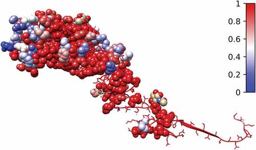
We collected amino acid positions in the alignment of the 463 HAI protein sequences with no gaps and a conservation score smaller than 0.99 as the basis for making quantitative descriptors of antigenic variance. This resulted in a total of 116 most mutated amino acid positions (Figure 3). The number was further reduced to 96 using a MI threshold.

Figure 3. Conservation score calculated using the alignment of all protein sequences and shown on the 3D structure of 3HMG. The 96 selected amino acids are shown as sphere and the rest are shown as ribbon. Red represents the most conserved, and blue represents the most non-conserved

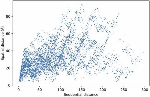
The relationship between spatial and sequential distances of the 96 candidate amino acid positions is explored in Figure 4. We observe that due to the complexity of HA1, the distances are not linearly related. This phenomenon indicates that amino acids on the HA structure can interact even with large sequence distances between them. To facilitate our model to learn this phenomenon, the size of the first kernel of our CNN networks was fixed at 96, equaling the total number of amino acids selected for prediction.

Figure 4. Spatial and sequential distances of candidate amino acids. Each amino acid pair is represented by a dot in the figure. There are 4,560 pairs for the 96 amino acids

Systematic analysis of predictability of AAindex

AAindex⁵⁶ is a database of numerical values representing physicochemical and biochemical properties of single and paired amino acids. AAindex has three sections: amino acid physicochemical properties (AAindex1), substitution matrices (AAindex2) and statistical protein contact potentials (AAindex3). The choice of AAindex is crucial to the predictability of machine learning models.

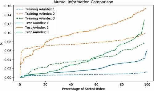
After filtering out missing data in AAindex, we obtained 553, 92, and 43 recordings of AAindex 1, 2, and 3, respectively. Each of the recording was used to construct the feature vector based on the resulting 96 amino acid positions. The predictability measured by MCC and MI was obtained using a simple logistical model (Figures 5 and 6). The sorted MCC and MI slopes of AAindex 2 and 3 indicate sufficient potential in predictability, whereas AAindex 1 does not. The best MCC of training samples using AAindex 2 and 3 reaches as high as 0.465 and 0.409, respectively, while AAindex 1 only achieves 0. This result reflects the fact that AAindex 2 and 3 measure the properties involved in amino acid interaction and interchanging instead of merely the physical and chemical features as in AAindex 1. We then performed the final feature selection step restricted to the sets AAindex 2 and 3.

Figure 5. Comparing Matthews correlation coefficients produced using each of the AAindex as predicting variable via a logistic regression model

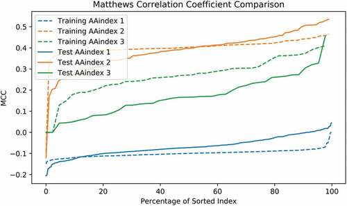
Figure 6. Comparing mutual information produced using each of the AAindex as predicting variable via a logistic regression model

Optimized selection of AAindex

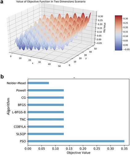
Our analysis showed that PSO is a robust solution engine for selecting the amino acids. We benchmarked several optimization algorithms including Newton’s method, Nelder-Mead,⁶² Powell’s algorithm,⁶³ the Conjugate Gradient method,⁶⁴ the Broyden–Fletcher–Goldfarb–Shanno algorithm (BFGS),⁶⁵ the limited-memory BFGS-B (L-BFGS-B),⁶⁶ the truncated Newton (TNC) algorithm,⁶⁷ constrained optimization by linear approximation (COBYLA),⁶⁸ and sequential least squares Programming (SLSQP).⁶⁹ In a scenario where there are multiple local maxima (Figure 7(a)), the PSO algorithm is able to find the global maximum when other algorithms failed (Figure 7(b)). All these algorithms were trapped in a local maximum which is close to the initial starting point, while the Nelder-Mead algorithm failed to converge.

Figure 7. (a) A scenario with numerous local maxima. (b) Comparison of optimization algorithms on 25 instances

The PSO algorithm returns 10 matrices from AAindex 2 and 3 (Table 4). Our results differ notably from previous findings: the amino acids PAM250 and BLOSUM62 were not selected, although they are commonly thought to have good predictability.^12,70,71 These two matrices were also absent in one previous research result.¹⁶ After ranking the MCC of AAindex candidates using a logistical regression model, it shows that the selected candidates are not merely a collection of best performing single variates. Rather in combination they produce the best results. This is not possible to achieve using a step-wise optimization algorithm.

Table 4. Optimized AAindex for further feature construction

AAindex ID	AAindex Source	Description	Rank
BENS940104	2	Genetic code matrix (Benner et al., 1994)	18
LUTR910108	2	Structure-based comparison table for alpha helix class (Luthy et al., 1991)	53
MUET010101	2	Non-symmetric substitution matrix (SLIM) for detection of homologous transmembrane proteins (Mueller et al., 2001)	63
KOLA920101	2	Conformational similarity weight matrix (Kolaskar-Kulkarni-Kale, 1992)	75
AZAE970101	2	The single residue substitution matrix from interchanges of spatially neighboring residues (Azarya-Sprinzak et al., 1997)	86
BONM030104	3	Distances between centers of interacting side chains in the antiparallel orientation	1
TANS760101	3	Statistical contact potential derived from 25 x-ray protein structures	5
ZHAC000106	3	Environment-dependent residue contact energies (rows = coil, cols = coil)	7
BETM990101	3	Modified version of the Miyazawa-Jernigan transfer energy	22
BONM030103	3	Quasichemical statistical potential for the parallel orientation of interacting side groups	29

Optimized deep neural network structure

An optimized structure of CNN is reported back with three convolutional layers and one fully connected layer (Table 5). The convolutional layers treat the input tensor as an image of size 96*10 with only one channel, and scan through the “image” with specific kernel size and stride steps, which extract and form the upper level features from the previous layer.

Table 5. Optimized structure of convolutional neural network

	Filter/Neurons	Kernel size	Stride	Pooling	Dropout
Conv 1	193	96*10	3	1	0.1
Conv 2	212	5*10	2	1	0.165
Conv 3	109	5*10	3	1	0.1
Dense 1	256	N/A	N/A	N/A	0.241

Performance of the CNN model

We tested our CNN model extensively and validated using two sets of data: the original data set and the augmented set obtained via multi-dimensional scaling. The first data set contains 5,916 HAI pairs for training and 250 for blind validation. This results in a well-balanced positive case ratio of 0.432 and 0.412. The augmented set contains 145,930 for training and 10,325 for blind validation. This augmented dataset results in positive case ratio of 0.780 and 0.923, respectively. This significant increase in positive case ratio reveals that a large number of similarity relationships in H3N2 viruses were previously unknown due to limited and costly experimentation of HAI assays. This again asserts the necessity of in silico modeling of Influenza pathogenicity. Our models report an overall accuracy of 0.921 and 0.924 on the training data, and 0.832 and 0.958 on the blind validation data (Tables 6 and 7).

Table 6. Performance and comparison of models in training set

Model	Accuracy	Sensitivity	Specificity	MCC	F-score
Liao’s	0.701	0.748	0.599	0.335	0.775
Qiu’s	0.718	0.782	0.577	0.354	0.792
Yao’s	0.881	0.927	0.722	0.653	0.924
CNN	0.921	0.877	0.954	0.839	0.906
CNN+ MDS	0.924	0.958	0.807	0.777	0.952

Table 7. Performance and comparison of models in blind validation set

Model	Accuracy	Sensitivity	Specificity	MCC	F-score
Liao’s	0.762	0.773	0.724	0.442	0.833
Qiu’s	0.742	0.680	0.948	0.531	0.802
Yao’s	0.938	0.953	0.765	0.632	0.966
CNN	0.832	0.757	0.884	0.651	0.788
CNN+MDS	0.958	0.970	0.817	0.732	0.977

Tables 6 and 7 contrast our results against the three most promising approaches from the literature. YC Liao applied three linear models with scoring method being polarity, aromaticity, PAM25 and BLOSUM52. J Qiu stepped beyond sequence information by incorporating spatial information with a linear model. Y Yao’s joint random forest method innovatively transformed more than one AAindex metrics into a feature matrix and achieved an excellent result with blind validation accuracy 0.938 and MCC 0.632. Our optimized CNN with multi-dimensional scaling performed well with blind validation accuracy as high as 0.958 and MCC 0.732. Both Y Yao’s and our approaches are more stable in maintaining similar levels of accuracy, sensitivity and specificity.

To further test if the CNN model overfits the data, we ran a permutation test as a ‘negative control’ by randomly permuting the features and response in the training set. We then repeated the entire analysis (Figure 1) on this permuted dataset. The CNN model reports prediction accuracy of 0.443 and 0.360 on the permuted training and test sets, respectively. The MCC of the test set is −0.245 (Table 8). Hence, the CNN model fails to predict antigenicity when the relationship between amino acid sequence and antigenicity is removed by randomization. The worse-than-random-guess prediction confirms that there exists a causal relationship between the information in the protein sequences and antigenicity and proves that our CNN model learnt the relationship.

Table 8. Model performance trained with randomly permuted training set

	Accuracy	Sensitivity	Specificity	MCC	F-score
Training	0.443	0.925	0.076	0.002	0.589
Test	0.360	0.495	0.265	−0.245	0.389

Antigenicity analysis and optimal vaccine recommendation

Simulating the vaccine recommendation process, we contrasted our CNN model to YC Liao’s,¹² J Qiu’s¹⁹ and Y Yao’s¹¹ models in predicting antigenicity for a sequential year range (Table 9). Our model outperformed these previous models on 11 out of 14 cases with a higher blind validation MCC. Our model is especially robust in giving a high specificity which is useful in determining the closest strains in antigenicity.

Table 9. Comparing YC Liao’s, J Qiu’s and Y Yao’s model on sequential prediction

	Test			MCC
Year of test set	Accuracy	Sensitivity	Specificity	Our CNN	Liao’s	Qiu’s	Yao’s
1998	0.920	0.933	0.852	0.732	0.556	0.811	0.727
1999	0.913	0.940	0.781	0.697	0.536	0.261	0.697
2000	0.892	0.969	0.506	0.565	0.000	−0.218	0.517
2001	0.904	0.948	0.728	0.693	0.533	0.548	0.686
2002	0.766	0.830	0.650	0.486	0.402	0.452	0.393
2003	0.776	0.722	0.876	0.571	0.455	0.353	0.567
2004	0.855	0.888	0.790	0.676	0.189	0.220	0.664
2005	0.843	0.827	0.880	0.667	0.233	0.251	0.698
2006	0.886	0.921	0.812	0.737	0.262	0.200	0.705
2007	0.866	0.905	0.710	0.596	0.034	0.338	0.593
2008	0.844	0.828	0.877	0.672	0.385	0.364	0.595
2009	0.819	0.888	0.594	0.490	0.146	0.624	0.548
2010	0.906	0.927	0.758	0.619	0.362	0.486	0.570
2011	0.918	0.922	0.878	0.660	0.346	0.411	0.649
Overall	0.865	0.889	0.764	0.633	0.317	0.364	0.615

The antigenicity coverage was calculated for all the recommended strains by WHO from 1997 to 2010 using our augmented dataset. Figure 8(a) shows the antigenicity coverage of WHO recommended vaccine strains. In general, the antigenicity coverage of vaccine displays two major phases: ascending and descending. Among the six strains, ‘A/Sydney/5/1997ʹ and ‘A/California/7/2004ʹ represent two successful vaccine recommendation cases, which actually increase in coverage after being chosen in 1998 and 2005 respectively and achieve high coverage percentage. However, a four-year-long recommendation of ‘A/Moscow/10/1999ʹ dropped in coverage tremendously after 2001, indicating a vaccine failure, which is confirmed by the CDC report.⁷² Similarly, the antigenicity coverage of H3N2 vaccine drops to around 20% during the time of the 2009 H1N1 pandemic. Mediocre vaccine effectiveness for 2004–2005⁷³ and good vaccine effectiveness for 1998–2000,⁷⁴ 2005–2007,⁷³ 2007–2008⁷⁵ have been confirmed in published literature, which is consistent with the antigenicity coverage analysis (Figure 8(a)).

Figure 8. (a) Antigenicity coverage of WHO’s recommendation for H3N2 vaccine composition in northern hemisphere. In Figures 8(a,b), and 9(a–d), x-axis represents years from 1994 to 2011 and y-axis represents vaccine coverage of each year. Solid lines represent the period of being a recommended strain and dashed lines represent otherwise. (b) Antigenicity coverage of optimal H3N2 vaccine composition recommendation

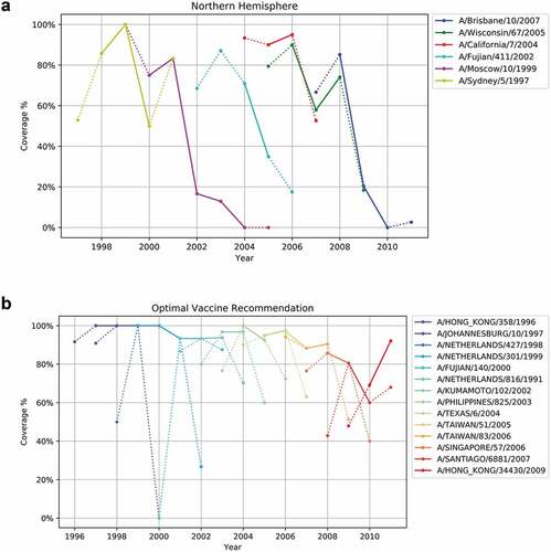
Figure 8(b) shows the “ideal” optimal vaccine recommendation based on the principle of maximizing the antigenicity coverage year by year. The optimal recommendation is obtained by solving the optimization problem retrospectively (This is the ideal case where it is assumed that knowledge of the circulating strains is known). The optimized result suggests a different virus strain for each year and presents a much better antigenicity coverage when compared to the WHO recommendation (Figure 8(a)). Specifically, the yearly coverage from 1997 to 2000 reaches up to 100% and above 90% from 2001 to 2008. In the optimized result, the model avoids recommending virus strains such as ‘A/Moscow/10/1999ʹ or ‘A/Brisbane/10/2007ʹ, for which coverage drops dramatically in 2002 and 2009, respectively. Instead, the optimized recommendation suggests ‘A/Netherlands/301/1999ʹ, ‘A/Fujian/140/2000ʹ, ‘A/Netherlands/816/1991ʹ, ‘A/Kumamoto/102/2002ʹ, ‘A/Philippines/825/2003ʹ, as replacement for ‘A/Moscow/10/1999ʹ and ‘A/Singapore/57/2006ʹ, ‘A/Santiago/6881/2007ʹ for ‘A/Brisbane/10/2007ʹ. However, an obvious decline in coverage from 2009 to 2010 suggests tremendous variety in the virus genotype. Therefore, both WHO’s suggestion and optimal recommendation exhibit coverage decrease. The average and median coverage of the optimized result are 92.80% and 95.89% with a standard deviation of 0.088, while the WHO’s recommendation has an average and median coverage of 59.43% and 74.07% with a standard deviation of 0.335.

Figure 9(a) shows the recommendation of vaccine composition produced by our CNN model using MDS. It results in an average coverage of 90.19% and standard deviation of 0.123. The CNN model produced the same vaccine recommendation as the optimal scenario for the period 1997 to 2000. The overall recommendation is different from the optimal scenario, and achieves slightly lower mean coverage, which is expected due to intrinsic predictive errors. Three strains (A/Texas/6/2004, A/Taiwan/83/2006, A/Hong Kong/34430/2009) reported by our CNN models present an upward trend in antigenicity coverage, indicating an increased vaccine efficacy during its installment. For 2009 to 2010, the CNN model suggests A/Switzerland/1397477/2008, which covers around 40% to 80% and achieves better performance than the WHO’s A/Brisbane/10/2007 recommendation. Contrasting Figures 8(a) and 9(a), we note that WHO often selects virus strains with small variation from year to year, and learns slowly and recovers once coverage dips very low; whereas our system-approach CNN model selects strains that can differ quite drastically from year to year. This rapid learning appears to offer consistently good coverage.

Figure 9. (a) Antigenicity coverage of vaccine recommendation by our CNN model. (b) Antigenicity coverage of vaccine recommendation by YC Liao’s model. (c) Antigenicity coverage of vaccine recommendation by J Qiu’s model. (d) Antigenicity coverage of vaccine recommendation by Y Yao’s model

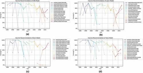
The average coverage of our CNN model outperforms all three models (Figure 9(a–d)). Table 10 summarizes and compares the coverage of vaccine recommendation from each model.

Table 10. Summary of model coverage

Model	Mean coverage (%)	Median coverage (%)	Standard deviation
Optimized recommendation	92.80	95.89	0.088
WHO recommendation	59.43	74.07	0.335
Liao’s	82.19	81.32	0.127
Qiu’s	82.10	92.98	0.258
Yao’s	85.28	93.33	0.194
Our CNN model	90.19	97.19	0.123

Discussion

Because of the continuous evolution of influenza viruses, vaccine recommendation remains a public health challenge. Due to the limitation of traditional HAI assay, in silico prediction of antigenicity is cost-effective and has become more widely accepted. Although many predictive models have been developed, this work represents the first time that CNNs are applied in this realm. Compared to other predictive models, our CNN model outperformed all others in terms of accuracy, sensitivity and specificity. To validate the usefulness of antigenic cartography, we constructed augmented models using cartography (multidimensional scaling) and evaluated their performance. Our results show that the CNN model trained with antigenic cartography can achieve better performance.

AAindex⁵⁶ is an excellent source for quantifying the property of protein sequences but has not been utilized comprehensively. Previous research primarily focused on limited properties of amino acids,^19,76 such as polarity and hydrophobicity. Y Yao¹¹ performed a comprehensive analysis of AAindex 2 using random forest. In this study, we systematically analyzed the predictability of all three AAindex datasets and optimized their selection using a CNN model. Prior studies of antigenicity prediction tended to select amino acid properties primarily from AAindex 1,^19,76 such as hydrophobicity, and polarity. However, our regression model showed that AAindex 1 has relatively low predictability compared to AAindex 2 and 3. The best blind validation MCC achieved by AAindex 1 is merely around 0. Combining AAindex 1 with AAindex 2 and 3 also reveals worse than mediocre predictive performance. Our findings suggest that it is reasonable to focus on AAindex 2 and 3 for antigenicity prediction.

We developed a pipeline for optimizing the selection of AAindex within a deep learning environment. Specifically, we adopted a non-gradient-based optimization approach – PSO – and used a small but carefully designed neural network to produce a good objective function value (that corresponds to a set of good combinations of AAindex). Multiple random starts of the optimization pipeline produced the best AAindex combinations with roughly half of the candidates from AAindex 2 and half from AAindex 3. The optimized combinations of AAindex elements prove to be not just a collection of individual elements with top performance in singular blind validation. Rather, there is a combinatorial effect from several “weak” AAindex elements, which is captured in the CNN model. In previous work,¹¹ Yao et al. proposed a stepwise method to select the AAindex elements, which initializes a pool of candidates by adding the best performing element sequentially. In contrast, our method starts with randomly selected elements multiple times, and thus avoids solutions potentially trapped in local optima. The PSO heuristic is stochastic in nature, so it is not guaranteed to produce the exact same result in repeated runs. However, the order of AAindex elements is guaranteed in our code if the same set of indices are returned as the optimizers. The mechanism ensures that the CNN will generate the same set of rules given the same set of AAindex elements.

The optimization of deep learning neural networks has been a major challenge for researchers, since it requires extensive empirical experiments. Although experience can help in tuning the parameters of a neural network, optimizing neural networks based on experience poses serious limits. Our proposed computational pipeline uses PSO to choose the best performing CNN architecture/structure, allowing flexibility in designing and testing different optimizers and tailoring algorithms to specific applications. Similarly, several random initializations were conducted when optimizing the selection of AAindex candidates. These ensure a diverse pool in generating the best performing CNN model.

A major benefit of the in-silico prediction of antigenicity is its application to vaccine recommendation and disease prevention. Vaccine recommendation remains a key challenge in combating seasonal influenza viruses and numerous predictive models have been investigated. In the 14 years 1998–2011 of antigenicity prediction (Table 8), our models achieved better MCC in blind validation testing when compared to the most promising published approaches. The accurate prediction can potentially facilitate better vaccine candidate selection and recommendation.

We also note the limitation on the analysis for the test set in the year 2000, where the specificity was merely 0.506, indicating the difficulty in predicting this particular dataset. Historical archives have shown that the flu season of 2000–2001 was especially mild and it was the first time since 1995 that H3N2 did not predominate.⁷⁷ The reason for a mild pandemic could be the lack of diverse variants, thus introducing difficulty in identifying distant mutants. Our model presents superior advantage even in such an extreme case where it still outperforms all other models.

We only performed year by year prediction up to 2011, since the T Bedford⁴⁹ data only cover up to 2011. Currently, we have collected only limited public data from WHO reports that cover beyond 2011. WHO and CDC do not publish all their antigenicity data in public reports. The quantity and quality of data are critical for superior prediction in deep learning. To fully explore the capacity of our CNN model, we need to seek close collaboration with WHO and CDC domain experts regarding better data access.

Contrasting to other approaches (Figures 8(a,b), 9(a–d) and 10), our CNN vaccine recommendation offers good coverage during the period of being a recommended strain. It tends to suggest a different virus strain more frequently than the WHO recommendation and presents a much better antigenicity coverage. The analysis supports that our model learns rapidly and selects strains based on global knowledge, whereas human experts take longer time (and lower coverage) to guide them to a new strain.

Unlike other approaches where a single mutation of amino acids is identified, our CNN model embeds their combinatorial relationship within a weighted matrix. One way to elucidate these relationships is to apply permutation to a specific position of the protein sequence across all samples and measure the change of performance.

Computationally, it takes approximately 30 min to an hour to train a CNN. But once trained, prediction is instant (merely seconds). This time expense estimate applies to all recommendations.

In summary, we demonstrated an innovative design and application of CNNs in the realm of Influenza antigenicity prediction. We proposed and validated the pipeline of amino acids selection, AAindex selection, and structural optimization of neural networks for Influenza vaccine recommendation. Our systems approach learns rapidly and advances the development of vaccine with higher accuracy. The beneficial effects include both saving of time and expenses.

Disclosure of potential conflicts of interest

No potential conflicts of interest were disclosed.

Additional information

Funding

The work is partially supported by a grant from by the U.S. National Institutes of Health (U19 AI090023), the U.S. Department of Health and Human Services and the Centers for Disease Control and Prevention. Findings and conclusions in this paper are those of the authors and do not necessarily reflect the views of the National Institutes of Health, U.S. Department of Health and Human Services and the Centers for Disease Control and Prevention.

Appendix

Figure A1. Shows an example of a simplified convolutional neural network

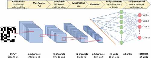
In this example, a CNN is designed to analyze a gray-scale input of 28x28x1 pixels. The first layer of CNN is always a convolution layer. Here, the first convolution employs a kernel of size 5 and scans the input using a step size of 1 to create a 24x24x1 panel. Multiple kernels are used each of which focuses on a specific characteristic of the input, such as edges, corners, diagonal lines, etc. This results in n1 convolved features. Next max-pooling of 2 × 2 is used to reduce the dimension from 24 to 12. The reduced convolved features are then fed into another convolution layer, using a kernel size of 5. The resulting convolved feature layers are of size 8x8, creating n2 convolved features. Next, max-pooling of 2 × 2 is used, resulting in the 4 × 4 panels. Finally flattening is performed to convert the matrices into a vector. This vector is then fully connected to the neural network (green) layer via an activation function. That is, each entry of the vector is connected to each node in this green layer. A dropout is used to fully connect this neural network to an output (red) class with reduced dimension. CNNs takes advantage of the hierarchical pattern in data and assembles more complex patterns using smaller and simpler patterns.

Users can choose different kernel sizes, calculation functions, different orders of applying the modular functions, and whether the CNN is fully connected or partially connected. These hyperparameters and the structure of the CNN can be optimized to arrive at a CNN design that is most “optimal” for the application at hand.

Table

Input	An image input is seen as an array of pixel values on a computer. Image Dimensions = Height x Breadth x Number of color channels. Each of these numbers is given a value from 0 to 255 which describes the pixel intensity at that point. These numbers are the inputs to the computer. The CNN will output numbers that describe the probability of the image being a certain class.
Convolutional layer	Convolutional layer first chooses a filter/kernel size. The model scans the input using the filter size. The scan moves from left to right with a certain step size until it parses the complete width of the input. It then traverses down the input with the same step size and repeats the process until the entire image is traversed. In this example, the 5 × 5 input matrix is scanned using a filter/kernel of size 3. This results in a 3 × 3 convolved feature output.
Padding	In Valid Padding, the convolved feature is reduced in dimensionality as compared to the input. In Same Padding, the dimensionality is either increased or remains the same. In this example, the input is padded with an extra layer of pixels on each side. This padded input is convolved via a kernel of size 3.
Pooling	The Pooling layer is responsible for reducing the spatial size of the Convolved Feature. This is to decrease the computational power required to process the data through dimensionality reduction. Max Pooling returns the maximum value from the portion of the image covered by the pool kernel. On the other hand, Average Pooling returns the average of all the values from the portion of the image covered by the pooling kernel. In general, max pooling performs better than average pooling. This example shows a 2 × 2 pooling on the input data via the two methods.
Flattening	Flattening converts a n x n matrix representation into a n^2 x 1 vector. This example represents the 3 × 3 matrix as a 9 × 1 vector.
Fully-Connected Neural Network	Fully connected means that every node in one layer has an edge that connects to every node in another layer. This example shows a fully connected with a dropout rate of 60%. It maps 25 green nodes to 10 red nodes. There is an edge between each pair of green-red nodes. In the output, each green node will be classified into exactly one of the 10 classes,

References

- WHO. Influenza (Seasonal). Geneva: World Health Organization; 2016.
- Blackburne BP, Hay AJ, Goldstein RA. Changing selective pressure during antigenic changes in human influenza H3. PLoS Pathog. 2008;4(5):e1000058. doi:10.1371/journal.ppat.1000058.
- Chan C-M, Chu H, Zhang AJ, Leung L-H, Sze K-H, Kao RYT, Chik KKH, To KKW, Chan JFW, Chen H, et al. Hemagglutinin of influenza A virus binds specifically to cell surface nucleolin and plays a role in virus internalization. Virology. 2016;494:78–88. doi:10.1016/j.virol.2016.04.008.
- Kageyama T, Fujisaki S, Takashita E, Xu H, Yamada S, Uchida Y, Neumann G, Saito T, Kawaoka Y, Tashiro M. Genetic analysis of novel avian A (H7N9) influenza viruses isolated from patients in China, February to April 2013. Euro Surveill. 2013;18(15):7–21.
- Holmes EC, Ghedin E, Miller N, Taylor J, Bao Y, St George K, Grenfell BT, Salzberg SL, Fraser CM, Lipman DJ, et al. Whole-genome analysis of human influenza A virus reveals multiple persistent lineages and reassortment among recent H3N2 viruses. PLoS Biol. 2005;3(9):e300. doi:10.1371/journal.pbio.0030300.
- De A, Nandy A. An insight to segment based genetic exchange in Influenza A virus: an in silico study. Basel (Switzerland); 2015. doi:10.3390/MOL2NET-1-b015.
- Peng D, Hu S, Hua Y, Xiao Y, Li Z, Wang X, Bi D. Comparison of a new gold-immunochromatographic assay for the detection of antibodies against avian influenza virus with hemagglutination inhibition and agar gel immunodiffusion assays. Vet Immunol Immunopathol. 2007;117(1):17–25. doi:10.1016/j.vetimm.2007.01.022.
- Stephenson I, Wood J, Nicholson K, Zambon M. Sialic acid receptor specificity on erythrocytes affects detection of antibody to avian influenza haemagglutinin. J Med Virol. 2003;70(3):391–98. doi:10.1002/()1096-9071.
- Sun H, Yang J, Zhang T, Long L-P, Jia K, Yang G, Webby RJ, Wan X-F. Using sequence data to infer the antigenicity of influenza virus. MBio. 2013;4(4):e00230–00213. doi:10.1128/mBio.00230-13.
- Ren X, Li Y, Liu X, Shen X, Gao W, Li J. Computational identification of antigenicity-associated sites in the hemagglutinin protein of a/h1n1 seasonal influenza virus. PLoS One. 2015;10(5):e0126742. doi:10.1371/journal.pone.0126742.
- Yao Y, Li X, Liao B, Huang L, He P, Wang F, Yang J, Sun H, Zhao Y, Yang J. Predicting influenza antigenicity from Hemagglutinin sequence data based on a joint random forest method. Sci Rep. 2017;7. doi:10.1038/s41598-017-01699-z.
- Liao Y-C, Lee M-S, Ko C-Y, Hsiung CA. Bioinformatics models for predicting antigenic variants of influenza A/H3N2 virus. Bioinformatics. 2008;24(4):505–12. doi:10.1093/bioinformatics/btm638.
- Pan K, Subieta KC, Deem MW. A novel sequence-based antigenic distance measure for H1N1, with application to vaccine effectiveness and the selection of vaccine strains. Protein Eng Des Sel. 2011;24(3):291–99. doi:10.1093/protein/gzq105.
- Steinbrück L, Klingen T, McHardy A. Computational prediction of vaccine strains for human influenza A (H3N2) viruses. J Virol. 2014;88(20):12123–32. doi:10.1128/JVI.01861-14.
- Lees WD, Moss DS, Shepherd AJ. A computational analysis of the antigenic properties of haemagglutinin in influenza A H3N2. Bioinformatics. 2010;26(11):1403–08. doi:10.1093/bioinformatics/btq160.
- Lee M-S, Chen M-C, Liao Y-C, Hsiung CA. Identifying potential immunodominant positions and predicting antigenic variants of influenza A/H3N2 viruses. Vaccine. 2007;25(48):8133–39. doi:10.1016/j.vaccine.2007.09.039.
- Neher RA, Bedford T, Daniels RS, Russell CA, Shraiman BI. Prediction, dynamics, and visualization of antigenic phenotypes of seasonal influenza viruses. Proc Natl Acad Sci. 2016;113(12):E1701–E1709. doi:10.1073/pnas.1525578113.
- Veljkovic V, Paessler S, Glisic S, Prljic J, Perovic VR, Veljkovic N, Scotch M. Evolution of 2014/15 H3N2 Influenza viruses circulating in US: consequences for vaccine effectiveness and possible new pandemic. Front Microbiol. 2015;6. doi:10.3389/fmicb.2015.01456.
- Qiu J, Qiu T, Yang Y, Wu D, Cao Z. Incorporating structure context of HA protein to improve antigenicity calculation for influenza virus A/H3N2. Sci Rep. 2016;6:31156.
- WHO. A description of the process of seasonal and H5N1 Influenza vaccine virus selection and development. World Health Organization; 2007.
- Krizhevsky A, Sutskever I, Hinton GE. Imagenet classification with deep convolutional neural networks. Adv Neural Inf Process Syst. 2012;1:1097–105.
- Simard PY, Steinkraus D, Platt JC. Best practices for convolutional neural networks applied to visual document analysis. ICDAR. Seventh International Conference on Document Analysis and Recognition, 2003. Proceedings.2003;958–62. https://www.semanticscholar.org/paper/Best-practices-for-convolutional-neural-networks-to-Simard-Steinkraus/5562a56da3a96dae82add7de705e2bd841eb00fc
- Toderici KG, Shetty S, Leung T, Sukthankar R, Fei-Fei L. Large-scale video classification with convolutional neural networks. Proceedings of the IEEE conference on Computer Vision and Pattern Recognition; Columbus, OH; 2014. p. 1725–32. doi:10.1109/CVPR.2014.223.
- Ji S, Xu W, Yang M, Yu K. 3D convolutional neural networks for human action recognition. IEEE Trans Pattern Anal Mach Intell. 2013;35(1):221–31. doi:10.1109/TPAMI.2012.59.
- Kim Y. Convolutional neural networks for sentence classification. arXiv Preprint arXiv:1408.5882. 2014.
- Abdel-Hamid O, A-r M, Jiang H, Penn G. Applying convolutional neural networks concepts to hybrid NN-HMM model for speech recognition. Acoustics, Speech and Signal Processing (ICASSP), 2012 IEEE International Conference on, (IEEE); New York (NY); 2012. p. 4277–80.
- Wang T, Wu DJ, Coates A, Ng AY. End-to-end text recognition with convolutional neural networks. Pattern Recognition (ICPR), 2012 21st International Conference on, (IEEE); Tsukuba (Japan); 2012. p. 3304–08.
- Cireşan DC, Giusti A, Gambardella LM, Schmidhuber J. Mitosis detection in breast cancer histology images with deep neural networks. International Conference on Medical Image Computing and Computer-assisted Intervention, Springer; Nagoya (Japan); 2013. p. 411–18.
- Wang H, Cruz-Roa A, Basavanhally A, Gilmore H, Shih N, Feldman M, Tomaszewski J, Gonzalez F, Madabhushi A. Mitosis detection in breast cancer pathology images by combining handcrafted and convolutional neural network features. J Med Imaging. 2014;1(3):034003–034003. doi:10.1117/1.JMI.1.3.034003.
- Cruz-Roa A, Basavanhally A, González F, Gilmore H, Feldman M, Ganesan S, Shih N, Tomaszewski J, Madabhushi A. Automatic detection of invasive ductal carcinoma in whole slide images with convolutional neural networks. SPIE medical imaging, (International Society for Optics and Photonics); San Diego (CA); 2014. p. 904103–904103.
- QiD, Chen H, Yu L, Zhao L, Qin J, Wang D, Ct Mok V, Shi L, Heng PA. Automatic detection of cerebral microbleeds from MR images via 3D convolutional neural networks. IEEE Trans Med Imaging. 2016;35(5):1182–95. doi:10.1109/TMI.2016.2528129.
- Ghafoorian M, Karssemeijer N, Heskes T, van Uden IWM, de Leeuw FE, Marchiori E, van Ginneken B, Platel B. Non-uniform patch sampling with deep convolutional neural networks for white matter hyperintensity segmentation. Biomedical Imaging (ISBI), 2016 IEEE 13th International Symposium on, (IEEE); Prague (Czech Republic); 2016. p. 1414–17.
- Sarraf S, Tofighi G. Classification of alzheimer’s disease using fMRI data and deep learning convolutional neural networks. arXiv Preprint arXiv:1603.08631. 2016.
- Quang D, Xie X. DanQ: a hybrid convolutional and recurrent deep neural network for quantifying the function of DNA sequences. Nucleic Acids Res. 2016;44(11):e107–e107. doi:10.1093/nar/gkw226.
- Kim J. Detecting influenza outbreaks in United States by analyzing climatic heat maps using convolutional neural network. Internationa Conference Data Mining| DMIN'17, SBN: 1-60132-453-7; CSREA Press; Las Vegas (NV); 2017. p. 24–27.
- Zhong S, Bian L. Predicting Influenza dynamics using a deep learning approach. Int Conf GISci Short Pap Proc. 2016;1. doi:10.21433/B3113969C18V.
- Garro BA, Vázquez RA. Designing artificial neural networks using particle swarm optimization algorithms. Comput Intell Neurosci. 2015;2015:61. doi:10.1155/2015/369298.
- Zoph B, Le QV. Neural architecture search with reinforcement learning. arXiv Preprint arXiv:1611.01578. 2016.
- Albelwi S, Mahmood A. A framework for designing the architectures of deep convolutional neural networks. Entropy. 2017;19:242.
- Bergstra JS, Bardenet R, Bengio Y, Kégl B. Algorithms for hyper-parameter optimization. Adv Neural Inf Process Syst. 2011;24:2546–54.
- Karaboga D, Akay B, Ozturk C. Artificial bee colony (ABC) optimization algorithm for training feed-forward neural networks. MDAI. 2007;7:318–19.
- Bergstra J, Bengio Y. Random search for hyper-parameter optimization. J Mach Learn Res. 2012;13:281–305.
- Snoek J, Larochelle H, Adams RP. Practical bayesian optimization of machine learning algorithms. Adv Neural Inf Process Syst. 2012;25:2951–59.
- Saxena S, Verbeek J. Convolutional neural fabrics. Adv Neural Inf Process Syst. 2016;29:4053–61.
- Mendoza H, Klein A, Feurer M, Springenberg JT, Hutter F. Towards automatically-tuned neural networks. Workshop Autom Mach Learn. 2016;64:58–65.
- Yao X. Evolving artificial neural networks. Proc IEEE. 1999;87(9):1423–47. doi:10.1109/5.784219.
- Yu J, Xi L, Wang S. An improved particle swarm optimization for evolving feedforward artificial neural networks. Neural Process Lett. 2007;26(3):217–31. doi:10.1007/s11063-007-9053-x.
- Young SR, Rose DC, Karnowski TP, Lim S-H, Patton RM. Optimizing deep learning hyper-parameters through an evolutionary algorithm. Proceedings of the Workshop on Machine Learning in High-Performance Computing Environments, ACM; Austin (TX); 2015. p 4.
- Bedford T, Suchard MA, Lemey P, Dudas G, Gregory V, Hay AJ, McCauley JW, Russell CA, Smith DJ, Rambaut A. Integrating influenza antigenic dynamics with molecular evolution. Elife. 2014;3:e01914. doi:10.7554/eLife.01914.
- Smith DJ, Lapedes AS, de Jong JC, Bestebroer TM, Rimmelzwaan GF, Osterhaus ADME, Fouchier RAM. Mapping the antigenic and genetic evolution of influenza virus. Science. 2004;305(5682):371–76. doi:10.1126/science.1097211.
- Bao Y, Bolotov P, Dernovoy D, Kiryutin B, Zaslavsky L, Tatusova T, Ostell J, Lipman D. The influenza virus resource at the national center for biotechnology information. J Virol. 2008;82(2):596–601. doi:10.1128/JVI.02005-07.
- Zhang Y, Aevermann BD, Anderson TK, Burke DF, Dauphin G, Gu Z, He S, Kumar S, Larsen CN, Lee AJ. Influenza research database: an integrated bioinformatics resource for influenza virus research. Nucleic Acids Res. 2016;45(D1):D466–D474. doi:10.1093/nar/gkw857.
- Elbe S, Buckland-Merrett G. Data, disease and diplomacy: GISAID’s innovative contribution to global health. Global Challenges. 2017;1(1):33–46. doi:10.1002/gch2.1018.
- Edgar RC. MUSCLE: multiple sequence alignment with high accuracy and high throughput. Nucleic Acids Res. 2004;32(5):1792–97. doi:10.1093/nar/gkh340.
- Ashkenazy H, Erez E, Martz E, Pupko T, Ben-Tal N. ConSurf 2010: calculating evolutionary conservation in sequence and structure of proteins and nucleic acids. Nucleic Acids Res. 2010;38(suppl_2):W529–W533. doi:10.1093/nar/gkq399.
- Kawashima S, Pokarowski P, Pokarowska M, Kolinski A, Katayama T, Kanehisa M. AAindex: amino acid index database, progress report 2008. Nucleic Acids Res. 2007;36(suppl_1):D202–D205. doi:10.1093/nar/gkm998.
- Chollet F. Keras. GitHub; 2015Chollet, F. (2015) keras, GitHub. https://github.com/fchollet/keras.
- Lee EK, Nakaya HI, Yuan F, Querec TD, Burel G, Pietz FH, Benecke BA, Pulendran B. Machine learning for predicting vaccine immunogenicity. Interfaces. 2016;46(5):368–90. doi:10.1287/inte.2016.0862.
- Querec TD, Akondy RS, Lee EK, Cao W, Nakaya HI, Teuwen D, Pirani A, Gernert K, Deng J, Marzolf B, et al. Systems biology approach predicts immunogenicity of the yellow fever vaccine in humans. Nat Immunol. 2009;10(1):116. doi:10.1038/ni.1688.
- Kennedy J, Mendes R. Neighborhood topologies in fully informed and best-of-neighborhood particle swarms. IEEE Trans Syst Man Cybern C Appl Rev. 2006;36(4):515–19. doi:10.1109/TSMCC.2006.875410.
- Kennedy J. Particle swarm optimization. Encyclopedia of machine learning, Springer; 2011. p. 760–66. doi:10.1177/1753193411423140.
- Dennis J, Woods DJ. Optimization on microcomputers: the Nelder-Mead simplex algorithm. New Comput environ. 1987;11:116–22.
- Powell MJ. An efficient method for finding the minimum of a function of several variables without calculating derivatives. Comput J. 1964;7(2):155–62. doi:10.1093/comjnl/7.2.155.
- Straeter TA. On the extension of the Davidson-Broyden class of rank one, quasi-newton minimization methods to an infinite dimensional hilbert space with applications to optimal control problems; NASA Technical Report Server, NASA; USA; 1971.
- Fletcher R. Practical methods of optimization. John Wiley & Sons; 2013. Wiley Online.
- Byrd RH, Lu P, Nocedal J, Zhu C. A limited memory algorithm for bound constrained optimization. SIAM J Sci Comput. 1995;16(5):1190–208. doi:10.1137/0916069.
- Martens J. Deep learning via Hessian-free optimization. ICML. Proceedings of the 27th International Conference on Machine Learning; Haifa, Israel; 2010. p. 735–42.
- Conn AR, Scheinberg K, Toint PL. On the convergence of derivative-free methods for unconstrained optimization. In: Iserles A, Buhmann M, editors. Approximation theory and optimization: Tributes to M. J. D. Powell. Cambridge (UK): Cambridge University Press; 1997, p. 83–108.
- Nocedal J, Wright SJ. Sequential quadratic programming. Switzerland: Springer; 2006.
- Georgiev AG. Interpretable numerical descriptors of amino acid space. J Comput Biol. 2009;16(5):703–23. doi:10.1089/cmb.2008.0173.
- van Westen GJ, Swier RF, Cortes-Ciriano I, Wegner JK, Overington JP, IJzerman AP, van Vlijmen HW, Bender A. Benchmarking of protein descriptor sets in proteochemometric modeling (part 2): modeling performance of 13 amino acid descriptor sets. J Cheminform. 2013;5(1):42. doi:10.1186/1758-2946-5-42.
- Control CfD & Prevention. Preliminary assessment of the effectiveness of the 2003-04 inactivated influenza vaccine–Colorado, December 2003. MMWR Morb Mortal Wkly Rep. 2004;53(1):8.
- Belongia EA, Kieke B, Donahue J, Greenlee R, Balish A, Foust A, Lindstrom S, Shay D. Effectiveness of inactivated influenza vaccines varied substantially with antigenic match from the 2004–2005 season to the 2006–2007 season. J Infect Dis. 2009;199(2):159–67. doi:10.1086/597213.
- Saito R, Suzuki H, Oshitani H, Sakai T, Seki N, Tanabe N. The effectiveness of influenza vaccine against influenza A (H3N2) virus infections in nursing homes in Niigata, Japan, during the 1998-1999 and 1999-2000 seasons. Infect Control Hosp Epidemiol. 2002;23(2):82–86. doi:10.1086/502011.
- Control CfD & Prevention. Interim within-season estimate of the effectiveness of trivalent inactivated influenza vaccine–Marshfield, Wisconsin, 2007-08 influenza season. MMWR Morb Mortal Wkly Rep. 2008;57(15):393.
- Lee M-S, Chen JS-E. Predicting antigenic variants of influenza A/H3N2 viruses. Emerg Infect Dis. 2004;10(8):1385. doi:10.3201/eid1008.040107.
- CDC. 2000-2001 Influenza season summary. Atlanta (GA): Centers for Disease Control and Prevention; 2001.