Yule's lambdagram revisited and reclaimed

Abstract

In this article, the lambdagram, proposed by Yule in his last time series paper published in 1945, is revisited using modern theoretical and computational developments unavailable to him. Although it is not particularly good at identifying stationary processes, the lambdagram is found to be much more useful for distinguishing between trend and difference stationary processes. The lambdagram is applied to the Nelson–Plosser data and the conclusions drawn from using it are compared with other analyses of this data set.

I. Introduction

During the 1920s, Yule published three papers (1921, 1926, 1927) that were instrumental in laying down many of the foundations of modern time series analysis.¹ After a hiatus of almost 20 years, Yule's (1945) last foray into the subject – when he was well into his seventies – was a paper published in the Journal of the Royal Statistical Society in 1945 where he studied the ‘internal correlations’ of a time series by way of a statistic, which he termed the coefficient of linkage, and a related graphical display, which he called the lambdagram. Apart from the note published by Kendall (1945a) as an addendum to the paper and the calculation of a lambdagram for the sunspot index in Ghurye (1950), almost no other references to this concept can be found until it was ‘rediscovered’ by Mills (2011, §8.8–8.9).² The purposes of the present article are to revisit Yule's lambdagram from a modern perspective and to assess its usefulness as an essentially graphical device for distinguishing between difference and trend stationary processes by using both theoretical and computational developments that were unavailable to Yule and Kendall at their time of writing. In doing so, we hope to reclaim the lambdagram as a fitting tribute to one of Britain's most prestigious statisticians.

II. Yule's Lambdagram

In a sequence of papers published during the war on the behaviour of agricultural time series, Kendall (1941, 1943, 1944, 1945b) focused his attention on oscillatory processes, that is, those that could be characterized by second-order autoregressions having complex roots, examining in detail the behaviour of the serial correlations from such processes. Yule (1945) decided to break away from the analysis of oscillatory processes to consider an alternative way of characterizing the properties of a time series. This approach was based on a result reported in Yule and Kendall (1950, p. 390) concerning the variance of the means of independent samples of size n drawn from a longer time series (say of length T) and focused on the behaviour of the quantity as n increases. As Yule showed, this can be written as where so that it is the second sum of the serial correlations scaled by the factor 2/n. If S_m has a finite value such that m and T_m become negligible when compared with n and T_n, then the limiting value of λ_n is 2S_m.

Yule termed λ_n the coefficient of linkage. If λ_n=0, then either all of the serial correlations are zero or any positive correlations are balanced by negative ones. Yule showed that , and the implications of these limits are revealed when we use Yule and Kendall's result that the variance of the means of independent samples of length n is , where σ² is the variance of the series itself. The maximum value occurs when ρ_i=1 for , so that the terms of samples of size n are completely linked together and the means of the successive samples have the same variance as the series itself. The minimum value is achieved when the terms in the sample are as completely negatively linked as possible (bearing in mind that not all pairs in a sample can have a correlation of −1) and the means of the successive samples have zero variance and hence do not vary at all. If λ_n=0, then the terms are unlinked and the means of the successive samples behave like the means of random samples. Yule termed a plot of λ_n against n a lambdagram, although for ease of exposition we shall also refer to λ_n itself by this term.

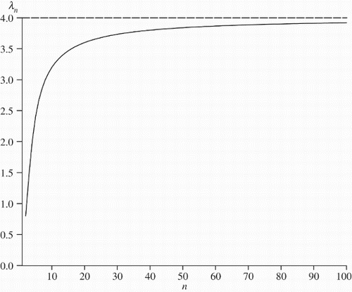
If a correlated series is formed by summing a random series in overlapping runs of k terms, that is, as , then , , ρ_i=0, i≥k, and, in the limit, . Thus, all values of λ_n are positive and the lambdagram clearly approaches a limit, as can be seen in Fig. 1, which displays the lambdagram for k=5.

Figure 1. Lambdagram for a correlated series formed by summing the terms of a random series in overlapping groups of 5

The lambdagram is, in fact, related to the expected ‘intensity’ of a stationary zero mean time series, defined subsequent to Yule by Bartlett (1950, Equation 19) as in which p and ω are the particular period and frequency linked by . For ω=0, so that : that is, the lambdagram is a linear transformation of the frequency zero spectral density, where 2σ² is the expected intensity of a completely random series.

III. Yule's Empirical Lambdagrams

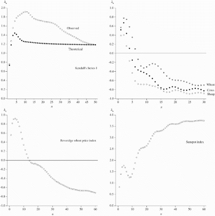
Figure 2 displays calculated lambdagrams (i.e. those obtained by replacing the ρ_i by the sample serial correlations for a variety of series analysed by Yule and Kendall, as well as the sunspot index observed for the period 1700–2007 (n is generally set at the value chosen by Yule). They display a variety of patterns, with Kendall's agricultural series having similar lambdagrams both between themselves and with Beveridge's (1921) detrended wheat price index (the ‘Index of Fluctuation’). The sunspot index has a lambdagram that is generally increasing towards a maximum that appears to be in the region of 3.75, while the lambdagram of Kendall's Series I (given in Kendall, 1945b, Table 2) seems to be declining towards a value of around 1.2.

Figure 2. Calculated lambdagrams for a variety of time series

Since the latter series is known to be generated by the oscillatory process with a=1.1 and b=−0.5 and with being independently drawn from a rectangular distribution, Kendall (1945a) analysed the implications for the lambdagram of this generating process, showing that the limiting value of the lambdagram of Equation 3 for large n is a result that could subsequently be obtained using the relationship in Equation 2.

If b=−1, then it is easy to see that λ=−1, while using standard results linking the autoregressive parameters to the first two serial correlations, that is, allows λ to be written as For an oscillatory process, because b<0 and . Hence, λ will be positive or negative depending on whether ρ₁ is greater than or less than | b |.

Of course, the ‘true’ serial correlations are given by ρ₀=1 and , followed by the recursion . The set of theoretical serial correlations thus generated with a=1.1 and b=−0.5 can then be used to calculate the ‘theoretical’ lambdagram, which is shown with the empirical lambdagram of Series I in Fig. 2. The limiting value from Equation 4 is , and by n=50, both the empirical and theoretical lambdagrams are consistent with this and are themselves almost identical. However, as Kendall (1945a, p. 228) remarked,

throughout the previous course of the lambdagram the observed values are much higher than the theoretical values.

It seems clear that these differences are due to the failure of the observed correlations to damp out according to theoretical explanation. If this is the correct explanation I should expect it to be equally possible on occasion for the observations to be systematically lower than the theoretical over parts of the range. Series I, it is to be remembered, is based on 480 terms and we are entitled to expect that for shorter series observation and theory will be less in agreement.

Values for a and b for each of the other series shown in Fig. 2 can be computed using Equation 5 and the limiting values of the lambdagram calculated using Equation 4. This produces λ values of −0.421, −0.394 and 0.004 for the sheep, wheat and cow series, respectively, 0.876 for the Beveridge wheat price index and 0.935 for the sunspot index. From Fig. 2, it is clear that none of these limiting values seem to be very close to the values that the empirical lambdagrams appear to be tending towards. While Kendall thought that short oscillatory series would give rise to serial correlations that did not damp out according to theoretical expectation, and hence empirical lambdagrams at odds with their theoretical counterparts, an alternative explanation for the observed disparity could also be that these series are not adequately represented by oscillatory processes, so that more general autoregressions are required.³

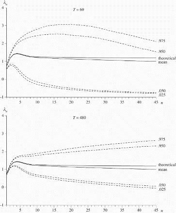
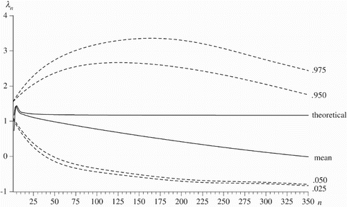
Notwithstanding this possibility, what sort of variation should be expected from computing a lambdagram from process 3? Figure 3 shows the mean and theoretical lambdagrams, along with 2.5%, 5%, 95% and 97.5% percentiles, from 10,000 simulations of process 3 with a=1.1, b=−0.5 and for T=480 observations, the length of the series generated by Kendall. Values for n≤350 are shown, and throughout this interval, the mean lambdagram is consistently smaller than its theoretical value and is declining in size as n increases, with the percentiles showing that the empirical lambdagram is distributed across a wide range of values.

Figure 3. Mean and theoretical lambdagrams, along with 2.5%, 5%, 95% and 97.5% percentiles from 10,000 simulations of process 3 with a=1.1, b=−0.5 and ϵ_t∼ N(0, 1) for T=480 for n≤350

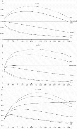
Figure 4 repeats the exercise for a smaller sample of size T=60 and shows the resulting lambdagrams and percentiles for n≤45, along with the analogous values from the longer sample, while Fig. 5 repeats Fig. 3 for the AR(1) process defined by setting, in turn, a=0, 0.5 and 0.95 (with b=0), for which the theoretical lambdagrams are such that λ_n=0, and , respectively. It is clear that the findings of Fig. 3 are replicated in general detail, in that the mean lambdagram is biased downwards from the theoretical lambdagram and that the empirical lambdagram covers a wide range of values. This suggests that, for stationary series, little confidence can be placed on the lambdagram for identifying the underlying process generating the data. However, closer examination of the a=0.95 case reveals that, for small n, the bounds are reasonably narrow, suggesting that the lambdagram may nevertheless be useful for identifying highly persistent processes.

Figure 4. Mean and theoretical lambdagrams, along with 2.5%, 5%, 95% and 97.5% percentiles from 10,000 simulations of process 3 with a=1.1, b=−0.5 and ϵ_t∼ N(0, 1) for T=60 and T=480 for n≤45

Figure 5. Mean and theoretical lambdagrams, along with 2.5%, 5%, 95% and 97.5% percentiles from 10,000 simulations of process 2 with a=0, 0.5 and 0.95, b=0 and ϵ_t∼ N(0, 1) for T=480 for n≤350

IV. The Lambdagram for a Unit Root Process

Although the lambdagram thus seems to be of only limited use for identifying stationary processes and, as such, might be regarded simply as a historical curiosity, its behaviour for persistent processes makes it natural, from a modern time series perspective unavailable to Yule and Kendall, to consider its behaviour for unit root processes. Clearly, for a random walk, all theoretical serial correlations tend to unity for large T so that, as indeed observed by Yule, , but what happens in finite samples when sample serial correlations are used? Since , it follows that the probability that given ρ₁=1 approaches 0.6826 (the probability that a χ²(1) variate is less than 1) as T gets large (Fuller, 1976, p. 370). The statistic has a known asymptotic distribution (Phillips, 1987) and finite sample critical values, obtained by simulation, that were originally tabulated by Fuller (1976, Table 8.5.1) and improved upon by MacKinnon (1996). On denoting this asymptotic distribution as , Hassler (1994) showed that when , under the set of assumptions used by Phillips (1987), the serial correlation r_i converges in distribution to a multiple of the distribution, namely that is, that Using this result, it then follows that Clearly, as T→∞, so r_i→1 and It is also clear that, for fixed declines almost linearly in i and at some value of i will fall below –1, so that this result is only useful for small i and hence small n.

Resorting to simulation for large values of n, Fig. 6 thus shows the simulated distribution of for n≤350 and T=480 from the random walk obtained by setting a=1 and b=0 in Equation 3. For this value of T, the statistic has 2.5% and 5% critical values of −16.74 and −13.97, implying that and (the simulated values of these critical values were 0.9645 and 0.9704). From Equation 6, , and , compared with the simulated values of 4.662, 15.962 and 21.552, respectively. After this, the two begin to diverge substantially with, for example, from Equation 6 compared with a simulated value of 32.48 (the value at which r_i becomes less than −1 using Equation 6 is n=60).

Figure 6. Mean and ‘theoretical’ lambdagrams, along with 2.5%, 5%, 95% and 97.5% percentiles from 10,000 simulations of the random-walk process obtained by setting a=1 and b=0 in Equation 2 with ϵ_t∼ N(0, 1) for T=480 for n≤350

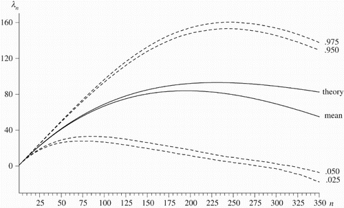
The ‘theoretical’ lambdagram shown in Fig. 6 is that obtained using the result of Wichern (1973), who derived the ratio of the expectation of the lag-i sample autocovariance, c_i, to the expectation of the sample variance, c₀, for a random walk as Although this ratio is clearly not E(r_i), it should provide some insight into the behaviour that could be expected from the lambdagram of a random walk. Some limited simulation evidence provided by Wichern suggests that this formula over-estimates the average value of r_i, and this is confirmed in Fig. 6, with this ‘theoretical’ lambdagram being larger than the mean lambdagram and the difference increasing with n.

Indeed, as n increases, the spread of the distribution increases, no doubt because of the imprecision with which higher order serial correlations are estimated. Nevertheless, for small n, the bounds remain quite precise, giving some hope that the lambdagram may be a useful discriminatory device for unit root processes.

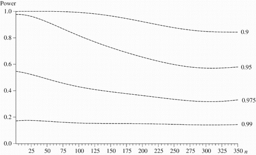
Figure 7 investigates the power, using 5% level tests, of the lambdagram for stationary alternatives to the driftless random walk for a=0.9, 0.95, 0.975 and 0.99. This confirms the conjecture made from Fig. 6: for n≤50, the power is reasonably good for a≤0.975, and suggests that the lambdagram might be a useful graphical device for helping to distinguish alternative forms of nonstationarity in the observed time series.

Figure 7. Power functions for a random walk against an AR(1) alternative with coefficients 0.9, 0.95, 0.975 and 0.99, respectively

V. Lambdagrams for the Nelson–Plosser Data Set

To investigate this possibility further, lambdagrams were calculated (for n≤50) for the 14 series analysed in Nelson and Plosser's (1982) seminal article on distinguishing between difference and trend stationary processes, which have since been used many times to illustrate new techniques and tests in time series econometrics, with a notable recent and relevant example being Andreou and Spanos (2003). Table 1 reports the estimates of the drift parameter c from fitting the model to each of the series, along with additional details. Since most of the series exhibit some form of drift, they were detrended by extracting a linear trend prior to the lambdagrams being calculated.

Table 1. Nelson–Plosser data set: t_c=0 denotes the t-ratio testing c=0

Series	Sample	T
Bond yields	1900–70	71	0.0614[1.71]
Consumer prices	1860–1970	111	0.0133[2.43]
Employment	1890–1970	81	0.0161[3.76]
Nominal GNP	1909–70	62	0.0553[4.40]
Industrial production	1860–1970	111	0.0434[4.50]
Money stock	1889–1970	82	0.0582[8.46]
Real per capita GNP	1909–70	62	0.0164[1.96]
GNP deflator	1889–1970	82	0.0204[3.52]
Real GNP	1909–70	62	0.0298[3.60]
Real wages	1900–70	71	0.0183[4.14]
Stock prices	1871–1970	100	0.0291[1.80]
Unemployment	1890–1970	81	0.0025[0.05]
Velocity	1869–1970	102	–0.012[1.71]
Wages	1900–70	71	0.0402[4.95]

Note: Logarithms were used for all series except for the bond yield.

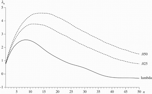
The lambdagram for unemployment, shown in Fig. 8, clearly identifies the series as being stationary, which is consistent with all other analyses of this variable. The series is, in fact, well fitted by the oscillatory process , having complex characteristic roots of and a limiting lambdagram value of λ=3.4, which the empirical lambdagram is still some way below by n=50, consistent with our earlier results.

Figure 8. Lambdagram for unemployment

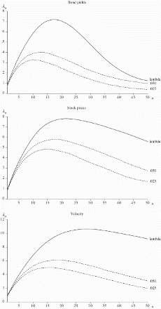
The lambdagrams for bond yields, stock prices and velocity are shown in Fig. 9. For all three series, there is some uncertainty as to whether they have significant drifts, but all are clearly seen to be nonstationary from their lambdagrams. Since it is difficult to argue that bond yields should have a drift in either direction over long periods of time, it appears sensible to conclude that they are difference stationary without a drift. Stock prices and velocity are clearly difference stationary irrespective of whether a drift is assumed or not.

Figure 9. Lambdagrams for bond yields, stock prices and velocity

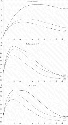
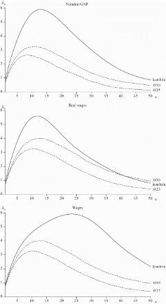
Figure 10 shows lambdagrams for consumer prices, real per capita Gross National Product (GNP) and real GNP, and all three series are found to be nonstationary. Given that all appear to have significant drifts, we thus conclude that all are difference stationary. The lambdagrams for nominal GNP and real and nominal wages are shown in Fig. 11 and demonstrate that all series are clearly difference stationary as well.

Figure 10. Lambdagrams for consumer prices, real per capita GNP and real GNP

Figure 11. Lambdagrams for nominal GNP and real and nominal wages

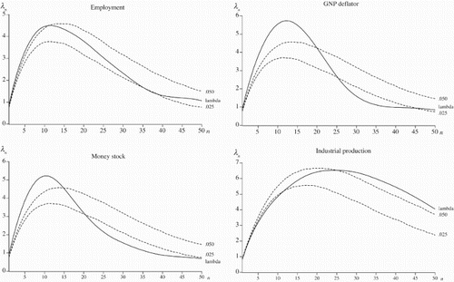
The lambdagrams for the remaining four series, employment, the money stock, the GNP deflator and industrial production, are shown in Fig. 12. Employment seems to be trend stationary, whereas there is some ambiguity concerning industrial production, money stock and the GNP deflator: if the behaviour of the lambdagram for lower values of n is considered to be the best indication of the form of nonstationarity, then industrial production is signalled to be trend stationary and money stock and the GNP deflator difference stationary.

Figure 12. Lambdagrams for industrial production, employment, money stock and the GNP deflator

It is interesting to compare these results with those originally obtained by Nelson and Plosser (1982) and subsequently refined by Perron (1989, 1997) and Andreou and Spanos (2003). Nelson and Plosser concluded that all variables, apart from the stationary unemployment series, were difference stationary. Perron (1989) included a break at 1929 and found that only three series, bond yields, consumer prices and velocity, continued to exhibit difference stationarity. Perron (1997) chose the break dates endogenously and, with certain other refinements concerning lag length selection, found that the GNP deflator was also difference stationary. Andreou and Spanos widened the model specification further and found that these four series remained difference stationary, although bond yields and stock prices exhibited other forms of (covariance) nonstationarity.

The purely ‘nonparametric’ lambdagrams reported here are consistent with the general finding that bond yields, stock prices and velocity are difference stationary and that unemployment is stationary. For the other series, they tend to be consistent with the original findings of Nelson and Plosser, and not with those from the more refined later analyses, which is hardly surprising given the simplicity of this graphical approach.

VI Conclusions

After its publication in 1945, Yule's lambdagram appears to have been quickly forgotten, presumably because it did not seem to be a very useful device for identifying the underlying models generating stationary time series. Nonstationary time series were simply unable to be considered at this stage in the development of time series analysis, with Beveridge (1921) detrending his wheat price series by dividing it by a 31-year moving average to obtain his Index of Fluctuation and Kendall detrending all his agricultural series by 9-year moving averages prior to analysing them as oscillatory processes (1941). The distinctive features of the lambdagram only appear, however, for unit root processes, but this was simply beyond the theoretical and computational abilities of the time series community in the mid-1940s.

While it is delightful to be able to reclaim this idea from one of the seminal figures in the history of time series analysis, the lambdagram certainly cannot, or indeed should not, replace any of the now standard approaches to discriminating between different forms of stationary and nonstationary processes. However, with the statistical community recognizing more than ever the potential importance of graphical displays for providing evidence additional to that obtained from formal statistical modelling and testing, Yule's lambdagram may yet prove to be a useful auxiliary graphical device for discriminating between these different processes. Indeed, for someone who, according to Kendall (1952, p. 158), had ‘the legitimate scepticism of a practical statistician for the monstrous regiment of mathematicians’, this may well be a fitting tribute to such a great statistician.

Notes

¹A detailed examination of Yule's time series research is provided by Mills (2011, Chapters 5 and 6), while Aldrich (1995, 1998) discusses his work on correlation and regression and Tabery (2004) discusses his contribution to the ‘evolutionary synthesis’ in biology and the biometric–Mendelian debate. His textbook Introduction to the Theory of Statistics was very influential and ran to 14 editions during his lifetime, with the later editions co-authored with his close friend Maurice Kendall. For biographical details of Yule and a full list of his publications, see Kendall (1952) and also Williams (2004).

²A statistic related to the lambdagram has been used to analyse counts of events from point processes (see Lewis and Govier, 1964).

³This is certainly true for the sunspot index, where at least an AR(9) process is required to adequately model the series (see Morris, 1977; Mills, 2011, Chapter 9). Sargan (1953) actually fitted model 3 with a=0.73 and b=−0.31 to Beveridge's Index of Fluctuation, but Quenouille (1947), in the first application of a goodness-of-fit test for autoregressions, found that such a model was misspecified, although his test found no evidence against such a model for wheat prices.

References

- Aldrich, J. (1995) Correlations genuine and spurious in Pearson and Yule, Statistical Science, 10, 364–76.
- Aldrich, J. (1998) Doing least squares: perspectives from Gauss and Yule, International Statistical Review, 68, 155–72.
- Andreou, E. and Spanos, A. (2003) Statistical adequacy and the testing of trend versus difference stationarity, Econometric Reviews, 22, 217–37. doi: 10.1081/ETC-120023897
- Bartlett, M. S. (1950) Periodogram analysis and continuous spectra, Biometrika, 37, 1–16.
- Beveridge, W. H. (1921) Weather and harvest cycles, Economic Journal, 31, 429–52. doi: 10.2307/2223074
- Fuller, W. A. (1976) Introduction to Statistical Time Series, Wiley, New York.
- Ghurye, S. G. (1950) A method of estimating the parameters of an autoregressive time-series, Biometrika, 37, 173–78.
- Hassler, U. (1994) The sample autocorrelation function of I(1) processes, Statistical Papers, 35, 1–16. doi: 10.1007/BF02926395
- Kendall, M. G. (1941) The effect of the elimination of trend on oscillation in time-series, Journal of the Royal Statistical Society, 104, 43–52. doi: 10.2307/2980258
- Kendall, M. G. (1943) Oscillatory movements in English agriculture, Journal of the Royal Statistical Society, 106, 43–52. doi: 10.2307/2980373
- Kendall, M. G. (1944) On autoregressive time series, Biometrika, 33, 105–22. doi: 10.1093/biomet/33.2.105
- Kendall, M. G. (1945a) Note on Mr. Yule's paper, Journal of the Royal Statistical Society, 108, 226–30. doi: 10.2307/2981198
- Kendall, M. G. (1945b) On the analysis of oscillatory time-series, Journal of the Royal Statistical Society, 108, 93–141. doi: 10.2307/2981195
- Kendall, M.G. (1952) Obituary: George Udny Yule, Journal of the Royal Statistical Society, Series A, 115, 156–61.
- Lewis, T. and Govier, L. J. (1964) Some properties of counts of events for certain types of point processes, Journal of the Royal Statistical Society, Series B, 26, 325–37.
- MacKinnon, J. G. (1996) Numerical distribution functions for unit root and cointegration tests, Journal of Applied Econometrics, 11, 601–18. doi: 10.1002/(SICI)1099-1255(199611)11:6<601::AID-JAE417>3.0.CO;2-T
- Mills, T. C. (2011) The Foundations of Modern Time Series Analysis, Palgrave Macmillan, Basingstoke.
- Morris, M. J. (1977) Forecasting the sunspot cycle, Journal of the Royal Statistical Society, Series A, 140, 427–68.
- Nelson, C. R. and Plosser, C. I. (1982) Trends and random walks in macroeconomic time series: some evidence and implications, Journal of Monetary Economics, 10, 139–62. doi: 10.1016/0304-3932(82)90012-5
- Perron, P. (1989) The great crash, the oil price shock, and the unit root hypothesis, Econometrica, 57, 1361–401. doi: 10.2307/1913712
- Perron, P. (1997) Further evidence on breaking trend functions in macroeconomic variables, Journal of Econometrics, 80, 355–85. doi: 10.1016/S0304-4076(97)00049-3
- Phillips, P. C. B. (1987) Time series regression with a unit root, Econometrica, 55, 227–301. doi: 10.2307/1913237
- Quenouille, M. H. (1947) A large-sample test for the goodness of fit of autoregressive schemes, Journal of the Royal Statistical Society, 110, 123–29. doi: 10.2307/2981315
- Sargan, J. D. (1953) An approximate treatment of the properties of the correlogram and periodogram, Journal of the Royal Statistical Society, Series B, 15, 140–52.
- Tabery, J. G. (2004) The ‘evolutionary synthesis’ of George Udny Yule, Journal of the History of Biology, 37, 73–101. doi: 10.1023/B:HIST.0000020390.75208.ac
- Wichern, D. W. (1973) The behaviour of the sample autocorrelation function for an integrated moving average process, Biometrika, 60, 235–9. doi: 10.1093/biomet/60.2.235
- Williams, R. H. (2004) George Udny Yule: statistical scientist, Human Nature Review, 4, 31–7.
- Yule, G. U. (1921) On the time-correlation problem, with especial reference to the variate-difference correlation method, Journal of the Royal Statistical Society, 84, 497–537. doi: 10.2307/2341101
- Yule, G. U. (1926) Why do we sometimes get nonsense-correlations between time-series? A study in sampling and the nature of time series, Journal of the Royal Statistical Society, 89, 1–63. doi: 10.2307/2341482
- Yule, G. U. (1927) On a method of investigating periodicities in disturbed series, with special reference to Wolfer's sunspot numbers, Philosophical Transactions of the Royal Society of London, Series A, 226, 267–98. doi: 10.1098/rsta.1927.0007
- Yule, G. U. (1945) On a method of studying time-series based on their internal correlations, Journal of the Royal Statistical Society, 108, 208–225. doi: 10.2307/2981197
- Yule, G. U. and Kendall, M. G. (1950) An Introduction to the Theory of Statistics, 14th edn, Griffin, London.