A methodology to derive land use specific auto-trip emission footprints from household travel survey data

ABSTRACT

Regional travel-demand forecasting models are complex and cumbersome to use. Furthermore, they are also not sensitive to neighborhood level sustainable land use policies such as transit-oriented developments (TOD). There is a need for developing simple sketch planning tools and methodologies for taking measurements on the impacts of land use policies on mobility and environment. The primary objective of this research is to develop a methodology for deriving household-level emission footprints of auto travel from household travel survey data. The methodology was demonstrated by comparing and contrasting emission footprints for TOD and Non-TOD land uses in the Washington DC metropolitan area. A TOD is defined as the area encircling stations along line-haul Metrorail service. Statistical analyses indicated that Non-TOD emission footprints are significantly higher than the TOD footprints. Differences amongst pairs of TODs showed no statistical significance. Some exceptions to this generalized observation were also noted. The utility of the methodology was also demonstrated by comparing aggregate emission footprints at county level. The methodology can also be used for deriving emission footprints for any logical aggregate group of traffic analysis zones (TAZ). Thus, this research advances the utility of travel surveys to establishing baselines on emission footprints for select geographies.

KEYWORDS:

• Sustainable land use
• emission footprints
• Transit Oriented Developments (TOD)
• deriving emissions from travel survey data
• land use and transportation

1. Introduction

In the United States of America, primary obligations of federally mandated metropolitan planning organizations (MPO) include harmonizing a region-wide transportation policy in coordination with local governments and developing regional transportation plans. MPOs are also tasked with Conformity determination of the regional transportation plans with State Implementation Plans, which specify budgets for mobile source emissions (Dixit, 2017). Mobile source emissions are a leading cause of air pollution and are largely attributable to household vehicle travel. Emissions resulting from household level travel activity are primarily associated with automobile dependency, longer trips, urban density, mode of transportation etc.

The primary objective of smart growth policies is to reduce travel activity at the household level, which further reduces mobile source emissions. Included among foundations of smart growth are such land use strategies as transit-oriented developments (TOD), new urbanism, new towns and mixed land use. These strategies take advantage of compact design, lowering demand for driving, and encourage walk, bike, and increasing transit ridership. Because of the reduced demand for travel, the smart growth strategies have significant potential for reducing motor vehicle emissions. Ewing, Bartholomew, Winkelman, Walters, and Chen (2007) observed that compact development has the potential to reduce vehicle miles of travel (VMT) per capita by anywhere from 20 to 40 percent relative to sprawl. The study noted that the actual reduction in VMT per capita would depend on the extremities of trend development and alternative growth patterns in terms of the so-called ‘five Ds’ (density, diversity, design, destination accessibility, and distance to transit). Regional travel-demand forecasting models are complex and cumbersome to use. Furthermore, the regional models are not sensitive to neighborhood level land use policies such as TOD (Cervero, 2006). Due to relatively wider scope and complex natur of the regional transportation models, some details at the sub-regional level are either lost or ignored. Thus, it is a challenge for the MPOs and local governments to develop a simple attribution methodology to ascribe the impact of local smart growth land use policies on emissions.

Periodic household travel surveys are essential for the purpose of developing and updating long range transportation plans by MPOs. Travel surveys contain a wealth of information on household travel activity, which form the basis for developing various complex models in the transportation planning process. This study examines and extends the utility of travel surveys beyond their intended purposes. The goal of the study is to devise a ‘simple to use’ methodology for deriving emission footprints at household level using only the household travel survey data and analyze those footprints for sensitivity to land use and jurisdiction.

1.1 Definition of terminology

• This study designates land use within walking distance radius (up to 0.5-miles) of a line-haul (a metro rail line which runs for several miles) heavy-rail metro rail station as TOD. For comparative analyses, land uses within two buffers of 0.25-mile and 0.50-mile radii are considered.

• The term ‘emissions’ refers to emission of criteria pollutants or precursors to criteria pollutants as defined by the US Environmental Protection Agency (US EPA, 2018) that are directly attributable to auto trips (also referred to as vehicle trips).

• ‘Emission footprint’ is defined as the quantity of emissions of a given pollutant per household. The units for emission footprint are grams per household, or gm/hh.

1.2 Research objectives

This study presents a simple methodology to derive emission footprints attributable to household auto-travel using household travel surveys. To demonstrate its usefulness, emission footprints derived using the methodology are aggregated by traffic analysis zones (TAZ) and land use type to address a fundamental question pertaining to TOD as a sustainable land use practice: do emission footprints (grams/household) of travel activity within TODs and Non-TODs differ significantly from each other? The study further extends the use of the attribution methodology to conduct comparative analyses of emission footprints between multiple pairs of local municipal jurisdictions.

2. Literature review

Ewing and Cervero (2001) reviewed numerous studies on land use transportation interaction and came to several important conclusions. Included among them, which are relevant to this study, are: (a) trip frequencies appear to be primarily a function of the socioeconomic characteristics of travelers and secondarily a function of the built environment; and (b) trip lengths are primarily a function of the built environment and secondarily a function of socioeconomic characteristics; and (c) characteristics of the built environment are much more significant predictors of VMT, which is the outcome of the combination of trip lengths, trip frequencies, and mode split.

Cervero and Murakami (2010) argued that at the aggregate level, that city design should be part of any strategic effort to shrink the environmental footprint of the urban transportation sector. Iacono, Levinson, and El-Geneidy (2008) reviewed some of the most common frameworks used in modelling land use and transportation interaction. Handy (2005) examined evidence on four propositions about the relationships between transportation and land use: (1) building more highways will contribute to more sprawl, (2) building more highways will lead to more driving, (3) investing in light rail transit systems will increase densities, and (4) adopting new urbanism design strategies will reduce automobile use. With regards to the fourth proposition, which is more applicable to the current study, Handy (2005) concluded that land use and design strategies such as those proposed by the new urbanists may reduce automobile use a small amount, at least to the degree that these strategies help to address an unmet demand for neighborhoods conducive to driving less.

Ewing and Cevero (2010) performed a meta analysis of studies on travel and the built environment with the primary objective of providing planners with data in the form of elasticities that could be used to estimate the effects of built environment factors on mode choice and travel demand. Most recently, Shekarrizfard et al. (2017) designed an integrated transportation and air quality modeling framework capable of simulating traffic emissions and air pollution at a refined spatio-temporal scale. This complex modeling system was used to evaluate the impact of an extensive regional transit improvement strategy revealing reductions in NO₂ concentrations across the territory by about 3.6% compared to the base case in addition to a decrease in the frequency and severity of NO₂ hot spots.

Based on the evidence from the literature, Ewing et al. also argued that it is reasonable to assume an average reduction in VMT per capita with compact development relative to sprawl of three tenths. This fraction applies to each increment of development or redevelopment but does not affect base development. Tayarani, Poorfakhraei, Nadafianshahamabadi, and Rowangould (2016) developed a regional air quality modelling framework and evaluated regional land-use and transportation planning scenarios developed for the year 2040 by Mid Region Council of Governments (MRCOG), the MPO for the greater Albuquerque metro area in New Mexico. The modelling framework employed UrbanSim, an agent based land-use microsimulation model, to model parcel level land-use change, including changes in the distribution of employment and housing across the study area. The study concluded that a more spatially detailed regional scale air quality analysis could inform the creation of smarter smart-growth plans.

Thus, it has been firmly established in the literature that VMT per household is a surrogate for many measurements on travel as well as the interaction between land use and transportation. Furthermore, a vast majority of the modelling methods for capturing land use specific emission footprints found in literature uses complex tools and cumbersome data. A simple methodology is needed for making quick-response policy decisions that do not require the same level of sophistication as conformity determination. Despite the drawbacks associated with the reliability of self-reported travel data, household travel surveys are the one of the best predictors of VMT per household. Numerous studies have used household travel surveys for modelling the interaction between land use and transportation. A few studies attempted to use travel surveys for quantifying or modelling emissions. National Household Travel Survey (NHTS) databases of several years have been used to derive soak distributions and start modes for high-resolution emission inventory studies (Venigalla, Miller, & Chatterjee, 1995a, 1995b; Chalumuri & Venigalla, 2004; Chatterjee, Reddy, Venigalla, & Miller, 1996; Krimmer & Venigalla, 2006; Venigalla, Chatterjee, & Bronzini, 1999; Venigalla & Pickrell, 1997, 2002). However, no studies have addressed capturing land use specific emission footprints using household travel survey data.

Mathez, Manaugh, Chakour, El-Geneidy, and Hatzopoulou (2013) developed a methodology for estimating GHG emissions generated by commuters to McGill University’s downtown campus. Megenbir and Habib (2015) presented a disaggregate accounting approach for estimating fuel consumption and vehicle emissions of Dalhousie University commuters using multi-year travel survey data. Both studies used very small data set from a travel survey of the commuters to the university. Neither of the two methodologies is applicable to large-scale travel surveys done at the MPO level. Frank, Stone, and Bachman (2000) described a methodology for quantifying relationships between land use, travel choices, and vehicle emissions within the Seattle, Washington region. The study did not capture emission footprints at household levels. Venigalla (2004) highlighted various data fusion techniques to extend the utility of travel surveys beyond the originally intended purposes. Venigalla and Baik (2007) discussed innovative ways GIS could be leveraged for data analysis in municipal management functions.

Because TODs are the land use of choice for demonstrating the application of this study methodology, additional emphasis was given to literature on modelling emission footprints of TOD land use. Alternative land use projects such as infill and mixed-use developments that are located along major transit corridors and TODs are successful in reducing single occupancy vehicles or auto drivers and encourage the use transit (Danieau, 2009). There is no consensus about the definition of TOD. Dixit (2017) and Faghri (2012) presented a comprehensive list of definitions for TOD. A number of studies have identified 400 meters (0.25 miles) radius around a mass transit station as the ideal walking distance for a successful patronage of transit among TODs. However, multiple studies have considered land use with 800 meters (0.50 miles) radius around a mass transit station as TOD (Cervero, 1993; O’Sullivan & Morall, 1996; Faghri & Venigalla, 2016; Venigalla & Faghri, 2015; Nasri & Zhang, 2014).

Use of TODs has gained relevance as an ‘urban planning strategy’ to encourage smart growth, economic revitalization. Also, local-level TOD land use policies are credited to facilitate reduction in environmental impacts of urban living and transportation when paired with regional policies (Nahlik, 2014). Thus, TOD as a smart growth land use alternative attempts to reduce auto trips by promoting use of public transit and developing high density mixed land uses (Crowley, Shalaby, & Zarei, 2009;; Still, Seskin, & Parker, 2000).

Faghri and Venigalla (2013) studied the trip-making behaviour of the TODs and developed a method for determining vehicular trip generation rates in TODs. The study performed a comparative assessment of TODs vis-à-vis Non-TODs in relation to trip rates, transit usage, and primary travel mode was performed for the Metro Washing DC area. The study used the travel activity data from the 2007/2008 household travel survey (HHTS) within the Washington DC metro area for analysis, model development and validation. Nasri and Zhang (2014) also studied travel behaviour characteristics of TOD residents in the Washington DC and Baltimore region by examining changes in VMT. The study examined whether a proposed or an implemented TOD can reduce vehicle miles of travel in the urban area. Neither of the two studies by Faghri and Venigalla (2013) and Nasri and Zhang (2014) researched the emission footprints of TOD land uses. However, Zhang, Hong, Nasri, and Shen (2012) confirmed that living within walking distance to transit and TOD will alter travel behaviour less driving and increased transit usage, a process commonly known as self-selection.

3. Data

The data used in the study is based on the 2007/2008 household travel survey (HHTS) obtained from the National Capital Region Transportation Planning Board (TPB) of Metro Washington Council of Governments (MWCOG 2010). The data for the next version of this survey, which will be conducted in 2017 and 2018, is not expected to be available till 2020.

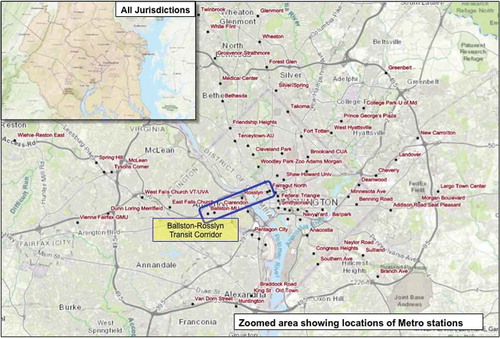
The TPB’s HHTS data includes a survey of 24 hour activity based travel patterns for 11,000 households in the greater Washington area, which includes northern Virginia and parts of Maryland. The survey was conducted between February 2007 and March 2008 and includes more than 25,000 person records, 16,000 vehicle records, and 130,000 trip records (MWCOG 2015). This activity-based survey data provides a wealth of trip information in diverse land uses in several jurisdictions within the MWCOG area (Figure 1).

Figure 1. Jurisdictional boundaries of TPB 2008 travel survey, MWCOG modeled area and metro stations.

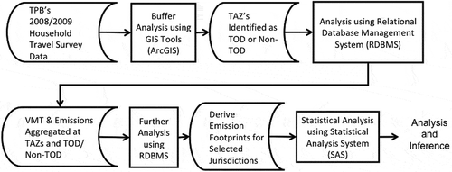
Data mining techniques for travel survey databases outlined by Venigalla, Chalumuri, and Mandapati (2005) are used in reducing HHTS database. The complete data reduction process and analysis steps are illustrated in Figure 2.

Figure 2. The travel survey based emission footprint analysis process.

3.1 Land use grouping

Most TAZs designated as TOD contain mixed-use developments located within comfortable walking distance of Metro stations. For example, Rosslyn-Ballston transit corridor in Arlington, Virginia and Bethesda suburb of Maryland (see Figure 1) have compact developments and are served by several Metrorail stations. Though the degree to which mixed-use land use around the Metrorail stations varies with the location of station, for this analysis it is assumed that through self-selection all TAZ’s within the specified radii of Metro rail stations are of TOD land use. It is important to note here that not necessarily every 0.5-mile buffer around each of the 96 Metro stations in the region is a TOD. However, these buffers are denoted as TODs for the purposes of demonstrating the effectiveness of the methodology. However, to alleviate the potential for underestimation of walking distance by Euclidian buffers, network walking-distance buffers would be preferable over Euclidean buffers.

Examination of HHTS data indicates that vehicle ownership is much less in TOD zones than the Non-TOD zones (Figure 3). To further examine the extent of personal automobile usage in TOD zones with respect to detailed travel mode, a comparative analysis of TOD vis-à-vis Non-TODs is performed. It is important to note that the TOD trips include trips that are either within a TOD zone or only one trip end is inside a TOD zone. However, Non-TOD trips only include trips that are completely outside a TOD zone.

Figure 3. Vehicle ownership in the TOD and non-TOD zones.

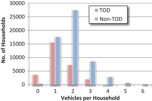
Aggregate analysis of the survey data showed that percentage usage of auto travel within Non-TOD zones far exceeds the same for TOD zones. It is noteworthy that personal vehicle usage is higher than transit usage inside for both Non-TOD and TOD zones. A primary contributing factor for this observation may be that the TOD zone data includes trips with one trip-end in a Non-TOD zone. In other words, while the trip origin may be in a TOD zone, the trip destination may be in a Non-TOD zone. This is a testament to the fact that even though the MWCOG area enjoys one of the widely used public transit systems in United States, it’s lack of complete service coverage to all areas of MWCOG results in higher use of vehicle mode even in TOD areas.

3.2 Grouping for jurisdictional analysis

At the time of TPB’s conducting HHTS in 2007/2008, Metrorail served six local jurisdictions: District of Columbia, City of Alexandria and Counties of Arlington, Fairfax, Montgomery and Prince George’s County (see Figure 1). Several other suburban and exurban counties, which were not served by Metrorail at that time of the survey, are also included in the analyses. Treated as Non-TOD land uses, these counties include Anne Arundel, Charles, Fauquier, and Stafford (Exurban); and Howard and Prince William (Suburban). Table 1 presents the complete list of jurisdictions and their urban classification included in the overall analysis.

Table 1. MWCOG jurisdictions and their urban classification.

Census FIPs	Jurisdiction	Abbreviation	Urban Classification
24,003	Anne Arundel County	AAC	Exurban
51,013	Arlington County	AC	Urban Core
24,017	Charles County	CC	Exurban
51,510	City of Alexandria	CA	Urban Core
11,001	District of Columbia	DC	Urban Core
51,059	Fairfax County	FFC	Suburban
51,061	Fauquier County	FqC	Exurban
24,027	Howard County	HC	Suburban
51,107	Loudoun County	LC	Not classified
24,031	Montgomery County	MC	Suburban
24,033	Prince George’s County	PGC	Suburban
51,153	Prince William County	PWC	Suburban
51,179	Stafford County	SC	Exurban
-	Other Rural counties	OC	Other Rural

4 Household VMT

Travel distances of all trips made using automobiles were first aggregated at the household level. The household-level vehicle miles of travel (VMT) were then weighted by the household sample weight. This step is then followed with derivation of the weighted averages of VMT per household for each of the study jurisdictions listed in Table 1. Travel metrics for TAZs within 0.5-mile and 0.25-mile radii of all metro stations are computed separately (Table 2).

Table 2. Average household vehicle miles of travel (VMT/hh).

	Radius from Metro Rail Stations
	0.25 miles		0.50 miles
City/County	Non-TOD (outside)	TOD (inside)	Non-TOD (outside)	TOD (inside)
Anne Arundel County	58.29		58.29
Arlington County	33.46	35.04	29.24	38.41
Charles County	85.80		85.80
City of Alexandria	27.97	31.34	29.23	27.65
District of Columbia	28.22	24.38	30.26	24.57
Fairfax County	49.36	37.01	49.74	37.53
Fauquier County	121.20		121.20
Howard County	57.63		57.63
Loudoun County	81.75		81.75
Montgomery County	48.95	31.55	51.41	34.81
Prince George’s County	53.48	41.76	54.19	43.56
Prince William County	67.83		67.83
Stafford County	64.88		64.88

● Bold emphasis indicates a counter-intuitive occurrence where VMT/hh is lower for Non-TOD than for TOD.

● Shaded cells indicate that there is no metro rail service in the jurisdiction.

Intuitively it would be expected that VMT per household in Non-TOD areas would be higher than the same for the TOD counterparts for the same jurisdiction. However this is not the case for both Arlington County and City of Alexandria (Table 2). For both 0.25 mile and 0.50 mile radii TODs, travel characteristics of Arlington County residents living in TODs have higher VMT per household than those living in Non-TODs. The same counter-intuitive trend is visible for the 0.25 mile radius TODs of City of Alexandria.

This counter-intuitive trend could be because the definition of TOD for some Metro stations in these two jurisdictions may not be apt. However, there is a plausible explanation for this trend. A careful examination of the HHTS trips indicated a significant portion of the survey respondents living in the TOD zones of Arlington County and City of Alexandria reported fairly long reverse-commute trips (trips that are headed against the direction of peak traffic flow). For example, several TOD residents of Arlington County took 50 miles or longer auto trips to suburban and exurban counties such as Anne Arundel County, Spotsylvania County, Frederick City (Maryland) and Frederick County (Virginia) and Loudoun County. These long reverse-commute trips skewed the household VMT of 0.25-mile TOD zones in both Arlington County and City of Alexandria. Furthermore, these trips indicate the deficiency in transit network for the residents of Arlington County who commute to other jurisdictions in the modelled area. The VMT differences are consistent with conclusions by Zhang et al. (2012), which stated VMT in the TOD areas tend to be less than VMT in Non-TOD areas by up to 38% in the Washington D.C. area and 21% in Baltimore with otherwise similar land use patterns.

Table 3 presents VMT per household consolidated for three major urban classifications identified in Table 1. When Arlington County is excluded, household-level VMT for Non-TOD zones far exceeds that of the TOD zones, which confirms intuition.

Table 3. Average household vehicle miles of travel (VMT/hh) by urban class.

	Radius from Metro Rail Stations
	0.25 miles		0.50 miles
Urban Classification	Non-TOD (outside)	TOD (inside)	Non-TOD (outside)	TOD (inside)
Exurban Counties	76.76	-	76.76	-
Suburban Counties	55.15	36.20	56.35	38.07
Urban Core (Incl. Arlington)	29.42	26.89	29.75	27.51
Urban Core (Excl. Arlington)	28.15	25.00	29.94	24.96

5. Emission footprints of household automobile travel

The approach to emission footprint analysis combines the VMT values derived in the previous section and aggregate emission rates developed for the MWCOG region shown Table 4 (MWCOG, 2016).

Table 4. Emission rates (gm/mile) used in the 2016 CLRP (MWCOG 2016).

Year	Ozone VOC	Ozone NOx	PM2.5 Direct	Precursor NOx
2016	0.337	0.407	0.02	0.45
2017	0.301	0.301	0.01	0.34
2025	0.204	0.142	0.01	0.16
2030	0.139	0.081	0.01	0.10
2040	0.098	0.043	0.01	0.06

The emission footprints (in grams per household) of each pollutant for each of the TOD and Non-TOD land use areas are then computed using Equation 1.

(1) $e_{p,lt}=\sum _z\left(\frac{{\sum }_{hh}\left(VM{T}_{lt,z,hh}\times e{r}_p\times W{t}_{hh}\right)}{{\sum }_{hh}\left(W{t}_{hh}\right)}\right)/\sum _z\left(\frac{{\sum }_{hh}\left(VM{T}_{lt,z,hh}\times W{t}_{hh}\right)}{{\sum }_{hh}\left(W{t}_{hh}\right)}\right)$(1)

Where:

$e_{p,lt}$ = Emission footprints (gram/household) of pollutant type p, for land use type lt;

$VM{T}_{lt,z,hh}$= Vehicle Miles of Travel for zone z in land use category lt and household hh;

p = Pollutant type (Ozone VOC, Ozone NOx, PM_2.5 Direct and Precursor NOx);

$e{r}_p$ = Emission rates (2016) shown in Table 4; and

$W{t}_{hh}$ = Household weight in the travel survey data.

As shown in Figure 2, which illustrates various steps in the study process, results of the sample means analysis for each of the selected area were post-processed to derive emission footprints of Ozone VOC, Ozone NOx, and PM_2.5 Direct by facility type and area type. Table 5 presents the summary results of emission analysis for Ozone VOC. (Results and conclusions for Ozone NOx, PM2.5 Direct and Precursor NOx, are similar to that of Ozone VOC and hence not shown in this paper).

Table 5. Average ozone VOC emissions per household (grams/hh).

	Radius from Metro Rail Stations
	0.25 miles		0.50 miles
County	Non-TOD (outside)	TOD (inside)	Non-TOD (outside)	TOD (inside)
Anne Arundel County	19.64		19.64
Arlington County	11.28	11.81	9.85	12.95
Charles County	28.92		28.92
City of Alexandria	9.43	10.56	9.85	9.32
District of Columbia	9.51	8.22	10.20	8.28
Fairfax County	16.63	12.47	16.76	12.65
Fauquier County	40.84		40.84
Howard County	19.42		19.42
Loudoun County	27.55		27.55
Montgomery County	16.50	10.63	17.32	11.73
Prince George’s County	18.02	14.07	18.26	14.68
Prince William County	22.86		22.86
Stafford County	21.86		21.86

● Bold emphasis indicates a counter-intuitive occurrence where VMT/hh is lower for Non-TOD than for TOD.

● Shaded cells indicate that there is no metro rail service in the jurisdiction.

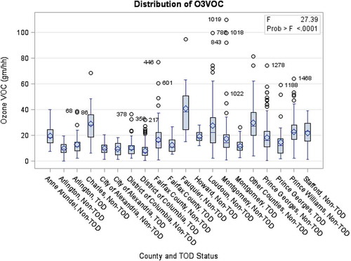
It can be seen that the mean emission footprints attributable to personal auto travel for Non-TOD areas are generally higher than the footprints for TOD areas. However, NON-TOD land uses in Arlington County bucked this trend for all pollutants. This is to be expected because, as revealed in VMT analysis (Table 5), significant portion of household auto trips of the TOD land uses of Arlington County appear to be engaged in reverse commute trips of 50-miles or longer. Figure 4 illustrates means and quartiles of emission footprints Ozone VOC for across the model’s class variables. It is observed that emission footprints for Non-TODs land uses are generally higher than the footprints for TODs. Note that only 0.25-mile radius TODs are shown in Figure 4.

Figure 4. County-specific ozone VOC emission footprints.

5.1 Land use means comparison: non-TOD vs. TOD

Despite the noticeably higher emission footprints of Non-TOD land uses; it is not known if these differences are statistically significant. Hypotheses tests were conducted on mean values of emission footprints presented in Table 5. Student’s t-test is one of the most commonly used statistical significant tests for means comparison (Rathi & Venigalla, 1992). The selection of households in the TPB travel survey data used in this analysis was done at random, which meets one of the criteria for t-test. Assuming that the VMTs associated with travel for the households are normally distributed, two-sample t-test would be appropriate for testing the following hypotheses:

Null Hypothesis, H₀:

${\mu }_{non-TOD,i}-{\mu }_{TOD,j}=0;$

Alternate Hypothesis, H_a:

${\mu }_{non-TOD,i}-{\mu }_{TOD,j}>0;$ (One-tailed)

${\mu }_{non-TOD,i}-{\mu }_{TOD,j}\ne 0;$ (Two-tailed)

Where:

${\mu }_{non-TOD,i}$ = Mean of emission footprint for a given Non-TOD area, i; and

${\mu }_{TOD,j}$ = Mean of emission footprint for a given TOD area, j.

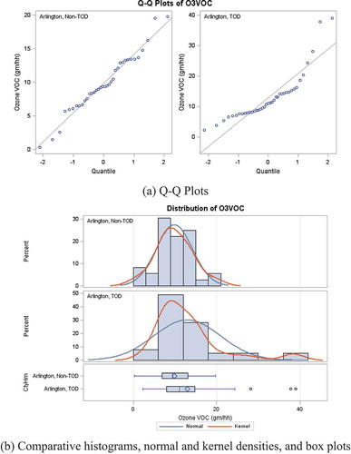
To test for Normality, mean values of emission footprints were also tested for Normal distribution assumption. Figure 5 provides a representative illustration of these tests for Non-TOD vs. TOD emission footprints of Ozone VOC for Arlington County. The figure indicates that Ozone VOC household-level emission footprints for both Non-TOD and TOD in Arlington County are normally distributed. Similar tests were conducted for all counties considered in the analysis (not shown). The tests for Normality of emission household footprints of all four pollutants (namely, Ozone VOC; Ozone NOx; PM 2.5 Direct; and Precursor NOx) and for all TAZs across all counties confirmed that the footprints aggregated at TAZ-level are random and independently distributed. Therefore, t-test is an appropriate statistical test for pairwise comparisons of means of emission footprints. Using the t-test procedure in the Statistical Analysis System (SAS) software, pairwise comparisons were made on sample means for Non-TOD and TOD areas of the same jurisdiction. Specifically, differences in emission footprints for Ozone VOC, Ozone NOx, PM2.5 Direct and Precursor NOX attributable to Non-TOD and TOD land uses for TAZs in six jurisdictions served by Metro rail service, namely, District of Columbia, City of Alexandria and Arlington, Fairfax, Montgomery, Prince George’s counties were analysed.

Figure 5. Test for normality of ozone VOC distribution across non-TOD and TOD TAZs.

Mean differences of Ozone VOC emission footprints and the associated statistics on 95% confidence intervals, degrees of freedom (DF), t-values and probability of Type II errors for the both pooled (equal variance) and Satterthwaite methods (unequal variances) are shown in Table 6. The confidence limits shown for the standard deviations are of the equal-tailed variety.

Table 6. Two-sample t-test results for ozone VOC emission footprints.

Non-TOD vs. TOD Sample Means Tested	Var. Method	^1Mean Diff. (gm/mi)	95% CL Mean Diff.		DF	t Value	Pr > |t|
District of Columbia	Pooled	1.9180	0.2026	3.6333	213	2.20	0.0286
	Satterthwaite	1.9180	0.1446	3.6913	124.21	2.14	0.0343
Arlington County	Pooled	−3.0920	−6.0744	−0.1095	73	−2.07	0.0424
	Satterthwaite	−3.0920	−6.0208	−0.1631	59.804	−2.11	0.0389
City of Alexandria	Pooled	0.5348	−2.1700	3.2396	51	0.40	0.6931
	Satterthwaite	0.5348	−2.2772	3.3469	38.42	0.38	0.7025
Fairfax County	Pooled	4.1152	0.4057	7.8247	280	2.18	0.0298
	Satterthwaite	4.1152	1.5788	6.6516	43.292	3.27	0.0021
Montgomery County	Pooled	4.1152	0.4057	7.8247	244	3.34	0.0010
	Satterthwaite	4.1152	1.5788	6.6516	242.6	4.66	<.0001
Prince George’s County	Pooled	3.5826	−0.0608	7.2259	257	1.94	0.0539
	Satterthwaite	3.5826	−0.2107	7.3758	62.301	1.89	0.0637

● Bold emphasis indicates that the difference in sample means of the two land uses is not statistically significant at α = 5%.

● ¹ Negative value for ‘Mean Diff.’ indicates that emission footprints for Non-TOD TAZs are higher than footprints for TOD TAZs.

As Table 6 indicates, statistically significant differences exist between the TAZ-specific emissions footprints of TOD and Non-TOD land uses for Arlington, Fairfax and Montgomery counties and District of Columbia. However, the same cannot be said about Prince George’s County (PGC) and City of Alexandria. The probability of Type-II error for PGC is less than 0.10, or the difference is significant at α = 10%. Analysis of mean differences of Ozone NOx, PM2.5 Direct and Precursor NOx emission footprints between Non-TOD and TOD yielded similar results and are not presented in this paper.

For all pollutants, there is no statistically significant difference between the emission footprints for Non-TOD and TOD for the City of Alexandria. This may be attributable to unique nature of land use within Alexandria. Thus, it may be concluded that for Fairfax, Montgomery and Prince George’s counties, and District of Columbia emission footprints of TOD land uses are significantly lower than the footprints for Non-TOD land uses. However, Arlington County bucked the trend with higher emission footprints for TOD than the footprints for Non-TOD TAZs. Furthermore, it appears that in City of Alexandria the emissions for TOD zones are comparable to that of Non-TOD zones.

5.2 All pairwise means comparisons: jurisdiction and land use

Previous section provided pairwise comparisons of emission footprints for Non-TOD and TOD land uses within the same jurisdictions, which are served by Metrorail. However, from academic and policy perspectives, it is useful to find out similarities and differences between pairs of jurisdictions and land uses across the region. Due to the sheer number of pairwise comparisons possible for all class variables included in the analyses (Table 1) and their Non-TOD/TOD designates, where applicable, it is not practical to use Student’s t-test for identifying those similarities or dissimilarities.

When numerous pairwise means comparisons are to be made, the most commonly used test of significance for all pairwise comparison is Tukey’s Range Test (TRT). TRT is normally performed in combination with analysis of variance methods. However, TRT assumes equal variance of samples whose means are compared. To verify if TRT is suitable for pairwise comparisons across jurisdictions, tests of equality of variance variances for select pairs of Non-TOD and TOD land uses were performed. The results of this equality of variance tests using Folded F Method are summarized in Table 7.

Table 7. Equality of variances using folded F method.

Non-TOD vs. TOD Means Comparison for:	Num DF	Den DF	F Value	Pr > F
Arlington County	38	35	3.34	0.0005
City of Alexandria	20	31	1.34	0.4514
District of Columbia	68	145	1.18	0.4169
Fairfax County	254	26	2.80	0.0027
Montgomery County	174	70	7.30	<.0001
Prince George’s County	44	213	1.08	0.7003

Bold emphasis indicates that the equal variance assumption between sample pairs may not be accurate.

TRT provides reliable answers when population variances are similar. However, statistics shown in Table 7 are inconclusive as only three of the six pairs tested showed that variances of emission footprints for all TAZs across all counties are equal. However, given the random sampling of HHTS and normality of distribution of emissions footprints, for the purpose of all pairwise comparisons it is assumed that TRT would be applicable.

Using emission footprints as response variables and individual jurisdictions (i.e. counties) and their urban classification as class variables, General Linear Models procedure in SAS (PROC GLM) was performed along with associated TRT for nearly 200 possible pairs. The results from the analysis are consolidated into an easy to read chart shown in Figure 6.

Figure 6. County-by-county pairwise comparisons for ozone VOC emission footprints.

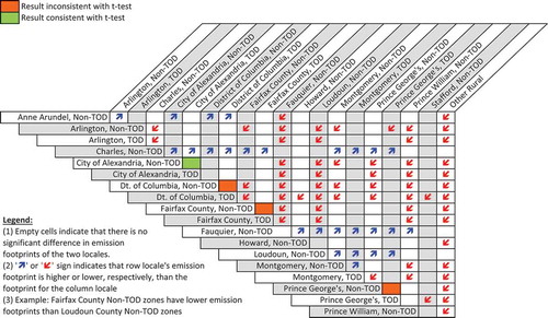
A general observation from Figure 6 is that emission footprints for ‘exurban’ and other ‘rural counties’ are significantly higher than their suburban and urban counterparts. As this observation itself is not surprising, the procedures and statistical methods used in developing this comparative assessment between pairs of jurisdictions within a region may be invaluable in policy-making exercises related to air quality monitoring. As mentioned earlier this comparative chart would be identical for other three pollutants analyzed, due mainly to their direct proportionality with VMT.

However, as also highlighted in Figure 6, notable disagreements are observed between the results of student’s t-test and TRT. For example, student t-test observed statistically significant difference between Non-TOD and TOD zones of Arlington and District of Columbia where as TRT indicated that these differences are not significant. Because the results of equal variance analysis (Table 7) are inconclusive, the results of TRT may be less reliable. Therefore, more appropriate statistical test for all the 190 pairwise comparisons shown in Figure 6 is the student t-test. Regardless of the test, the method described would be useful in sketch planning and/or policy analysis requiring comparative assessment of land use types, jurisdictions or any other classification.

6. Conclusions and recommendations

A simple methodology to derive household level emission footprints of auto trips from travel survey databases was developed, applied on household travel survey data for Washington DC Metro area. The study also offered statistical methods to validate comparative assessments of emission footprints between pairs of land use types and municipal jurisdictions. Pairwise comparisons of means using Student’s t-test between TOD and Non-TOD areas in the Metro Washington DC area indicated that for all but one jurisdiction emission footprints for Non-TOD zones are significantly higher than the footprints for TOD zones. The only anomaly to this conclusion is Arlington County, where emission footprints for TOD are higher than the Non-TOD footprints. This anomaly may be attributable to long reverse commute trips originating from the TOD zones of Arlington County.

This study demonstrated an innovative use of household travel survey data for making comparative assessment of emission footprints by land use and jurisdiction. The methods and results presented in the study would be useful primarily in sketch planning and/or policy analysis requiring comparative assessment of land use types, jurisdictions or any other classification. Furthermore, the emission footprints derived from periodic travel surveys would establish baseline for comparison with future emission footprints. For example, when the 2018 HHTS survey data for MWCOG area are available in the year 2020, emission footprints from the 2018 data may be compared to 2008 footprints. These comparison studies can include identifying trends and changes in emission footprints that may be attributed to land use policy changes.

After the initial effort of computing TAZ-level emission footprints, they can be stored in a simple spreadsheet, which can then be aggregated at whatever geographic grouping that may be appropriate. Thus, these footprints could serve as baseline for comparing across spatial and temporal dimensions.

Acknowledgments

This study is partially funded by the US Department of Transportation under the University Transportation Centres program. The authors are grateful for thorough review and valuable suggestions provided by dissertation committee members Dr. Girum Urgessa, Shanjiang Zhu, Dr. Jie Xu and Dr. Laura Kosoglu of George Mason University. The authors also express their gratitude for four anonymous reviewers whose thorough review of the manuscript and comments helped improve this paper significantly.

Disclosure statement

No potential conflict of interest was reported by the authors.

Additional information

Funding

This work was supported by the University Transportation Centers program of FHWA.

References

- Cervero, R. (1993). Ridership impacts of transit-focused development in California. Berkeley, CA: University of California at Berkeley Institute of Urban and Regional Development.
- Cervero, R. (2006). Alternative approaches to modeling the travel-demand impacts of smart growth. Journal of the American Planning Association, 72(3), 285–295.
- Cervero, R., & Murakami, J. (2010). Effects of built environments on vehicle miles traveled: Evidence from 370 US urbanized areas. Environment and Planning A, 42, 400–418.
- Chalumuri, S., & Venigalla, M. M. (2004). Methodology for deriving vehicle activity parameters from travel survey databases. Transportation Research Record: Journal of the Transportation Research Board, 1880, 108–118.
- Chatterjee, A., Reddy, P. M., Venigalla, M. M., & Miller, T. (1996). Operating mode fractions on urban roads derived by traffic assignment. Transportation research record. Journal of the Transportation Research Board, 1996(1520), 97–103.
- Crowley, D., Shalaby, A., & Zarei, H. (2009). Access walking distance, transit use, and transit-oriented development in North York City Center, Toronto, Canada. Transportation Research Record: Journal of the Transportation Research Board, (2110), 96–105.
- Danieau, J. (2009). Emission benefits from alternative land use development (phase I). Transportation, Land Use, Planning, and Air Quality. American Society of Civil Engineers., 1–0, 51–61.
- Dixit, S. (2017, August 2017). Modeling emission footprints of sustainable land use policies at local jurisdictional level. A dissertation submitted in partial fulfillment of requirements for doctor of philosophy degree. George Mason University.
- Ewing, R., Bartholomew, K., Winkelman, S., Walters, J., & Chen, D. (2007). Growing cooler: The evidence on urban development and climate change. Washington, DC: Urban Land Institute.
- Ewing, R., & Cervero, R. (2001). Travel and the built environment: a synthesis. Transportation Research Record: Journal of the Transportation Research Board,1780, 87–114. doi:10.3141/1780-10
- Ewing, R., & Cervero, R. (2010). Travel and the built environment: A meta-analysis. Journal of the American Planning Association, 76, 265–294.
- Faghri, A. (2012, May). Advanced planning models for transit-oriented developments (Dissertation). George Mason University.
- Faghri, A., & Venigalla, M. M. (2013). Measuring travel behavior and transit trip generation characteristics of transit-oriented developments. Transportation Research Record. Journal of Transportation Research Board., 2397, 72–79.
- Faghri, A., & Venigalla, M. M. (2016). Disaggregate models for mode choice behavior of transit-oriented developments. Paper presented at the 95th Annual Meeting of the Transportation Research Board. Washington, DC. Transportation Research Board.
- Frank, L. D., Stone, B., Jr, & Bachman, W. (2000). Linking land use with household vehicle emissions in the central puget sound: Methodological framework and findings. Transportation Research Part D: Transport and Environment, 5(3), 173–196.
- Handy, S. (2005). Smart growth and the transportation-land use connection: What does the research tell us? International Regional Science Review, 28, 146–167.
- Iacono, M., Levinson, D., & El-Geneidy, A. (2008). Models of transportation and land use change: A guide to the territory. Journal of Planning Literature, 22, 323–340.
- Krimmer, M. J., & Venigalla, M. M. (2006). Measuring impacts of high-occupancy-vehicle lane operations on light-duty-vehicle emissions: Experimental study with instrumented vehicles. Transportation Research Record: Journal of the Transportation Research Board, 1987, 1–10.
- Mathez, A., Manaugh, K., Chakour, V., El-Geneidy, A., & Hatzopoulou, M. (2013). How can we alter our carbon footprint? Estimating GHG emissions based on travel survey information. Transportation, 40(1), 131–149.
- Megenbir, L. E., & Habib, M. A. (2015). Estimating fuel consumption and vehicle emissions using multi-year travel survey data. Presented at 94th Annual Meeting of the Transportation Research Board, Washington, DC.
- Metro Washington Council of Governments (MWCOG). (2010). 2007/2008 TPB household travel survey: Technical documentation. Washington, DC: Metro Washington Council of Governments (MWCOG).
- Metro Washington Council of Governments (MWCOG). (2015). Air quality conformity analysis of the 2015 CLRP amendment and FY 2015–2020 TIP. Washington, DC: Metro Washington Council of Governments (MWCOG).
- Metro Washington Council of Governments (MWCOG). (2016, November). Financially constrained long-range transportation plan(CLRP) for the national capital region (Transportation Planning Board). Washington, DC: Author. http://www1.mwcog.org/clrp/resources/2016/2016AmendmentReport.pdf
- Nahlik, M. J. (2014). Transit-oriented smart growth can reduce life-cycle environmental impacts and household costs in Los Angeles. Transport Policy, 35, 21–30.
- Nasri, A., & Zhang, L. (2014). Assessing the impact of metropolitan-level, county-level, and local-level built environment on travel behavior: Evidence from 19 US urban areas. Journal of Urban Planning and Development, 141(3), 04014031 (1–10).
- O’Sullivan, S., & Morall, J. (1996). Walking distances to and from light-rail transit stations. Transportation Research Record, 1538, 19–26.
- Rathi, A. K., & Venigalla, M. M. (1992). Variance reduction applied to urban network traffic simulation. Transportation Research Record: Journal of the Transportation Research Board, 1365, 133–146.
- Shekarrizfard, M., Faghih-Imani, A., Tetreault, L.-F., Yasmin, S., Reynaud, F., Morency, P., Hatzopoulou, M. (2017). Modelling the spatio-temporal distribution of ambient nitrogen dioxide and investigating the effects of public transit policies on population exposure. Environmental Modelling & Software, 91, 186–198.
- Still, K., Seskin, S., & Parker, T. (2000). Chapter 3: How does TOD affect travel and transit use. In Caltrans statewide transit-oriented development study, 46–50. Sacramento: California Department of Transportation.
- Tayarani, M., Poorfakhraei, A., Nadafianshahamabadi, R., & Rowangould, G. M. (2016). Evaluating unintended outcomes of regional smart-growth strategies: Environmental justice and public health concerns. Transportation Research Part D: Transport and Environment, 49, 280–290.
- US Environmental Protection Agency (US EPA). (2018 January). Criteria Pollutants. Retrieved from https://www.epa.gov/criteria-air-pollutants
- Venigalla, M. M., Miller, T., & Chatterjee, A. (1995a). Start modes of trips for mobile source emissions modeling. Transportation Research Record, 26–34).
- Venigalla, M, Miller, T, & Chatterjee, A. (1995b). Alternative operating mode fractions to federal test procedure mode mix for mobile source emissions modeling. Transportation Research Record, 1472, 35–44.
- Venigalla, M., & Pickrell, D. (2002). Soak distribution inputs to mobile source emissions modeling: Measurement and transferability. Transportation Research Record: Journal of the Transportation Research Board,1815, 63–70.
- Venigalla, M. M. (2004, November). Household travel survey data fusion issues. In Resource Paper, National Household Travel Survey Conference: Understanding Our Nation’s Travel, 1(2). Retrieved from http://onlinepubs.trb.org/onlinepubs/archive/conferences/nhts/workshop-datafusion.pdf
- Venigalla, M. M., & Baik, B. (2007). GIS-based engineering management service functions. Journal of Computing in Civil Engineering, 21(5), 331–342.
- Venigalla, M. M., Chalumuri, S., & Mandapati, R. (2005). Developing custom tools for deriving complex data from travel survey databases. Transportation Research Record: Journal of the Transportation Research Board, 1917, 80–89.
- Venigalla, M. M., Chatterjee, A., & Bronzini, M. S. (1999). A specialized equilibrium assignment algorithm for air quality modeling. Transportation Research Part D: Transport and Environment, 4(1), 29–44.
- Venigalla, M. M., & Faghri, A. (2015). A quick-response discrete transit-share model for transit-oriented developments. Journal of Public Transportation, 18(3), 107–123.
- Venigalla, M. M., & Pickrell, D. (1997). Implications of transient mode duration for high resolution emission inventory studies. Transportation Research Record: Journal of the Transportation Research Board, 1587, 63–72.
- Zhang, L., Hong, J., Nasri, A., & Shen, Q. (2012). How built environment affects travel behavior: A comparative analysis of the connections between land use and vehicle miles traveled in US cities.