How accurate is the regional travel demand model in mimicking real-world travel times?

ABSTRACT

This paper provides insights pertaining to the validity of a regional travel demand model in mimicking real-world travel times. The estimated travel times from the regional travel demand model, for the base year 2015, for Mecklenburg County in the city of Charlotte, North Carolina (NC) were compared with travel time statistics from a private data source, for the same year. The results indicate that the estimated travel times from the regional travel demand model are typically lower than the 85^th percentile travel times, irrespective of the link speed limit. The estimated travel times for the Central Business District (CBD) area type are moderately correlated with the travel time statistics from the private data source, irrespective of the time of the day. For all the other area types, stronger correlations were observed when the estimated travel times from the regional travel demand model are compared with 10^th to 50^th percentile travel times. The calculated Pearson correlation coefficients are low for morning and evening peak periods compared to mid-day and night-time period, indicating the inability of the regional travel demand model in mimicking congested traffic conditions accurately.

KEYWORDS:

• Travel time
• regional travel demand model
• speed limit
• time of the day
• area type

Introduction

Travel demand forecasting is a process which helps in the estimation of the future trends in travel patterns as well as the travel times, using current trends in travel patterns and travel times. Transportation planners and system managers work to estimate future travel demand as well as to effectively manage the current travel demand for a transportation system. Metropolitan transportation plans and long-range transportation plans are developed for a region using outputs from the travel demand forecasting process. These plans contribute to the efficiency of the transportation system, improve mobility, reduce congestion, and has an indirect effect on other aspects such as air pollution.

The traditional regional travel demand forecasting process of a metropolitan area is a four-step process. The region is typically divided into various traffic analysis zones (TAZs) based on the socio-economic and demographic data. These TAZs should exhibit homogenous trip making patterns (Meyer & Miller, 2000). After a rigorous feedback process involving calibration of trip generation, trip distribution, mode split, and trip assignments steps, the travel time, link volume, and volume-to-capacity ratio (V/C) are estimated for each link, typically on major roads, in the network. The regional travel demand model predicts the link flow and travel time based on the routes and mode opted by the traveler from an origin to the destination (Florian & Hearn, 1995). The algorithm used for trip assignment is of no use if the resulting flow does not match with the observed flow (Tobin, 1979).

Trips are traditionally assigned based on Wardrop’s first principle for equilibrium flows (Wardrop, 1952). Many algorithms were developed to satisfy the equilibrium flow condition. Nguyen (1974), LeBlanc (1973), Dafermos (1971), and Bruynooghe and Gilbert (1968) outline a few example algorithms that work with a fixed origin-destination matrix for a road network. Slavin et al. (2006) compared different approaches to compute outputs from the user equilibrium trip assignment method. Their results showed that the origin-based approach congregates more than other considered approaches. Dial (1971) developed a path-based user equilibrium algorithm, that shifted the flow from the costliest path to the cheapest path.

Similarly, Bell & Cassir (2002) developed user equilibrium traffic assignment method based on game theory. For equilibrium condition, the probability of selection of each path is the same i.e., the cost is the same. The model distributed the flow based on minimum trip cost during the congested and uncongested period. Lo & Chen (2000) used Facchinei & Soares (1997) gap function for addressing the traffic equilibrium problem. They developed a model to fulfill 1) traffic assignment based on general route cost structure, and 2) to ensure that every point of minimization corresponds to an overall minimum. The vast and abundant literature on travel demand forecasting process and resulting outputs is an indicator of its significance with decision-making and developing transportation plans.

Travelers, on the other hand, plan their trip based on trip purpose, mode, travel time, travel cost, and route. The flow pattern in an urban network depends on two mechanisms. It depends on the route selected by a traveler to minimize the travel time from an origin to the destination. It could also depend on congestion, which can be explained as the use of the transportation system. A good regional travel demand model should predict the traveler’s choices with accuracy (Carrion & Levinson, 2012).

The travel time helps travelers make decisions regarding route choice, departure time choice, and mode choice (if options are available). It varies by the time of the day, the day of the week, and season of the year. It also depends on factors that influence demand for travel (for example, an increase in gas price could decrease the demand for travel and therefore reduce travel time). The advancements in technology, growing awareness to make the world more sustainable, congestion pricing, and incentives to use alternate modes of transportation have a catalytic effect on the trip making patterns, and hence, travel demand, Therefore, the accuracy of the travel demand forecasting model in mimicking real-world conditions is often debated. The model could overestimate or underestimate outputs such as travel demand and travel time, if not calibrated considering accurate and appropriate data. A few times, decisions made in the past may not be applicable for future purposes.

In spite of their limitations, transportation planners and system managers rely heavily on travel demand forecast model outputs for developing metropolitan transportation plans, long-range transportation plans, and for evaluating large-scale transportation project alternatives. Researching the relationship between outputs from the regional travel demand model and real-world data could help these transportation planners and system managers make informed decisions, or proactively anticipate and work to address any limitations from such forecasts. Therefore, the focus of this paper is to evaluate the relationship between outputs from a regional travel demand model and travel time statistics based on real-world data by the time of the day.

Continuous travel time data, for all links along major roads, is needed to assess travel time statistics and compare with outputs from the regional travel demand model. Global Positioning Systems (GPS) installed in vehicles, commercial devices, and smartphone with apps are currently used to capture travel time information, in near real-time (Haghani et al., 2009). Many studies were conducted to compare the reliability and accuracy of such probe sourced data to collect travel times. The Federal Highway Administration (FHWA) conducted a study to compare the private and public source data as well as services (Turner et al., 2011). Kim & Coifman (2014) and Lindveld et al. (2009) compared the speed feed against the concurrent loop detector data. Kim & Coifman (2014) observed that INRIX speed data lags the loop detector speed data. Their results showed that a shortage in the INRIX (confidence score = 30) data affects the accuracy, especially during off-peak hours on arterial streets. Haghani et al. (2009) and Pulugurtha et al. (2015a, 2015b) compared INRIX travel time data with the data captured from Bluetooth detectors and other sources. The results from past research indicate that travel times are comparable for freeways, while caution must be exercised when using data for arterial streets.

The regional travel demand model network, typically, include major roads in the region. These include functional classes such as interstates, expressways, major and minor arterial streets, and some collector roads. The design standards, area type and speed limits along these road functional classes vary. The characteristics (lane width, shoulder width, number of lanes, grade, traffic volume and composition, ramps, etc.) that influence travel times on interstates and expressways differ from the characteristics that influence travel time on major and minor arterials (lane width, grade, traffic volume and composition, parking, bus-stops, intersection controls, driveways, signal phasing/timing, etc.). Therefore, investigating the relationship between outputs from the regional travel demand model and travel time statistics by speed limit (an indicator of road functional class) will provide valuable insights.

Land use characteristics influence traffic patterns. Trips generated from a TAZ are influenced by the surrounding land use characteristics. Matt et al. (2005) explored the activity-based and utilities-based theories to study the relationship between travel behavior and land use. Further, Bagley & Mokhtarian (2002) investigated the effect of a residential neighborhood on the travel pattern in the San Francisco Bay area, California. They accounted that, neighborhood type has little influence when variables like socio-demographic and lifestyle are considered. Similar results were examined by Crane & Crepeau (1998). The land use characteristics vary by area type. Therefore, investigating the relationship between outputs from the regional travel demand model and travel time statistics by area type will also provide valuable insights.

Methodology

The regional travel demand model data was obtained for the Metrolina region from the city of Charlotte Department of Transportation (CDoT). The regional network consists of ten counties, located in North Carolina and South Carolina. However, for this research, only Mecklenburg County, North Carolina was considered for analysis (due to access to travel time data).

The base regional travel demand model was developed by CDoT using demographic, socio-economic, land use, and on-network characteristics for the year 2015. It is calibrated by comparing with traffic volumes and travel times for selected links in the Metrolina region. The estimated travel times from the four-step process, for the year 2015, were obtained for each link within the region. CDoT adopted the user equilibrium approach as the trip assignment method.

The travel times are estimated using the four-step process, for the year 2015, for four different time periods. They are morning peak (6:30 AM to 9:30 AM), mid-day (9:30 AM to 3:30 PM), evening peak (3:30 PM to 6:30 PM), and night-time (6:30 PM to 6:30 AM) periods. The estimated travel times considered from the regional travel demand model for this research is the travel time for each time period.

The real-world raw travel time data, at the one-minute interval, was downloaded from the Regional Integrated Transportation Information System (RITIS) website and imported into Microsoft Structured Query Language (SQL) server for the year 2015. The raw travel time database includes the time of the day, the day of the week, link-based speed, sample size, link length, travel time, and score (30 indicates real-time data; 20 indicates real-time data across multiple segments; 10 indicates historical data). Only raw travel time samples with a score of 30 were used in this research. Data for Saturdays, Sundays, and federal holidays were excluded in this research.

For every Traffic Message Channel (TMC) or link, travel time statistics were then computed by the time of the day and day of the week. The raw travel time data obtained from the private data source is acquired from sources, such as traffic sensors, probe vehicles, and the smart dust network (Regional Integrated Transportation Information System (RITIS), 2018). Since the regional travel demand model estimates travel time for the four selected time periods during a weekday, the raw travel time data was processed to compute travel time statistics for the same time periods. As an example, travel time data for each link with a score of 30 during a weekday in the year 2015, from 6:30 AM to 9:30 AM, was used to compute travel time statistics for the morning peak period.

The travel time statistics considered for analysis in this research include minimum travel time (MinTT), average travel time (AvgTT), percentiles of travel times indicated as ‘TT’ followed by the number representing the percentile (TT05, TT10, TT25, TT50, TT75, TT85, TT90 and TT95), and maximum travel time (MaxTT). The estimated travel times from the regional travel demand model were integrated with the computed travel times from the private data source, using the TMC code, which is a common field in both the databases.

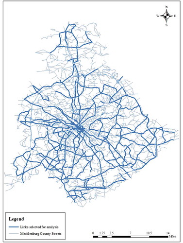
The length of a link (TMC) in the regional travel demand model and the private data source differ for some links. The difference between the link lengths was calculated. The links with a difference in link length greater than 0.1 miles were excluded from the analysis. Additionally, links with the speed limit equal to or less than 30 mph were also excluded from the analysis. Overall, 920 links with estimated travel times from the regional travel demand model and data to compute travel time statistics were considered in this research. Figure 1 shows the distribution of the links considered across the study area. The light-colored thin lines in the background indicate the street network of Mecklenburg County, NC.

Figure 1. Links considered for the analysis.

The speed limit of the links was considered in order to classify and analyze by the road functional class. Figure 2 represents the speed limit distribution of the links across the considered links. Majority of links with higher speed limit (greater than 50 mph) are present at the outer edges of the network whereas the links with moderate (>40 & ≤50 mph) and lower speed limits (>30 & ≤ 40 mph) are concentrated in the core/inner part of the network.

Figure 2. Distribution of the selected links by the speed limit.

Similarly, the area type was also considered to classify the links into different groups. The study area consisted of four area types; the Central Business District (CBD), fringe, urban, and suburban areas. In the regional travel demand model for the Metrolina region, the area types are calculated based on the residential and employment density within a 1.5-mile radius of the corresponding TAZ. The TAZ with population density (population/square mile) greater than or equal to 375 and an employment density (employment/square mile) below 2,600 is categorized as urban and suburban areas. The area type fringe is categorized as the TAZ with an employment density greater than 2,600 while CBD is categorized as the TAZ with an employment density greater than 10,500. Figure 3 represents the area type distribution of the considered links. The links in CBD and fringe area types are concentrated in the inner part of the network whereas the links in suburban, urban and rural area types are present at the outer parts and edges of the network.

Figure 3. Distribution of the selected links by the area type.

Scatter plots were generated to observe trends in the relationships. The Kolmogorov-Smirnov (K-S) test was performed to check for normality. If the test is not significant, then the data is said to be normally distributed. The significance value obtained for the sample size of 920 from the K-S test is greater than 0.05, indicating that the travel times are normally distributed for the selected time periods. Therefore, Pearson correlation coefficients were calculated to examine the relationships.

Pearson correlation coefficients were calculated between the estimated travel times from the regional travel demand model and the computed travel time statistics, for each time period, to check the degree of correlation between the two values. The calculated Pearson correlation coefficient is between −1.0 and +1.0. The Pearson correlation coefficient is considered to be very strong if the calculated value is closer to −1.0 or +1.0.

Three cases were considered for the analysis. In the first case, the Pearson correlation coefficients were calculated using data for all the links. In the second case, the Pearson correlation coefficients were calculated by categorizing data by the speed limit. They were also calculated by categorizing data by the area type in the third case. Due to the sample size constraints, the suburban and rural area types were considered as one category.

Plots showing trends in Pearson correlation coefficients, with the Pearson correlation coefficient on the y-axis and the travel time statistics on the x-axis, were generated. These plots were used to interpret the significance of the relationships and trends between the estimated travel times from the regional travel demand model and the computed travel time statistics from the private data source, by the time of the day, speed limit, and area type.

Results and discussion

Descriptive statistics such as the mean and standard deviation were first computed for the estimated travel times from the regional travel demand model and the travel time statistics, by the time of the day. Table 1 summarizes the means and standard deviations, by the time of the day, considering data for all the 920 links.

Table 1. Mean and standard deviation by time of the day – all links.

Measure	Morning Peak		Mid-day		Evening Peak		Night-time
	Mean	Std. Dev.	Mean	Std. Dev.	Mean	Std. Dev.	Mean	Std. Dev.
TT	2.18	1.62	2.02	1.42	2.15	1.92	1.39	1.04
MinTT	1.12	0.82	1.09	0.80	0.99	0.90	0.93	0.81
TT05	1.46	1.00	1.48	1.00	1.36	1.11	1.26	1.05
TT10	1.53	1.03	1.54	1.02	1.43	1.14	1.32	1.08
TT15	1.58	1.04	1.58	1.04	1.48	1.16	1.36	1.10
TT25	1.65	1.07	1.65	1.06	1.56	1.20	1.42	1.12
AvgTT	1.92	1.19	1.85	1.12	1.85	1.33	1.59	1.17
TT50	1.82	1.14	1.78	1.10	1.74	1.28	1.53	1.16
TT75	2.05	1.28	1.96	1.16	2.00	1.43	1.67	1.22
TT85	2.25	1.41	2.10	1.22	2.20	1.55	1.79	1.27
TT90	2.41	1.54	2.23	1.27	2.39	1.65	1.90	1.31
TT95	2.73	1.73	2.47	1.36	2.72	1.85	2.12	1.41
MaxTT	8.47	5.61	8.87	5.39	8.81	6.21	7.92	5.89

TT is estimated travel time from the regional travel demand model. All others are computed from the private data source.

The mean of the estimated travel times from the regional travel demand model (TT) is between the mean of the 75^th percentile travel time (TT75) and the 85^th percentile travel time (TT85) for the morning peak, mid-day, and evening peak periods. However, it is between the mean of the 15^th percentile travel time (TT15) and the 25^th percentile travel time (TT25) for the night-time period. The standard deviation of the estimated travel times from the regional travel demand model (TT) is greater than the standard deviation of the travel time statistics (in most cases, except for the maximum travel time, MaxTT) for the morning peak, mid-day, and evening peak periods.

To compare and assess the variations by the speed limit, the data were categorized into three groups. They are:

1. Speed limit >50 mph (85 links)

2. Speed limit >40 & ≤50 mph (592 links)

3. Speed limit >30 & ≤ 40 mph (243 links)

Descriptive statistics such as the mean and standard deviation were then computed for the estimated travel times from the regional travel demand model and the travel time statistics by the time of the day and speed limit. Table 2 summarizes the means and standard deviations by the time of the day and speed limit.

Table 2. Mean and standard deviation by time of the day and speed limit.

Speed Limit	Measure	Morning Peak		Mid-day		Evening Peak		Night-time
		Mean	Std. Dev.	Mean	Std. Dev.	Mean	Std. Dev.	Mean	Std. Dev.
>50 mph	TT	1.08	0.86	0.97	0.69	1.15	0.88	0.93	0.62
	MinTT	0.83	0.53	0.83	0.53	0.83	0.54	0.82	0.52
	TT05	0.89	0.58	0.89	0.58	0.90	0.59	0.88	0.56
	TT10	0.90	0.59	0.90	0.59	0.92	0.61	0.90	0.58
	TT15	0.92	0.60	0.91	0.60	0.93	0.62	0.91	0.58
	TT25	0.94	0.62	0.93	0.61	0.96	0.64	0.93	0.60
	AvgTT	1.09	0.97	0.98	0.66	1.17	0.79	0.98	0.63
	TT50	1.02	0.79	0.96	0.63	1.06	0.71	0.97	0.62
	TT75	1.16	1.27	1.00	0.67	1.25	0.93	1.00	0.65
	TT85	1.26	1.60	1.03	0.72	1.40	1.09	1.02	0.67
	TT90	1.35	1.97	1.07	0.78	1.52	1.23	1.04	0.69
	TT95	1.49	2.25	1.13	0.91	1.75	1.49	1.08	0.73
	MaxTT	10.61	10.47	9.43	8.89	10.76	8.43	11.78	9.97
>40 & ≤50 mph	TT	2.55	1.75	2.35	1.52	2.82	2.04	1.73	1.02
	MinTT	1.30	0.88	1.27	0.87	1.32	0.90	1.27	0.85
	TT05	1.69	1.07	1.70	1.06	1.75	1.09	1.63	1.04
	TT10	1.76	1.10	1.77	1.09	1.84	1.12	1.70	1.06
	TT15	1.81	1.11	1.81	1.10	1.90	1.14	1.75	1.08
	TT25	1.89	1.14	1.88	1.12	1.99	1.17	1.81	1.10
	AvgTT	2.18	1.26	2.10	1.18	2.32	1.29	2.00	1.15
	TT50	2.06	1.21	2.01	1.16	2.18	1.25	1.93	1.14
	TT75	2.32	1.33	2.20	1.22	2.48	1.38	2.09	1.18
	TT85	2.53	1.44	2.36	1.27	2.72	1.50	2.22	1.21
	TT90	2.71	1.54	2.49	1.32	2.93	1.60	2.34	1.25
	TT95	3.05	1.73	2.75	1.40	3.31	1.79	2.59	1.32
	MaxTT	8.80	4.82	9.24	4.74	9.98	5.82	8.76	5.61
≤ 40 mph	TT	1.67	1.09	1.59	1.01	1.82	1.26	1.30	0.77
	MinTT	0.78	0.55	0.76	0.53	0.79	0.56	0.78	0.54
	TT05	1.12	0.73	1.14	0.74	1.17	0.77	1.09	0.70
	TT10	1.19	0.75	1.21	0.76	1.25	0.80	1.15	0.72
	TT15	1.25	0.77	1.26	0.78	1.31	0.81	1.20	0.74
	TT25	1.33	0.79	1.33	0.79	1.40	0.84	1.26	0.76
	AvgTT	1.59	0.86	1.57	0.85	1.71	0.95	1.49	0.79
	TT50	1.50	0.84	1.49	0.83	1.60	0.91	1.41	0.79
	TT75	1.72	0.91	1.70	0.89	1.87	1.03	1.59	0.83
	TT85	1.90	0.97	1.85	0.93	2.09	1.14	1.74	0.87
	TT90	2.06	1.04	2.00	0.99	2.28	1.22	1.88	0.91
	TT95	2.36	1.15	2.27	1.07	2.62	1.37	2.16	1.01
	MaxTT	6.91	4.53	7.76	5.13	8.12	5.59	7.01	3.85

TT is estimated travel time from the regional travel demand model. All others are computed from the private data source.

When links with speed limit >50 mph are considered, the mean of the estimated travel times from the regional travel demand model (TT) is between the mean of the 50^th percentile travel time (TT50) and the 75^th percentile travel time (TT75) for the morning peak, mid-day, and evening peak periods. However, it is equal to the mean of the 25^th percentile travel time (TT25) for the night-time period.

When links with speed limit >40 & ≤50 mph are considered, the mean of the estimated travel times from the regional travel demand model (TT) is between the mean of the 85^th percentile travel time (TT85) and the 90^th percentile travel time (TT90) for the morning peak and evening peak periods. It is between the mean of the 75^th percentile travel time (TT75) and the 85^th percentile travel time (TT85) for the mid-day period, and between the mean of the 10^th percentile travel time (TT10) and the 15^th percentile travel time (TT15) for the night-time period.

When links with speed limit >30 & ≤ 40 mph are considered, the mean of the estimated travel times from the regional travel demand model (TT) is between the mean of the 50^th percentile travel time (TT50) and the 75^th percentile travel time (TT75) for the morning peak, mid-day, and evening peak periods. However, it is between the mean of the 25^th percentile travel time (TT25) and the 50^th percentile travel time (TT50) for the night-time period.

The standard deviation of the estimated travel times from the regional travel demand model (TT) and the travel time statistics in Table 2 are lower than those obtained when data for all the links are considered (Table 1).

The variations based on the area type was also assessed. The classification of the links based on the area type was used and are categorized into four classes:

1. Central Business District, CBD (96 Links)

2. Fringe (208 Links)

3. Urban (426 Links)

4. Suburban and Rural (190 Links)

The descriptive statistics for the links by the area type categories are also computed. Table 3 summarizes the means and standard deviations for the considered area types, by the time of the day. For the CBD area type, the mean of the estimated travel time is between the 25^th percentile travel time (TT25) and the 50^th percentile travel time (TT50) for the morning, mid-day and evening peak periods. However, the mean of the estimated travel time is between the 15^th percentile travel time (TT15) and the 25^th percentile travel time (TT25) for the night-time period.

Table 3. Mean and standard deviation by time of the day and area type.

Area Type	Measure	Morning Peak		Mid-day		Evening peak		Night-time
		Mean	Std. Dev.	Mean	Std. Dev.	Mean	Std. Dev.	Mean	Std. Dev.
CBD	TT	0.98	0.52	0.93	0.47	1.06	0.56	0.82	0.40
	MinTT	0.41	0.21	0.40	0.21	0.42	0.21	0.42	0.21
	TT05	0.65	0.34	0.65	0.33	0.66	0.34	0.63	0.33
	TT10	0.72	0.38	0.72	0.37	0.73	0.38	0.69	0.37
	TT15	0.76	0.41	0.76	0.39	0.78	0.41	0.74	0.39
	TT25	0.85	0.45	0.85	0.44	0.88	0.46	0.80	0.43
	AvgTT	1.10	0.54	1.08	0.53	1.17	0.56	1.05	0.52
	TT50	1.04	0.54	1.03	0.54	1.08	0.56	0.96	0.52
	TT75	1.25	0.63	1.22	0.63	1.33	0.66	1.16	0.60
	TT85	1.40	0.71	1.36	0.68	1.52	0.75	1.32	0.69
	TT90	1.54	0.78	1.49	0.73	1.68	0.80	1.48	0.77
	TT95	1.82	0.89	1.73	0.83	2.00	0.92	1.75	0.91
	MaxTT	5.59	2.89	6.50	3.43	6.32	3.13	6.73	3.87
Fringe	TT	1.81	1.13	1.72	1.07	2.02	1.32	1.30	0.73
	MinTT	0.85	0.51	0.83	0.50	0.87	0.51	0.83	0.49
	TT05	1.17	0.69	1.20	0.70	1.25	0.73	1.11	0.65
	TT10	1.24	0.72	1.27	0.73	1.33	0.78	1.18	0.68
	TT15	1.29	0.75	1.31	0.76	1.39	0.80	1.23	0.70
	TT25	1.37	0.78	1.38	0.78	1.48	0.84	1.29	0.73
	AvgTT	1.61	0.90	1.61	0.89	1.83	1.01	1.48	0.80
	TT50	1.52	0.86	1.53	0.85	1.69	0.95	1.41	0.78
	TT75	1.74	0.98	1.73	0.96	2.01	1.12	1.57	0.85
	TT85	1.91	1.07	1.89	1.04	2.26	1.25	1.70	0.92
	TT90	2.06	1.15	2.03	1.12	2.47	1.36	1.82	0.98
	TT95	2.34	1.29	2.28	1.25	2.87	1.58	2.05	1.09
	MaxTT	7.29	4.05	8.99	5.85	10.20	6.42	8.42	5.49
Urban	TT	2.47	1.68	2.30	1.46	2.72	1.94	1.70	0.97
	MinTT	1.23	0.78	1.19	0.75	1.24	0.79	1.19	0.74
	TT05	1.61	0.97	1.62	0.97	1.68	1.00	1.56	0.94
	TT10	1.69	1.00	1.69	0.99	1.76	1.04	1.63	0.97
	TT15	1.74	1.02	1.73	1.01	1.82	1.06	1.67	0.99
	TT25	1.82	1.06	1.80	1.04	1.91	1.10	1.74	1.01
	AvgTT	2.13	1.21	2.01	1.10	2.24	1.23	1.93	1.06
	TT50	2.00	1.14	1.93	1.08	2.11	1.18	1.85	1.04
	TT75	2.28	1.33	2.12	1.15	2.42	1.34	2.01	1.09
	TT85	2.50	1.49	2.27	1.20	2.66	1.47	2.15	1.14
	TT90	2.70	1.65	2.41	1.26	2.87	1.57	2.27	1.18
	TT95	3.05	1.87	2.66	1.34	3.23	1.78	2.52	1.27
	MaxTT	9.65	6.30	9.32	5.46	10.29	6.47	9.09	6.32
Suburban & Rural	TT	2.54	1.91	2.27	1.63	2.79	2.25	1.81	1.14
	MinTT	1.53	1.02	1.52	1.02	1.56	1.05	1.52	1.00
	TT05	1.86	1.23	1.87	1.23	1.90	1.26	1.81	1.20
	TT10	1.91	1.26	1.92	1.26	1.96	1.29	1.87	1.23
	TT15	1.95	1.28	1.95	1.28	2.00	1.31	1.91	1.24
	TT25	2.01	1.30	2.00	1.29	2.06	1.33	1.97	1.27
	AvgTT	2.22	1.42	2.16	1.36	2.30	1.45	2.11	1.32
	TT50	2.14	1.37	2.09	1.33	2.19	1.40	2.06	1.31
	TT75	2.30	1.46	2.22	1.39	2.40	1.53	2.17	1.36
	TT85	2.46	1.58	2.32	1.43	2.57	1.64	2.26	1.39
	TT90	2.60	1.70	2.42	1.48	2.73	1.73	2.35	1.42
	TT95	2.88	1.90	2.63	1.58	3.04	1.93	2.54	1.50
	MaxTT	8.54	5.73	8.90	5.24	8.87	5.45	8.52	6.08

TT is estimated travel time from the regional travel demand model. All others are computed from the private data source.

In case of the fringe area type, the mean of the estimated travel time is between the 75^th percentile travel time (TT75) and the 85^th percentile travel time (TT85) for the morning and evening peak periods. However, the means of the estimated travel time is between the 50^th percentile travel time (TT50) and the 75^th percentile travel time (TT75) for the mid-day period, and between the 25^th percentile travel time (TT25) and the 50^th percentile travel time (TT50) for the night-time period.

For the urban area type, the mean of the estimated travel time is between the 75^th percentile travel time (TT75) and the 85^th percentile travel time (TT85) for the morning peak period. However, the mean of estimated travel time is between the 85^th percentile travel time (TT85) and the 90^th percentile travel time (TT90) for the mid-day and evening peak periods. The mean of the estimated travel time for the night-time period is between the 15^th percentile travel time (TT15) and the 25^th percentile travel time (TT25).

For the suburban and rural area type, the mean of the estimated travel times is between the 85^th percentile travel time (TT85) and the 90^th percentile travel time (TT90) for the morning peak period. However, it is between the 90^th percentile travel time (TT90) and the 95^th percentile travel time (TT95) for the evening peak period. Likewise, the means of the estimated travel time lies in between the 75^th percentile travel time (TT75) and the 85^th percentile travel time (TT85) for the mid-day period. It is equal to the mean of the computed 25^th percentile travel time (TT25) for the night-time period.

Scatter plots were generated for all the speed limit categories for all the times of the day to examine general trends and distribution of samples with the estimated travel times from the regional travel demand model on the y-axis and the travel time statistic on the x-axis. Figures 4–6 show the distribution of samples by the speed limit category with the estimated travel times from the regional travel demand model on the y-axis and the 50^th percentile travel time (TT50) from the private data source on the x-axis. Best-fit line was added in each scatter plot to indicate the general data trend.

Figure 4. Scatter plots for the links with speed limit > 50 mph by time of the day.

Figure 5. Scatter plots for the links with speed limit > 40 & ≤ 50 mph by time of the day.

Figure 6. Scatter plots for the links with speed limit >30 & ≤40 mph by time of the day.

Figure 4(a–d) presents the scatter plots for the links with the speed limit > 50 mph. The estimated travel times from the regional travel demand model are greater than the 50^th percentile travel time (TT50) from the private data source for a majority of the links during the morning peak, mid-day, and evening peak periods. However, they are relatively closer to each other for most of the links during the night-time period.

Figure 5(a–d) presents the scatter plots for the links with the speed limit > 40 & ≤ 50 mph. The estimated travel times from the regional travel demand model are greater than the 50^th percentile travel time (TT50) from the private data source for a majority of the links during the morning peak, mid-day, and night-time periods. However, the estimated travel times from the regional travel demand model are lower than the 50^th percentile travel time (TT50) from the private data source for a majority of the links during the evening peak period. Figure 6(a–d) presents the scatter plots for the links with the speed limit >30 & ≤ 40 mph.

The estimated travel times from the regional travel demand model are greater than the 50^th percentile travel time (TT50) from the private data source for a majority of the links irrespective of the time of the day.

The generated scatter plots with best-fit lines indicate that the relationships between the estimated travel times from the regional travel demand model and travel time statistics from the private data source are linear in nature. While the general trend is linear, the number of links for which the estimated travel times from the regional travel demand model are greater than, equal to, or less than the travel time statistics varies by the posted speed limit and time of the day.

Statistical Package for the Social Sciences (SPSS) (SPSS Inc., 2008) was used to calculate the Pearson correlation coefficients and examine the strengths in the relationships. The analysis was first performed using data for all the 920 links. Figure 7 shows the variations in calculated Pearson correlation coefficients between the estimated travel times from the regional travel demand model and the travel time statistics by the time of the day. The Pearson correlation coefficients are the highest for the night-time period, followed by the mid-day period, irrespective of the travel time statistic (except in the case of maximum travel time, MaxTT). They are the lowest for the evening peak period (except in the case of maximum travel time, MaxTT). While the calculated Pearson correlation coefficients are marginally lower for the minimum travel time (MinTT) and 5^th percentile travel time (TT05), they are very close to each other for 10^th to 75^th percentile travel times (TT10 to TT75). The calculated Pearson correlation coefficients decreased marginally from the 85^th percentile travel time (TT85) towards the maximum travel time (MaxTT). Further, the calculated Pearson correlation coefficients for the average travel time (AvgTT) is lower than the calculated Pearson correlation coefficients for the 50^th percentile travel time (TT50), irrespective of the time period.

Figure 7. Pearson correlation coefficients – for all links.

Overall, Figure 7 indicates that the calculated Pearson correlation coefficients vary with the travel time statistics considered for comparison or validation. Further, the calculated Pearson correlation coefficients indicate stronger correlations with 5^th to 95^th percentile travel time statistics. It is the lowest for the maximum travel time (MaxTT).

The calculation of Pearson correlation coefficients using data for all the links was followed by calculation of Pearson correlation coefficients using data by speed limit category.

Speed limit >50 mph

Figure 8 shows the variations in calculated Pearson correlation coefficients between the estimated travel times and travel time statistics by the time of the day. Only links with a speed limit greater than 50 mph are considered when calculating the Pearson correlation coefficients in this case. The Pearson correlation coefficients are relatively higher for the night-time period and mid-day period, irrespective of the travel time statistic. The variations in the calculated Pearson correlation coefficients with respect to travel time statistics, for these two time periods, are marginal.

The calculated Pearson correlation coefficients are the lowest for the evening peak period and morning peak period. The calculated Pearson correlation coefficients are marginally close to each other and consistent up to the 25^th percentile travel time (TT25). They then follow a decreasing trend. The larger differences between the 50^th percentile travel time (TT50) and the 95^th percentile travel time (TT95) could be attributed to the effect of variations in traffic volumes and travel times on links with a speed limit greater than 50 mph.

Figure 8. Pearson correlation coefficients – for links with speed limit >50 mph.

Speed limit >40 & ≤50 mph

Figure 9 shows the variations in calculated Pearson correlation coefficients between the estimated travel times and travel time statistics by the time of the day. Only links with a speed limit greater than 40 mph but less than or equal to 50 mph are considered when calculating the Pearson correlation coefficients in this case. The Pearson correlation coefficients are relatively higher for the night-time period, followed by the mid-day period, irrespective of the travel time statistic (except in the case of maximum travel time, MaxTT). They are the lowest for the evening peak period. The difference in the calculated Pearson correlation coefficients for morning and evening peak periods is relatively less from 5^th to 50^th percentile travel times (TT05 to TT50).

Figure 9. Pearson correlation coefficients – for links with speed limit >40 & ≤ 50 mph.

The variations in the calculated Pearson correlation coefficients with respect to travel time statistics are also marginal, except for the maximum travel time (MaxTT). They are very close to each other from 10^th to 75^th percentile travel times (TT10 to TT75).

Speed limit >30 & ≤40 mph

Figure 10 shows the variations in calculated Pearson correlation coefficients between the estimated travel times and travel time statistics by the time of the day. Only links with a speed limit greater than 30 mph but less than or equal to 40 mph are considered when calculating the Pearson correlation coefficients in this case. The Pearson correlation coefficients are the highest for the night-time period, followed by the mid-day period, irrespective of the travel time statistic (except in the case of maximum travel time, MaxTT). They are the lowest for the evening peak period.

The variations in the calculated Pearson correlation coefficients with respect to travel time statistics are more noticeable from the 50^th percentile travel time (TT50) to the maximum travel time (MaxTT). They are very close to each other from 10^th to 25^th percentile travel times (TT10 to TT25). In general, the lines are closer (indicating smaller relative differences in calculated Pearson correlation coefficients) and tend to converge for the four different time periods and merge at MaxTT.

Figure 10. Pearson correlation coefficients – for links with speed limit >30 & ≤40 mph.

In Figures 8, 9 and 10, the calculated Pearson correlation coefficients for the average travel time (AvgTT) are typically lower than the calculated Pearson correlation coefficients for the 50^th percentile travel time (TT50), irrespective of the time period.

Figure 11(a-d) shows the variations in Pearson correlation coefficients between the estimated travel times and the travel time statistics by area type. The links in CBD, fringe, urban and suburban and rural area are segregated and considered separately for the analysis.

Figure 11. Pearson correlation coefficients by area type.

Figure 11(a) presents the trends for the morning peak period. The estimated travel times and the travel time statistics are highly correlated for the suburban and rural area type during the morning peak period, except in the case of maximum travel time (MaxTT). The Pearson correlation coefficients for the fringe, urban, suburban and rural area types increased until the 50^th percentile travel time (TT50). They then gradually decreased, followed by a drop at the maximum travel time (MaxTT). The Pearson correlation coefficients for the CBD area type are the lowest for all the travel time statistics, in particular for the 10^th percentile travel time (TT10), 15^th percentile travel time (TT15), and maximum travel time (MaxTT). The Pearson correlation coefficient is the lowest for the maximum travel time (MaxTT) for all the area types.

When the mid-day period is considered (Figure 11(b)), the Pearson correlation coefficients for fringe, urban, suburban and rural area types followed a similar trend irrespective of the travel time statistic. No specific trend could be observed in the case of Pearson correlation coefficients for the CBD area. The Pearson correlation coefficients are the lowest for the maximum travel time (MaxTT) irrespective of the area type.

Figure 11(c) shows the Pearson correlation coefficients by the area type during the evening peak period. The Pearson correlation coefficients are consistent from the minimum travel time (MinTT) to the average travel time (AvgTT), followed by a reduction until the maximum travel time (MaxTT). It is the lowest for the maximum travel time (MaxTT) irrespective of the area type.

Figure 11(d) shows the Pearson correlation coefficients by area type during the night-time period. The trends are similar to the mid-day period except for the CBD area type. However, the values are slightly higher than that of the mid-day period for fringe, urban, suburban and rural area types.

Overall, the Pearson correlation coefficients for fringe, urban, suburban and rural area types are comparatively lower for the peak periods (morning and evening peak) than the off-peak periods (mid-day and night-time). However, for all the times of the day, the trends pertaining to the CBD area type remains similar, with comparatively lower values of Pearson correlation coefficients than the other area types.

All the calculated Pearson correlation coefficients were significant at a 95 percent confidence level or higher. Therefore, non-linear relationships were not explored.

Conclusions

The calculated Pearson correlation coefficients indicate that the estimated travel times from the regional travel demand model and travel time statistics from the private data source are positively correlated to each other. This implies that both the datasets exhibit similar trends (increasing – increasing or decreasing – decreasing).

The Pearson correlation coefficients between the estimated travel times from the regional travel demand model and the maximum travel times from the private data source are the lowest, irrespective of the time of the day and area type. This is as expected, as travel times are high under non-recurring congestion conditions such as a fatal or severe crash, special event, inclement weather or other similar incidents. The regional travel demand models do not consider such factors for modeling and analysis.

Likewise, the calculated Pearson correlation coefficients between the estimated travel times from the regional travel demand model and the computed minimum travel times from the private data source are marginally lower when compared to 5^th to 95^th percentile travel time statistics. The minimum travel time could be due to aggressive, reckless, and speeding drivers. It is not a representation of the general traffic condition during a time period.

The trends in calculated Pearson correlation coefficients are relatively similar (in most of the cases) from the 10^th percentile travel time to the 50^th percentile travel time. They then typically follow a decreasing trend up to the maximum travel time (MaxTT). Also, the calculated Pearson correlation coefficients are the highest for the night-time period, followed by the mid-day period. They are the lowest for the evening peak period. These findings indicate that the regional travel demand models capture normal traffic conditions but fail to accurately reflect the congested traffic conditions. This could be attributed to the use of static trip assignment techniques in the regional travel demand model. This raises a question as to how effectively they reflect future growth patterns.

The calculated Pearson correlation coefficients for the average travel time (AvgTT) are generally lower than the calculated Pearson correlation coefficients for the 50^th percentile travel time (TT50), irrespective of the time period. This indicates that there is some skewness in the data (observed travel times), which is evident from the descriptive statistics and scatter plots.

Some variations were observed when results are compared by the speed limit and time of the day. The calculated Pearson correlation coefficients are closer for night-time and mid-day periods on roads with speed limit >50 mph. They differ significantly when compared to evening and morning peak periods. On the other hand, the calculated Pearson correlation coefficients are relatively closer to each other for morning peak, mid-day, and evening peak periods on roads with >40 & ≤ 50 mph. The differences seem to be marginal for all considered time periods on roads with >30 & ≤ 40 mph. These trends seem to reflect traffic conditions on various road functional classes.

Variations corresponding to the classification of the links based on the area type were also observed. The trends in Pearson correlation coefficients are similar for all the times of the day in the CBD area type. A marginal increase followed by a decrease in the Pearson correlation coefficients was observed in the case of fringe, urban, and suburban and rural area types. In general, there was a reduction in the Pearson correlation coefficient values from the 95^th percentile travel time (TT95) to the maximum travel time (MaxTT). Overall, the suburban and rural area type tend to have the highest Pearson correlation coefficient values, followed by the urban and fringe area type. They are the lowest for the CBD area type during all the times of the day, indicating relatively weaker relationship between the estimated travel times from the regional travel demand model and the travel time statistics from the private data source for links in the CBD area type. The regional travel demand model tends to mimic real-world travel times in the case of the night-time period for all the area types with higher Pearson correlation coefficient except the CBD area type.

Overall, the findings from this research indicate that the estimated travel times from the regional travel demand model are typically lower than the computed 85^th percentile travel times from the private data source, irrespective of the time of the day, link speed limit, and area type. Stronger correlations are observed in the case of off-peak periods of the day and relatively lower Pearson correlation coefficients are observed in the case of peak periods.

The estimated travel times from the regional travel demand model are based on static user equilibrium approach, used by the regional planning agency. Hence, the travel paths of the users are based on the lowest cost i.e., travel impedance. These conditions might not reflect the actual travel patterns across a region. Estimating travel times using other trip assignment techniques and comparing with the computed travel time statistics from the private data source may help in providing a better understanding of travelers’ behavior and travel patterns. This as well as evaluating trends using data for other urban areas merit an investigation.

Travel times vary considerably during peak hours. They also vary by the area type. The number of hours during the peak period may be less than or more than three hours and differ from what may be traditionally used in the regional travel demand model. Additionally, regional travel demand models are based on land use, socio-economic, and network characteristics. The regional travel demand models are used to predict future patterns. The relationships between these characteristics and travel time statistics as well as the analysis duration and predicting future patterns need to be explored in the future.

Acknowledgments

The authors sincerely thank the staff of the North Carolina Department of Transportation (NCDOT), the Regional Integrated Transportation Information System (RITIS), and the city of Charlotte Department of Transportation (CDoT) for their help with data required for the study.

Disclosure statement

No potential conflict of interest was reported by the authors.

References

- Bagley, M. N., & Mokhtarian, P. L. (2002). The impact of residential neighborhood type on travel behavior: A structural equations modeling approach. The Annals of Regional Science, 36(2), 279–297.
- Bell, M. G., & Cassir, C. (2002). Risk-averse user equilibrium traffic assignment: An application of game theory. Transportation Research Part B: Methodological, 36(8), 671–681.
- Bruynooghe, M., & Gibert, A. M. (1968). Sakarovitch Une methode d’Affectation du trafic. Fourth Symposium on the Theory of Traffic Flow, Karlsruhe, Germany.
- Carrion, C., & Levinson, D. (2012). Value of travel time reliability: A review of current evidence. Transportation Research Part A: Policy and Practice,46(4), 720–741.
- Crane, R., & Crepeau, R. (1998). Does neighborhood design influence travel?: A behavioral analysis of travel diary and gis data. Transportation Research Part D: Transport and Environment, 3(4), 225–238.
- Dafermos, S. C. (1971). An extended traffic assignment model with applications to two-way traffic. Transportation Science, 5(4), 366–389.
- Dial, R. B. (1971). A probabilistic multipath traffic assignment model which obviates path enumeration. Transportation Research, 5(2), 83–111.
- Facchinei, F., & Soares, J. (1997). A new merit function for nonlinear complementarity problems and a related algorithm. SIAM Journal on Optimization, 7(1), 225–247.
- Florian, M., & Hearn, D. (1995). Network equilibrium models and algorithms. Handbooks in Operations Research and Management Science, 8, 485–550.
- Haghani, A., Hamedi, M., & Sadabadi, K. F. (2009). I-95 corridor coalition vehicle probe project: Validation of INRIX data. I-95 Corridor Coalition, 9.
- Kim, S., & Coifman, B. (2014). Comparing inrix speed data against concurrent loop detector stations over several months. Transportation Research Part C: Emerging Technologies, 49,59–72.
- Leblanc, L. J. (1973). Mathematical programming algorithms for large scale network equilibrium and network design problems. Research Report, Northwestern University, Evanston, IL.
- Lindveld, C. D., Thijs, R., Bovy, P., & Van der Zijpp, N. (2009). Evaluation of online travel time estimators and predictors. Transportation Research Record: Journal of the Transportation Research Board, 1719, 45–53.
- Lo, H. K., & Chen, A. (2000). Traffic equilibrium problem with route-specific costs: Formulation and algorithms. Transportation Research Part B: Methodological, 34(6), 493–513.
- Matt, K., Van Wee, B., & Stead, D. (2005). Land use and travel behaviour: expected effects from the perspective of utility theory and activity-based theories. Environment and Planning B: Planning and Design, 32(1), 33–46.
- Meyer, M., & Miller, E. (2000). Urban transportation planning. 2nd ed. New York, NY: McGraw-Hill Series in Transportation.
- Nguyen, S. (1974). An algorithm for the traffic assignment problem. Transportation Science, 8(3), 203–216.
- Pulugurtha, S. S., Pinnamaneni, R. C., Duddu, V. R., & Reza, R. M. Z. (2015a). Commercial remote sensing & spatial information (crs & si) technologies program for reliable transportation systems planning: volume 1 - comparative evaluation of link-level travel time from different technologies and sources. Report no. RITARS-12-H-UNCC-1, Submitted by The University of North Carolina at Charlotte to the United States Department of Transportation, Washington, DC.
- Pulugurtha, S. S., Pinnamaneni, R. C., Duddu, V. R., & Reza, R. M. Z. (2015b). Comparative evaluation of technologies and data sources to capture travel time at section-level on urban streets. Journal of Transportation Research Forum, 54(3), 5–22.
- Regional Integrated Transportation Information System (RITIS). (2018). vpp.ritis.org.
- Slavin, H., Brandon, J., & Rabinowicz, A. (2006). An empirical comparison of alternative user equilibrium traffic assignment methods. Proceedings of the European Transport Conference, Strasbourg, France.
- SPSS Inc. (2008). SPSS® 16.0 Brief Guide, Copyright © 2008 by SPSS Inc., 233 South Wacker Drive, 11th Floor. Chicago, IL.
- Tobin, R. L. (1979). Calculation of fuel consumption due to traffic congestion in a case-study metropolitan area. Traffic Engineering & Control, 20(12), 590–592.
- Turner, S., Sadabadi, K. F., Haghani, A., Hamedi, M., Brydia, R., Santiago, S., & Kussy, E. (2011). Private sector data for performance management–final report. https://ops.fhwa.dot.gov/publications/fhwahop11029/fhwahop11029.pdf .
- Wardrop, J. G. (1952). Some theoretical aspects of road traffic research. London/UK: Institute of Civil Engineers Proc.