Estimating Truck Travel Time to Passenger Car or Traffic Stream Travel Time Ratio in North Carolina, USA

ABSTRACT

The differences in travel times of passenger cars, traffic stream, and trucks depend on the area type, temporal factors, reference speed, and traffic condition. These explanatory variables account for the effect of geometric conditions and variations in the traffic flow. The focus of this research is to examine the correlations and estimate truck travel time to passenger car or traffic stream travel time ratio of a road link (dependent variable) as a function of these explanatory variables. Travel time data for Mecklenburg County and Iredell County in North Carolina, USA were gathered for the year 2017 to examine correlations, develop generalized estimating equations (GEE) models, and identify explanatory variables influencing the ratios. Gamma log-link distribution-based models are the best-fitted models to estimate the average travel time (ATT) of trucks to the ATT of passenger cars or traffic stream ratios. Notable differences in the coefficients were observed when the ATT of trucks was compared with the ATT of passenger cars or traffic stream. The area type (urban or rural) was observed to influence the ratios differently. The influence of traffic condition, reference speed (or free-flow speed), day-of-the-week (DOW) and time-of-the-day (TOD) on the ratios also varied with the area type.

KEYWORDS:

• Truck
• passenger car
• traffic stream
• travel time

Introduction

Worldwide, peoples’ lives rely on the transportation system to move goods and services effectively and efficiently in a timely manner. Freight transportation is needed to deliver raw and intermediate materials to the manufacturer and the final product to the suppliers or customer. It has grown dramatically, over time, with the increase in population and economic activity of most countries worldwide. The interdependence of economies across the globe is also an uplifting factor of freight transportation (Bureau of Transportation Statistics, 2015).

Heavy vehicles, hereafter referred to as trucks in this research, is the dominant mode of freight transportation in the United States. The trucks transported an estimated ~63.8% of the total freight in the United States in the year 2015 (Bureau of Transportation Statistics. North American Freight Numbers, 2017). The demand for online shopping and the introduction of free shipping, 2-day fast shipping, etc. made online shopping even more lucrative in recent years. It is anticipated that freight transportation will increase by 43% over the next 20 years (Bureau of Transportation Statistics. North American Freight Numbers, 2017). The ongoing pandemic also had a catalytic effect on online shopping and freight transportation and, hence, the number of trucks operating on roads.

Trucks and passenger cars typically share the same driving environment. However, their physical as well as operational characteristics and travel speeds or travel times are different and depend on geometric conditions as well as variations in the traffic flow. The evolving dynamics reiterate the need for logistics companies and the transportation system managers to understand and better account for the effect of trucks on the travel speed or travel time of other vehicles when planning, designing, and managing transportation facilities. The travel time of trucks is also important for truck operators to plan their trips and deliver freight on time.

In general, the travel time of a link varies by the area type, temporal factors like day-of-the-week (DOW) and time-of-the-day (TOD), posted speed limit, reference speed (or free-flow speed), traffic volume and composition, and other geometric conditions like the number of lanes, shoulder width, radius of curvature, and grade. The geometric conditions influence the reference speed, an indicator of free-flow condition. Travel times per unit distance are higher during peak or daytime hours compared to night-time hours. Likewise, they are higher on a weekday compared to a weekend day. Contrarily, travel times per unit distance are lower on higher speed limit roads when compared to lower speed limit roads. While several studies were conducted on the effect of the aforementioned variables on travel time measures or predict travel time of a road link (for example, Mane & Pulugurtha, 2020; Pulugurtha et al., 2020; Rakha et al., 2010; Tu et al., 2007; Van Lint & van Zuylen, 2005; Yang & Wu, 2016), literature documents very few studies on the effect of such variables on truck travel time or estimating truck travel time. In particular, the effect of trucks on surrounding vehicles was not researched in the past. The effect could vary based on the area type, temporal factors like DOW and TOD, the speed limit, the reference speed, and the traffic condition. Therefore, the primary focus of this research is to assess the effect of trucks on passenger cars and traffic stream from a travel time perspective. It builds on earlier efforts with the goal of gaining a better understanding of the effect of trucks compared to passenger cars or traffic stream on the transportation system performance. The objectives are to identify significant explanatory variables and estimate the truck travel time to passenger car or traffic stream travel time ratio.

The traffic stream includes all vehicles like passenger cars, minivans, sports utility vehicles (SUVs), light trucks, large trucks, buses, and recreational vehicles. The operational characteristics of light trucks are fairly similar to passenger cars, minivans, and SUVs (Transportation Research Board, 1965). Their travel times are not captured and available separately at the time of this research. Therefore, only large trucks for freight transportation are referred to as trucks and explored in this research.

Data collected by a private data source were gathered to examine the correlations and develop generalized estimating equations (GEE) models to estimate truck travel time to passenger car or traffic stream travel time ratio as a function of the selected explanatory variables. The GEE models could be proactively used to estimate truck travel time and help practitioners/professionals to better plan, design, and operate the transportation infrastructure. Overall, this research contributes by providing a better understanding of the effect of trucks on passenger cars and traffic stream by the area type, DOW, TOD, reference speed, and traffic condition. The estimated truck travel time to passenger car travel time ratio is also an indicator of passenger car equivalent (PCE) of truck from a travel time perspective.

Literature Review

Congestion is one primary factor restricting the efficient and timely delivery of goods and services (Crowley et al., 1975). On the contrary, the growth in truck transportation is a significant contributor to congestion, traffic delay, and road crashes (Crowley et al., 1975). Kong et al. (Kong et al., 2016), using a simulation-based approach, observed that traffic volume and speed decrease with the impact of trucks in the congestion phase. An increase in truck traffic can increase traffic congestion and has different influences on the speed variance of passenger cars in different occupancies (Kong et al., 2016). This could be attributed to the physical and operational characteristics of trucks. Harwood et al. (Harwood et al., 2003) suggested a weight-to-power ratio in the 150- to 180-lb/hp range for trucks related design and analysis. Unlike passenger cars or similar vehicles, trucks have multiple axles with 1 to 3 trailers or semi-trailers. Their gross vehicle weight could weigh up to 80,000 lbs (Federal Highway Administration, 2018). The maximum allowable width is 102 inches and most truck heights range from 13.6 feet to 14.6 feet (Federal Highway Administration, 2018). The minimum allowable length of a trailer or semitrailers is 28 feet while the minimum allowable length of a truck tractor-semitrailer combination is 48 feet. Trucks such as automobile and boat transporters could be up to 65 feet in overall length (Federal Highway Administration, 2018).

The Highway Capacity Manual (HCM) recommends the use of an adjustment factor to account for the effect of trucks on the transportation system performance. The effect is incorporated by converting the mixed traffic volume to an equivalent passenger car volume. The HCM (Transportation Research Board, 1965, Transportation Research Board, 1985, and Transportation Research Board, 2000) defines the PCE as the number of passenger cars that replace a single heavy vehicle under the specified road, traffic, and control conditions. The PCE value for trucks in the 1965 HCM (Transportation Research Board, 1965) was from the 1950 HCM, which was based on the number of passenger cars overtaking a truck compared with the number of passenger cars overtaking a passenger car. The PCE values were lowered over time to improve the applicability depending on the number of axles, traffic conditions, and geometric conditions (Transportation Research Board, 1985). Microscopic and macroscopic parameters like headway, delay, operating speed, density, traffic flow, capacity, and volume-to-capacity ratio (Transportation Research Board, 2000; Kockelman & Shabih, 2000; Anwaar et al., 2011; Transportation Research Board, 2010; Transportation Research Board, 2016; Elefteriadou et al., 1995; Geistefeldt, 2009; Huber, 1982; Demarchi & Setti, 2003) and related approaches were explored to estimate the PCE of trucks in the past.

In general, trucks are larger than passenger cars in size, and the average gap between the front and back of the trucks are more than for the passenger cars. Under this condition, headway plays an important role in estimating the PCE of a truck. Speed differences between passenger cars and trucks may occur due to vehicle characteristics, road geometry, driving behavior, and their presence in the adjacent lane. The speed of a truck declines as they travel on upgrades. This is usually less than the average speed of the passenger car on an upgrade. Contrarily, the average speed of a truck could be higher than of a passenger car on a downgrade (Polus et al., 1981). This could be attributed to the mass of the truck as well as gravity and the grade. The HCM (Transportation Research Board, 1965; Transportation Research Board, 1985; Transportation Research Board, 2000; Transportation Research Board, 2010; Transportation Research Board, 2016) accounts for some of these factors but publishes PCE values only under steady-state traffic condition.

Many researchers examined the effect of the difference in physical and operational characteristics between trucks and passenger cars in terms of PCE (Anwaar et al., 2011). These efforts include developing regression and simulation models to estimate PCE based on headway, speed difference, density, and delay. Also, the HCM and related studies incorporated the road geometry, vehicle geometry, and driver behavior for estimating the PCE of trucks (Transportation Research Board, 1965; Transportation Research Board, 1985; Transportation Research Board, 2000; Transportation Research Board, 2010; Transportation Research Board, 2016; Al-Kaisy et al., 2005).

Travel time is a better indicator of the transportation system performance (Pulugurtha et al., 2015) than density, delay, or volume-to-capacity ratio. It is easy to comprehend by transportation engineers/planners/managers and general transportation system users. The availability of continuous and extensive raw travel time data for road links (referred to as a link in this research) opened opportunities for systematic evaluation of transportation facilities from a travel time perspective. The data can also be used to assess the reliability of the road network (FHWA, 2005; Pulugurtha et al., 2015; Rakha et al., 2010; Tu et al., 2007; Van Lint & van Zuylen, 2005; Yang & Wu, 2016). In recent years, researchers also focused on assessing transportation system performance or evaluating the effect of large-scale transportation projects from a travel time perspective (Duddu et al., 2018; Mathew & Pulugurtha,; Pulugurtha et al).

Furthermore, efforts were initiated to explore techniques for serving trucks and evaluating their effect on other modes of transportation (Dowling et al., 2014). The effect of trucks on the transportation system performance when expressed in terms of an increase or decrease in travel time could be different than when expressed in terms of PCE or occupancy (space). However, literature documents no to limited efforts on comparing travel time of trucks and passenger cars or computing the PCE of trucks from a travel time perspective. It is also not clear how area type, DOW, TOD, reference speed, and traffic condition effect the relationships or if truck travel time can be reliably estimated as a function of these explanatory variables. This research aims to bridge this gap and contribute to the body of knowledge.

Methodology

The methodology adopted to examine the correlations and estimate the truck travel time to passenger car or traffic stream travel time ratio is presented in this section.

Study Area

The selection of the study areas is based on many factors. Notably, the truck percentage in traffic stream is much higher on some roads in urban and rural areas. This discrepancy may be partly explained by differences in population density, employment density, environment, topography, road geometry, and traffic composition by area type. Other explanations related to the generation of freight movement are land use development (physical form of the town/city), vicinity of warehouses, and goods consumption demand. Traffic characteristics such as link travel time, speed, control, and operations are other driving factors.

As stated previously, the primary focus of this research is to assess the effect of trucks on surrounding vehicles (passenger cars and other vehicles) from a travel time perspective. Defining the area type is essential to quantify the results and general applicability of the method. Hence, the links need to be considered in, both, urban and rural areas.

Several variables could have an effect on travel time of a link. For example, travel time for a vehicle on a basic freeway section could be different than on an onramp, an offramp, acceleration lane, deceleration lane, arterial, collector, or local road with varying conditions. To minimize the effect of variations within a link on the results, each selected link is directional and should have uniform geometric, control, and traffic characteristics. Figure 1 illustrates selected links from a ramp to the next ramp or a major intersection to the next major intersection.

Figure 1. Example links – ramp to the next ramp or major intersection to the next major intersection.

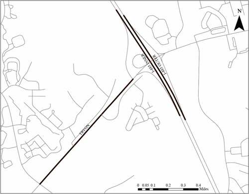
Initially, 1,133 links in an urban area (Mecklenburg County) and 151 links in a rural area (Iredell County) in North Carolina, USA, were considered for this research. These links have uniform geometric, control, and traffic characteristics and include freeway, highway, arterial, collector, and local road links with different posted speed limits and reference speeds.

Data Collection

The raw unprocessed travel time data for both the study areas were gathered from the National Performance Management Research Data Set (NPMRDS) from 1 January 2017 to 31 December 2017 (one year). NPMRDS is a vehicle probe-based and cellphone-based travel time dataset acquired by the Federal Highway Administration (FHWA) to support freight performance measures and urban congestion report programs. This is one of the best data sources currently available to state and metropolitan planning organizations (MPOs) to meet their Moving Ahead for Progress in the 21^st Century Act (MAP-21) and Fixing America’s Surface Transportation (FAST) Act requirements.

For each link, NPMRDS has a unique identification code (traffic message channel, TMC), measurement stamp (date and time of collection), reference speed, travel time of passenger cars only, travel time of trucks only, travel time of all vehicles, and data density at 5-minute intervals. It should be noted that travel time data are collected and archived separately (as three separate data fields) for passenger cars, trucks, and traffic stream (all vehicles). Individual vehicle type details are not available.

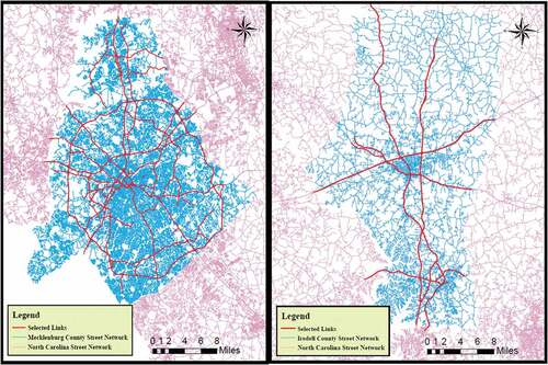
The links with null values and length less than 330 feet (as they may have nearly equivalent travel times for all vehicles while also influencing the values when converted to travel times per unit distance) were excluded from the analysis for each area type. Overall, of the 1,133 links, the unprocessed raw travel time data for passenger cars only and traffic stream was gathered for 894 links while the unprocessed raw travel time data for trucks was gathered for only 798 links in Mecklenburg County. Likewise, of the 151 links, the unprocessed raw travel time data for passenger cars only and traffic stream was gathered for 137 links while the unprocessed raw travel time data for trucks was gathered for only 133 links in Iredell County. Figure 2 shows the study area and selected geographically distributed links in Mecklenburg County and Iredell County. While increasing efforts are being spent by private data sources to collect truck travel time data for higher number of links every year, the difference in the number of links with travel time data for passenger cars only, traffic stream, and trucks is because travel time data specific to trucks were not available for some links in the selected study areas during the study year.

Figure 2. Selected links in Mecklenburg County and Iredell County.

Data Processing and Data Segregation

The raw travel time data was processed using Microsoft Structured Query Language (SQL) Server, MS Excel, and ArcGIS software. The database for each area type were then segregated based on data density to generate a separate dataset for each data density (A, B, and C). In the raw travel time data, data density A indicates the presence of 1 to 4 vehicles, data density B indicates the presence of 5 to 9 vehicles, and data density C indicates the presence of 10 or more vehicles. The data density is considered as an indicator of traffic volume and its composition, i.e. traffic conditions at the time of data collection. It is assumed that data for a greater number of vehicles would be captured if traffic volumes are high or vice versa. The actual number of vehicles present at the time data was collected is not available.

The dataset for each area type and data density were then segregated by DOW, TOD, and reference speed. DOW was classified as Wednesday representing a weekday and Saturday representing a weekend day. Based on traffic patterns in the study areas, TOD was classified as the morning peak period (8 AM – 9 AM), afternoon period (12 PM – 1 PM), evening peak period (5 PM – 6 PM), and night-time period (8 PM – 9 PM). The reference speed from the NPMRDS was categorized into four groups: ≤30 mph, >30 & ≤40 mph, >40 & ≤50 mph, and >50 mph. It is an indicator of the free-flow condition or free-flow speed of the road segment in miles per hour. It is used in this research as a factor influenced by road geometry and posted speed limit.

SQL queries were written to compute the average travel time (ATT) of trucks, the ATT of passenger cars and the ATT of traffic stream for each link, by DOW, TOD, and data density condition. As an example, the ATT of trucks for a link during the morning peak period on a weekday when data density condition is A was computed by summing all available truck travel times, for the link, from 8 AM to 9 AM on Wednesday in data density condition A and dividing with the number of truck travel times used for summation. The same process was used to compute the ATT of passenger cars and the ATT of traffic stream. The ATT values were converted to ATT per mile by dividing with the link length to eliminate inconsistency due to different link lengths.

The ATT (of trucks, passenger cars, and traffic stream) by area type, DOW, TOD, reference speed, and data density for each link are from at least 30 travel time records for each segregated dataset. The ATTs and associated explanatory variables for each link are considered as a separate data sample for analysis and modeling.

Table 1 summarizes the number of data samples for modeling by reference speed, DOW, and TOD. A total of 7,645 data samples were considered for the analysis and development of GEE models. Of these, 5,633 (73.7%) are urban area related data samples while 2,012 (26.3%) are rural area-related data samples. The total data samples are evenly distributed by DOW. The number of data samples for the morning peak period, afternoon period, evening peak period, and night-time period are 1,934 (25.3%), 2,193 (28.7%), 2,022 (26.4%), and 1,496 (19.6%), respectively. Likewise, 5,156 (67.4%), 2,240 (29.3%), and 249 (3.3%) data samples are related to data density A, data density B, and data density C, respectively.

Table 1. Data Samples for GEE Modeling by Reference Speed, DOW, and TOD

DOW	≤ 30 mph	> 30 & ≤ 40 mph	> 40 & ≤ 50 mph	> 50 mph	Total
	Weekday
Morning peak period	74	104	112	671	961
Afternoon period	283	110	118	571	1,082
Evening peak period	140	83	83	689	995
Night-time period	124	90	84	478	776
	Weekend
Morning peak period	68	115	93	697	973
Afternoon period	229	129	96	657	1,111
Evening peak period	175	100	84	668	1,027
Night-time period	143	66	80	431	720
Total	1,236	797	750	4,862	7,645

Generalized Estimating Equation (GEE) Models

Many explanatory variables like the area type, TOD, DOW, posted speed limit, reference speed, traffic volume and composition, and geometric conditions like the number of lanes, shoulder width, radius of curvature, and grade of a link have an effect on truck travel time of the link. As stated previously, the geometric conditions like the number of lanes, lane width, shoulder width, radius of curvature, and grade influence the free-flow condition (free-flow speed and free-flow travel time). Data elements other than the number of lanes are not readily available for each link considered in this research. The number of lanes and traffic volume have a relatively low association with the ATT of trucks (Duvvuri & Pulugurtha, 2021).

GEE models were preferred over ordinary least squares (OLS), analysis of variance (ANOVA), or mixed models to estimate the ATT of trucks to the ATT of passenger cars or traffic stream ratio by negating the effect of missing data elements and exploring correlated, clustered, and non-normal data. In other words, the ATT of trucks and ATT of passenger cars or traffic stream were compared (pairwise) for each link by DOW, TOD, and traffic condition when developing the GEE models. It should be noted that the traffic volume and composition (considered using data density), the lane width, shoulder width, radius of curvature, and grade (considered using the reference speed) are same for the link during the compared DOW and TOD.

Overall, the area type, DOW, TOD, reference speed, and data density were considered as the explanatory variables for developing the GEE models. The DOW and area type were considered as dichotomous variables; weekday as ‘1’ and weekend as ‘0ʹand the urban area as ‘1’ and the rural area as ‘0’. The TOD (morning peak period, afternoon period, evening peak period, and night-time period), data density (data density A, data density B, and data density C), and reference speed group (≤30 mph, >30 & ≤40 mph, >40 & ≤50 mph, and >50 mph) were considered as explanatory variables with night-time period, data density C, and reference speed >50 mph as the respective reference categories (as ‘0’).

The ATT of trucks to the ATT of passenger cars ratio as well as the ATT of trucks to the ATT of traffic stream ratio were explored as the dependent variables. Different types of GEE models can be developed based on the available dataset and data distribution. They include linear, gamma with log-link, Poisson with log-link, and negative binomial with log-link distributions.

As GEE uses the quasi-likelihood method, the Quasi-likelihood under independence criterion, QIC and the corrected version of the quasi-likelihood criterion, QICC were considered as the goodness-of-fit statistics. The value of QIC and QICC should be as low as possible for the best-fitted model. Also, the difference between the QIC and QICC should be as low as possible.

Model Validation

The reliability and feasibility of the developed GEE models were validated using the mean absolute percentage error (MAPE) and root mean square error (RMSE). MAPE is a relative error measure while RMSE is an absolute error measure (Bauer & Tulic, 2018; Jenelius & Koutsopoulos, 2017; Lewis, 1982). They are mathematically represented as in Equation (1)(1) $\text{MAPE}=\frac{1}{\text{n}}{\displaystyle \sum _{\text{t}=1}^{\text{n}}\frac{\left|{\text{Actual}}_{\text{ATT}}-{\text{Predicted}}_{\text{ATT}}\right|}{{\text{Actual}}_{\text{ATT}}}}\times 100$(1) and Equation (2)(2) $\text{RMSE}=\sqrt{\frac{{\displaystyle {\sum }_{\text{t}=1}^{\text{n}}{\left({\text{Actual}}_{\text{ATT}}-{\text{Predicted}}_{\text{ATT}}\right)}^2}}{\text{n}}}$(2) . Eighty percent of the final dataset was used for model development/calibration, while 20% of the final dataset was randomly selected to validate the models. In other words, the randomly selected validation dataset was not used in the model development/calibration.

(1) $\text{MAPE}=\frac{1}{\text{n}}{\displaystyle \sum _{\text{t}=1}^{\text{n}}\frac{\left|{\text{Actual}}_{\text{ATT}}-{\text{Predicted}}_{\text{ATT}}\right|}{{\text{Actual}}_{\text{ATT}}}}\times 100$(1)

(2) $\text{RMSE}=\sqrt{\frac{{\displaystyle {\sum }_{\text{t}=1}^{\text{n}}{\left({\text{Actual}}_{\text{ATT}}-{\text{Predicted}}_{\text{ATT}}\right)}^2}}{\text{n}}}$(2)

where n = the number of observations, Actual_ATT = the observed ATT, and, Predicted_ATT = the predicted ATT.

The lower the MAPE and RMSE, the higher the predictability or accuracy of a model. Per Lewis (Lewis, 1982), a MAPE value under 10% is a highly accurate estimated value; 11–20% is a good estimated value; 21–50% is a reasonable and acceptable estimated value; and >51% is an inaccurate estimated value. Unlike MAPE, RMSE is in relation to the value being estimated and cannot be compared across data at different scales (for example, 0.15 if ATT is expressed in minutes but 9 if ATT is expressed in seconds). In this research, MAPE < 10% and RMSE < 0.15 were considered as criteria to define a valid good model.

RESULTS

The model development was preceded by computing descriptive statistics such as the minimum, the maximum, the mean, and the standard deviation of the ATT of trucks, the ATT of passenger cars, and the ATT of traffic stream. The descriptive statistics showed that the ATT of trucks varied from 0.87 to 9.83 minutes/mile with a mean of 1.46 minutes/mile and 1.26 minutes/mile for urban and rural areas, respectively. The standard deviation of ATT of trucks is 0.84 and 0.68 for urban and rural areas, respectively. Similarly, the ATT of passenger cars varied from 0.81 to 10.17 minutes/mile with a mean of 1.69 minutes/mile and 1.32 minutes/mile for urban and rural areas, respectively. The standard deviation of ATT of passenger cars is 0.97 and 0.74 for urban and rural areas, respectively. The ATT of traffic stream varied from 0.84 to 10.17 minutes/mile with a mean of 1.66 minutes/mile and 1.27 minutes/mile for urban and rural areas, respectively. The standard deviation of ATT of traffic stream is 0.96 and 0.69 for urban and rural areas, respectively. The difference between the maximum ATT and the minimum ATT (per unit distance values) and standard deviations are lower for the rural area (Iredell County) when compared to the urban area (Mecklenburg County).

Correlation Analysis

Pearson correlation coefficients were computed to examine the relationship between data density A, data density B, data density C, TOD (morning peak period, afternoon period, evening peak period, and night-time period), DOW (weekday and weekend), area type, and reference speed categories (≤30 mph, >30 & ≤40 mph, >40 & ≤50 mph, and >50 mph). Table 2 summarizes the computed Pearson correlation coefficients between the explanatory variables. No noticeable multicollinearity problems were observed between the explanatory variables. Per these observations and to be able estimate truck travel time of a link irrespective of the area type, DOW, TOD, reference speed, and traffic patterns, all the explanatory variables were considered for GEE model development.

Table 2. Pearson Correlation Coefficient Matrix

Variable	ID	1	2	3	4	5	6	7	8	9	10	11	12	13	14
Data density A	1	1.00
Data density B	2	−0.92	1.00
Data density C	3	−0.26	−0.11	1.00
Morning peak period	4	0.00	0.04	−0.05	1.00
Afternoon period	5	−0.12	0.06	0.17	−0.36	1.00
Evening peak period	6	0.00	0.03	−0.04	−0.34	−0.38	1.00
Night-time period	7	0.18	−0.14	−0.09	−0.28	−0.31	−0.29	1.00
Weekday	8	−0.03	0.02	0.03	0.00	0.00	0.00	0.02	1.00
Weekend	9	0.03	−0.02	−0.02	0.00	0.00	0.00	0.00	−1.00	1.00
Area type	10	0.09	−0.13	0.11	−0.06	0.04	0.00	0.04	0.00	0.00	1.00
≤ 30 mph	11	0.25	−0.23	−0.05	−0.13	0.12	0.00	0.02	0.00	0.00	0.26	1.00
> 30 & ≤ 40 mph	12	0.16	−0.15	−0.03	0.01	0.01	−0.02	0.00	0.00	0.00	0.20	−0.15	1.00
> 40 & ≤ 50 mph	13	0.08	−0.07	0.00	0.01	0.00	−0.03	0.01	0.02	0.00	0.12	−0.14	−0.11	1.00
> 50 mph	14	−0.34	0.32	0.07	0.09	−0.10	0.04	−0.02	0.00	0.00	−0.40	−0.58	−0.45	−0.43	1.00

The results from the GEE models are discussed next.

GEE Models

The explanatory variables with a significance value greater than or equal to 0.05 were considered to have an insignificant affect and eliminated using backward elimination while developing the GEE models.

As stated previously, linear, gamma with log-link, Poisson with log-link, and negative binomial with log-link distributions were considered to develop the GEE models. The QIC and QICC are the lowest for gamma log-link distribution-based models followed by linear models. However, the mean ATT of trucks to ATT of passenger cars ratio and ATT of trucks to ATT of traffic stream ratio are greater than the median ratios. The Kurtosis values are greater than 10 and the Skewness values are greater than 2, indicating that they are highly skewed and not normally distributed. Therefore, gamma log-link distribution-based models are considered as the best-fit models and only discussed in this paper. The gamma log-link distribution-based models to estimate the ratio (R) can be mathematically represented as follows.

(3) $\text{R= }e\text{[}}{\beta }_o+\text{ { }}(\sum {\beta }_i\times {\text{{ }x}\_i}}}^{)]}$(3)

where β_o is the intercept and β_i is the coefficient of significant explanatory variable ‘i’ (area type, data density, TOD, DOW, and reference speed).

The ratio (R) can be multiplied with the ATT of passenger cars (T_pc) or the ATT of traffic stream (T_ts) to estimate the ATT of trucks (T_t).

Explanatory Variables Influencing the Ratio of the ATT of Trucks to the ATT of Passenger Cars

Table 3 summarizes the results from the gamma log-link distribution-based model with the ATT of trucks to the ATT of passenger cars ratio as the dependent variable. It was observed that all the explanatory variables are significant at a 95% confidence level in this gamma log-link distribution-based model.

Table 3. GEE Model – The ATT of Trucks to the ATT of Passenger Cars Ratio

Variable/Parameter	Coeff.	Std. Error	P-value
Intercept	−0.024	0.0063	<0.05
Area type	0.024	0.0028	<0.05
Data density A	0.052	0.0051	<0.05
Data density B	0.022	0.0046	<0.05
Morning peak period	0.029	0.0037	<0.05
Afternoon period	0.023	0.0037	<0.05
Evening peak period	0.043	0.0042	<0.05
Weekday	−0.007	0.0028	<0.05
≤ 30 mph	0.074	0.0055	<0.05
> 30 & ≤ 40 mph	0.046	0.0059	<0.05
> 40 mph & ≤ 50 mph	0.016	0.0048	<0.05
QIC	82.191
QICC	75.239
RMSE	0.11
MAPE	6%

The results indicate that the minimum ATT of trucks to the ATT of passenger cars ratio is {exp (−0.024)} = 0.976 on a link in a rural area with reference speed >50 mph and data density is C on a weekend day during night-time period. This may sound counterintuitive but not totally unrealistic. Field observations and anecdotal evidence indicate that some trucks drivers drive faster than other vehicles on high speed and low traffic volume roads in rural areas of North Carolina, USA. The mass of trucks and gravity on downgrades in rural areas may also have a catalytic effect on their speeds.

The ratio is higher for a link in an urban area if all the other variables are kept constant. This could be attributed to higher traffic volumes and associated congestion on roads in an urban area.

The ratio is higher for data density A and data density B if all the other variables are kept constant. The results also indicate that the ratio is higher during the morning peak period, afternoon period, and evening peak period when compared to the night-time period. This could be attributed to higher traffic volumes and relative inability of trucks to maneuver or find adequate gaps to overtake during these periods. However, the ratio is marginally lower on a weekday when compared to on a weekend day if all the other variables were kept constant. This could be attributed to higher traffic volumes, associated congestion, and relative inability of vehicles to maneuver or find adequate gaps to overtake on weekdays compared to weekends. The ratio is higher on a link with reference speed ≤50 mph if all the other variables are kept constant, possibly due to design standards and geometric conditions of low-speed roads.

Overall, the coefficients indicate that area type, DOW, TOD, and reference speed influence truck travel times and their effect on surrounding vehicles. From Table 3, the maximum ATT of trucks to the ATT of passenger cars ratio is 1.18 on a link in an urban area with reference speed ≤30 mph and data density is A on a weekday during evening peak period. This implies that ATT of trucks could be as high as 1.18 times the ATT of passenger cars.

Explanatory Variables Influencing the ATT of Trucks to the ATT of Traffic Stream Ratio

Table 4 summarizes the results from the gamma log-link distribution-based model with the ratio of the ATT of trucks to the ATT of all vehicles as the dependent variable. Both, area type and weekday were observed to have an insignificant effect and removed through the backward elimination process.

Table 4. GEE Model – The ATT of Trucks to the ATT of Traffic Stream Ratio

Variable/Parameter	Coeff.	Std. Error	P-value
Intercept	−0.057	0.005	<0.05
Data density A	0.054	0.004	<0.05
Data density B	0.019	0.003	<0.05
Morning peak period	0.039	0.003	<0.05
Afternoon period	0.027	0.003	<0.05
Evening peak period	0.046	0.004	<0.05
≤ 30 mph	0.080	0.005	<0.05
> 30 & ≤ 40 mph	0.054	0.006	<0.05
> 40 mph & ≤ 50 mph	0.015	0.005	<0.05
QIC	73.187
QICC	69.702
RMSE	0.11
MAPE	6%

The results indicate that the ATT of trucks to the ATT of traffic stream ratio is {exp (−0.057)} = 0.945 on a link with reference speed >50 mph, during night-time period and data density is C in a rural area. This is lower than the estimated ATT of trucks to the ATT of passenger cars ratio on a link in a rural area with reference speed >50 mph and data density is C on a weekend day during night-time period. It can be attributed to the lower ATT of passenger cars than the ATT of traffic stream.

The ATT of trucks to the ATT of traffic stream ratio is higher if data density is A or data density is B when compared to data density C, if all the other variables are kept constant. The results also indicate that the ratio is higher during the morning peak period, afternoon period, and evening peak period if all the other variables are kept constant. As stated previously, this could be attributed to higher traffic volumes and relative inability of trucks to maneuver or find adequate gaps to overtake during these periods. Further, the ratio is higher on a link with reference speed ≤50 mph, possibly due to design standards and geometric conditions of low-speed roads.

From Table 4, the maximum ATT of trucks to the ATT of traffic stream ratio is 1.13 on a link with reference speed ≤30 mph and data density is A during evening peak period. This implies that ATT of trucks could be as high as 1.13 times the ATT of traffic stream.

SUMMARY AND DISCUSSION

The concept of PCE has been introduced to account for the effect of trucks on the transportation system performance. Density, speed, headway, volume-to-capacity ratio, and delay were used to assess PCE in the past (Transportation Research Board, 2000; Kockelman & Shabih, 2000; Anwaar et al., 2011; Transportation Research Board, 2010; Transportation Research Board, 2016; Elefteriadou et al., 1995; Geistefeldt, 2009; Huber, 1982; Demarchi & Setti, 2003). The average speed is used to assess the performance of arterial streets and two-lane rural roads, while the general research trends indicate exploring and considering the average speed or travel time-based measures in the future (Mane & Pulugurtha, 2020; Pulugurtha et al., 2020; Rakha et al., 2010; Tu et al., 2007; Van Lint & van Zuylen, 2005; Yang & Wu, 2016). Further, with increasingly available continuous travel time and/or speed data, this research focuses on the effect of trucks compared to passenger cars or traffic stream on the transportation system from a travel time perspective.

The gamma log-link distribution-based models are the best-fitted models with lower QIC and QICC values. The RMSE and MAPE were lower than the considered criteria and are the same for both the gamma log-link distribution-based models.

The results from the gamma log-link distribution-based models indicate that all the explanatory variables except weekday are positively associated with the ATT of trucks to the ATT of passenger cars ratio. However, area type and DOW were insignificant at a 95% confidence level when the ATT of trucks to the ATT of traffic stream was considered as the dependent variable.

The effect is highest during the evening peak period followed by the morning peak period when examined by TOD. On the links with the reference speed ≤50 mph, the ATT of trucks to the ATT of passenger cars ratio and the ATT of trucks to the ATT of traffic stream ratio is higher when compared to the corresponding ratio for links with reference speed >50 mph. The effect is highest for links with reference speed ≤30 mph. Such links are either on lower functional class roads or with geometry conditions like horizontal curves and vertical curves.

The coefficients for data density B, >30 & ≤ 40 mph, and >40 & ≤50 mph are higher when the ATT of trucks to the ATT of passenger cars ratio is the dependent variable than when the ATT of trucks to the ATT of traffic stream ratio is the dependent variable. Contrarily, the coefficients of data density A, morning peak period, afternoon period and evening peak period, and ≤30 mph are higher when the ATT of trucks to the ATT of traffic stream ratio is the dependent variable than when the ATT of trucks to the ATT of passenger cars ratio is the dependent variable. This indicates that vehicle type used for comparison will have a bearing on the results and outcomes.

As was observed by Tu et al. (Tu et al., 2007), the presence of trucks has an influence on the ATT of passenger cars and other vehicles. The findings from past studies (Pulugurtha et al.2020; Pulugurtha & Koilada, 2020; Van Lint & van Zuylen, 2005) indicate that area type, DOW, TOD, and speed limit or reference speed influence traffic stream travel times and related relationships. The findings from this research also indicate a similar influence on truck travel times. Further, the influence of traffic condition, reference speed, DOW, and TOD on the ATT of trucks seem to vary with the area type. It should be noted that the rural area has fundamentally different characteristics with regard to traffic volume, road geometry, intersections, and speed.

CONCLUSIONS

A methodology was proposed and used to examine the relationships and estimate the ATT of trucks to the ATT of passenger cars or traffic stream ratio. The area type was observed to influence the ATT of trucks to the ATT of passenger cars or traffic stream ratio differently. This indicates the need to incorporate the area type as a variable when accounting for the effect of heavy vehicles from a travel time perspective. Similarly, notable differences in the coefficients of other explanatory variables were observed when the ATT of trucks was compared with the ATT of passenger cars and traffic stream for modeling. Overall, the ATT of trucks could be as high as 1.18 times the ATT of passenger cars or as high as 1.13 times the ATT of traffic stream for a link.

The models developed from this research could be transferred and used for urban areas and rural areas similar in size, demographics, topography, and land use patterns as Mecklenburg County and Iredell County in North Carolina, USA. However, it is recommended that the methodology be adopted to develop region-specific models to estimate truck travel time, compare with findings from this research, and proactively use it to plan, design, and manage transportation facilities.

The ATT of trucks could be sometimes lower than the ATT of passenger cars or traffic stream. While this may sound counter-intuitive, anecdotal evidences and field observations indicate that some truck drivers drive faster than other vehicle drivers on high speed low traffic volume roads. The mass of the truck and gravity could also influence the speed of trucks on downgrades, particularly in rural areas, when compared to other vehicles. Though the effects were negated considering ratio of travel times, data density, and reference speed in this research, capturing data, generating separate datasets, and examining the travel time relationships for level sections and on horizontal curves, upgrades, and downgrades by length and surface-type merits an investigation.

Practitioners and road users value travel time. The state, regional, and local agencies determine the operational performance of the road using the level of service (LOS) concept. However, LOS does not directly capture the variability in travel time by vehicle type. Exploring the PCE of trucks and the influence on LOS by geometric and traffic condition from a travel time perspective merits further investigation.

The influence of driver behavior such as speeding, aggressive driving, distracted driving, and drowsy driving on truck travel times should also be further explored in future research. Land use is the dominant variable controlling goods movement patterns (Crowley et al., 1975). The socio-economic characteristics and demographic characteristics, in addition to land use characteristics, within the vicinity of a road link could also be captured and explored as surrogates in future research. Developing truck travel time models using the aforementioned variables will not only help assess their effect but also estimate truck travel time of a link when passenger car or all vehicle travel time are not available.

Travel time data with vehicle type details and the actual number of probe vehicles (used to define data density) was not available for this research. Likewise, light trucks may be used for freight transportation and may have relatively lower but similar effects as large trucks on transportation system performance. Capturing the vehicle type data (e.g., each type of passenger car, light truck, large truck, and bus), the number of probe vehicles, and exploring random effects models or elasticity-based models or machine learning techniques to understand the relationships and/or estimate truck travel time merits further investigation.

Disclaimer

This paper is disseminated in the interest of information exchange. The views, opinions, findings, and conclusions reflected in this paper are the responsibility of the authors only and do not represent the official policy or position of USDOT, NCDOT, the University of North Carolina at Charlotte or other entity. The authors are responsible for the facts and the accuracy of the data presented herein. This paper does not constitute a standard, specification, or regulation.

Acknowledgments

The authors thank the staff of North Carolina Department of Transportation (NCDOT) and Regional Integrated Transportation Information System (RITIS) for their help with data needed for this research. The National Performance Management Research data set used in this research is based upon work supported by the Federal Highway Administration under contract number DTFH61-17-C-00003.

Disclosure statement

No potential conflict of interest was reported by the author(s).

Additional information

Funding

This work was based on ideas and information collected for a project supported by the United States Department of Transportation - Office of the Assistant Secretary for Research and Technology (USDOT/OST-R) University Transportation Centers Program (Grant # 69A3551747127).

References

- Al-Kaisy, A., Jung, Y., & Rakha, H. (2005). Developing passenger car equivalency factors for heavy vehicles during congestion. Journal of Transportation Engineering, 131(7), 514–523. https://doi.org/10.1061/(ASCE)0733-947X(2005)131:7(514)
- Anwaar, A., Van Boxel, D., Volovski, M., Anastasopoulos, P. C., Labi, S., & Sinha, K. C. (2011). Using lagging headways to estimate passenger car equivalents on basic freeway sections. Journal of Transportation of the Institute of Transportation Engineers, 2(1), 5–17.
- Bauer, D., & Tulic, M. (2018). Travel time predictions: Should one model speeds or travel times? European Transport Research Review, 10(2), 46. https://doi.org/10.1186/s12544-018-0315-7
- Bureau of Transportation Statistics. North American Freight Numbers. 2017, https://www.bts.gov/newsroom/2017-north-american-freight-numbers, accessed May 1, 2019
- Bureau of Transportation Statistics. Freight Facts and Figures 2015. 2015, https://www.bts.gov/archive/data_and_statistics/by_subject/freight/freight_facts_2015, accessed May 1, 2019
- Crowley, K. W., Habib, P., Loebl, S., & Pignataro, L. J. (1975). Facilitation of Urban Goods Movement, Mobility of People and Goods in Urban Environment. United States Department of Transportation.
- Demarchi, S., & Setti, J. (2003). Limitations of passenger-car equivalent derivation for all vehicles with more than one truck type. Transportation Research Record: Journal of the Transportation Research Board, 1852(1), 96–104. https://doi.org/10.3141/1852-13
- Dowling, R., List, G., Yang, B., Witzke, E., & Flannery, A. Incorporating Truck Analysis into the Highway Capacity Manual. 2014, TRB, The National Academies Press. https://www.nap.edu/read/22311/chapter/1, accessed May 1, 2019
- Duddu, V. R., Pulugurtha, S. S., & Penmetsa, P. (2018). Illustrating the monetary impact of transportation projects/alternatives using the values of travel time and travel time reliability. Transportation Research Record: Journal of the Transportation Research Board, 2672(51), 88–98. https://doi.org/10.1177/0361198118790378
- Duvvuri, S., & Pulugurtha, S. S. (2021). Truck travel time performance measures and their association with on- and off-network characteristics. Transportation Research Interdisciplinary Perspectives, 12, 100500. https://doi.org/10.1016/j.trip.2021.100500
- Elefteriadou, L., Roess, R. P., & McShane, W. R. (1995). Probabilistic nature of breakdown at freeway merge junctions. Transportation Research Record: Journal of the Transportation Research Board, 1484, 80–89. http://onlinepubs.trb.org/Onlinepubs/trr/1995/1484/1484-011.pdf
- Federal Highway Administration. Commercial Vehicle Size and Weight Program. 2018, https://ops.fhwa.dot.gov/freight/sw/overview/index.htm, accessed August 4, 2021
- FHWA. Federal Motor Carrier Safety Regulations. 2005, https://www.fmcsa.dot.gov/safety/data-and-statistics/motor-carrier-safety-progress-report-september-30-2005, last accessed May 1, 2019.
- Geistefeldt, J. (2009). Estimation of passenger car equivalents based on capacity variability. Transportation Research Record: Journal of the Transportation Research Board, 2130(1), 1–6. https://doi.org/10.3141/2130-01
- Harwood, D. W., Torbic, D. J., Richard, K. R., Glauz, W. D., & Elefteriadou, L. Review of Truck Characteristics as Factors in Roadway Design. NCHRP Report 505, (TRB: The National Academies Press), 2003, https://nacto.org/docs/usdg/nchrprpt505_harwood.pdf, last accessed August 4, 2021.
- Huber, M. J. (1982). Estimation of passenger-car equivalents of trucks in all vehicles. Transportation Research Board, 869, 60–70. http://onlinepubs.trb.org/onlinepubs/trr/1982/869/869-010.pdf
- Jenelius, E., & Koutsopoulos, H. N. (2017). Urban network travel time prediction based on a probabilistic principal component analysis model of probe data. IEEE Transactions on Intelligent Transportation Systems, 19(2), 436–445. https://doi.org/10.1109/TITS.2017.2703652
- Kockelman, K. M., & Shabih, R. A. (2000). Effect of light-duty trucks on the capacity of signalized intersections. Journal of Transportation Engineering, 126(6), 506–512. https://doi.org/10.1061/(ASCE)0733-947X(2000)126:6(506)
- Kong, D., Guo, X., Yang, B., & Wu, D. (2016). Analyzing the impact of trucks on traffic flow based on an improved cellular automaton model. Discrete Dynamics in Nature and Society, 2016, 1236846. https://doi.org/10.1155/2016/1236846
- Lewis, C. D. (1982). Industrial and Business Forecasting Methods: A Practical Guide to Exponential Smoothing and Curve Fitting. Butterworth-Heinemann.
- Mane, A. S., & Pulugurtha, S. S. (2020). Influence of Proximal Land Use and Network Characteristics on Link Travel Time. Journal of Urban Planning and Development, 146(3), 04020028. https://doi.org/10.1061/(ASCE)UP.1943-5444.0000599
- Mathew, S., & Pulugurtha, S. S. Effect of toll roads on travel time reliability over time. In Transportation Research Board 98th Annual Meeting, Washington, DC (TRB), January 13-17, 2019.
- Polus, A., Craus, J., & Grinberg, I. (1981). Downgrade speed characteristics of heavy vehicles. Journal of Transportation Engineering, 107(2), 143–152. https://doi.org/10.1061/TPEJAN.0000916
- Pulugurtha, S. S., Duddu, V. R., Puvvala, R., Thokala, V. R., & Imran, M. S. Commercial Remote Sensing & Spatial Information (CRS & SI) Technologies Program for Reliable Transportation Systems Planning: Volume 2 - Comparative Evaluation of Travel Time Related Performance Measures. Report No. RITARS-12-H-UNCC-2, Prepared for The United States Department of Transportation, Office of the Assistant Secretary for Research and Technology 2015.
- Pulugurtha, S. S., Duddu, V. R., & Thokala, V. R. Travel time based performance measures: examining inter-relationships and recommendations for analysis. In Transportation Research Board 95th Annual Meeting, Washington, DC (TRB), January 10-14, 2016.
- Pulugurtha, S. S., Duddu, V. R., & Venigalla, M. (2020). Evaluating spatial and temporal effects of planned special events on travel time performance measures. Transportation Research Interdisciplinary Perspectives Journal, 6, 100168. https://doi.org/10.1016/j.trip.2020.100168
- Pulugurtha, S. S., & Koilada, K. (2020). Exploring correlations between travel time based measures by year, day-of-the-week, time-of-the-day, week-of-the-year and the posted speed limit. Urban, Planning and Transport Research Journal. https://doi.org/10.1080/21650020.2020.1845230
- Rakha, H., El-Shawarby, I., & Arafeh, M. (2010). Trip travel-time reliability: issues and proposed solutions. Journal of Intelligent Transportation Systems, 14(4), 232–250. https://doi.org/10.1080/15472450.2010.517477
- Transportation Research Board. (1965). Highway Capacity Manual (HCM) 1965. TRB, National Research Council.
- Transportation Research Board. (1985). Highway Capacity Manual (HCM) 1985. TRB, National Research Council.
- Transportation Research Board. (2000). Highway Capacity Manual (HCM) 2000. TRB, National Research Council.
- Transportation Research Board. (2010). Highway Capacity Manual (HCM) 2010. TRB, National Research Council.
- Transportation Research Board. (2016). Highway Capacity Manual, Sixth Edition: A Guide for Multimodal Mobility Analysis. TRB, National Research Council.
- Tu, H., Van Lint, J. W. C., & Van Zuylen, H. J. (2007). Impact of Traffic Flow on Travel Time Variability of Freeway Corridors. Transportation Research Record: Journal of the Transportation Research Board, 1993(1), 59–66. https://doi.org/10.3141/1993-09
- Van Lint, J. W., & van Zuylen, H. J. (2005). Monitoring and predicting freeway travel time reliability: using width and skew of day-to-day travel time distribution. Transportation Research Record: A Journal of the Transportation Research Board, 1917(1), 54–62. https://doi.org/10.1177/0361198105191700107
- Yang, S., & Wu, Y. J. (2016). Mixture models for fitting freeway travel time distributions and measuring travel time reliability. Transportation Research Record: A Journal of the Transportation Research Board, 2594(1), 95–106. https://doi.org/10.3141/2594-13