A dramatic morphological transformation from a spontaneous, organic street pattern to pre-planned-based order: learning from Baghdad city

ABSTRACT

A city can be characterised as a measurable pattern that comprises streets surrounded by block patterns. These street patterns are largely responsible for connectivity and accessibility, which enable people to move and interact. The study compares four samples in a case study in Baghdad, Iraq. The assets of Baghdad today belong to its historical period as its prevailing organic zigzagged network pattern determine its character. However, urban areas outside the historical zone are constructed according to modern schemes and a modernist ideology. This paper tests the connectivity and accessibility of the street network for four selected neighbourhoods. To achieve this, five indicators were applied, namely: intersection density Id, street density Sd, link to node ratio LNR, internal node connectivity INC and external point connectivity EPC. Following that, a correlation for each street parameter within the selected regions was analysed to identify the main characteristics of each variable in each area. Besides connectivity and accessibility, the paper’s aim is to characterise the historical neighbourhood of Baghdad by comparing it with other chosen areas. This study applies two stages to its case study; the first reviews traditional urban pattern and compares this to the other three examples. The second stage includes the selection of three different samples within the same city, where every sample has several common variables. Adopting a quantitative method, the outcomes revealed variation across the characteristics and parameters of the street pattern within the four chosen neighbourhoods. This finding offer a precise platform and key plan for future urban design strategies and planning methods. The research concluded that a greater understanding of street patterns and parameters could help to improve the built environment and the transformation processes of the urban form, particularly when considering walkability, connectivity, accessibility, and sustainability.

KEYWORDS:

• Street network
• street density Sd
• link to node ratio LNR
• internal node connectivity INC
• street connectivity parameters
• intersection density Id
• external point connectivity EPC

Introduction

During the last few decades, morphological studies have prompted demands to develop different research approaches into the urban form and its ingredients. Specifically, they have called for the consideration of key dependent and independent variables, such as urban life, social interaction versus social distancing, and urban sustainability (Al-Saaidy, 2020a, 2020b, 2020c; Al-Saaidy & Alobaydi, 2021a, 2021b; Monteiro & Pinho, 2021; Roosta et al., 2021). Regardless of their classification (cul-de-sac, connected and main or locally, regionally, and so on), streets work as a coherent platform. This unified network platform also defines the relationship between the public and private realm. A literature review was conducted to address the paper’s aims and provide a holistic outline of different aspects of connectivity and accessibility which could inform future research. A considerable number of scholars have addressed street network and connectivity | accessibility, such as (Al-Akkam, 2011; Al-Saaidy, 2019a; Asami et al., 2001; Hall, 2014; Handy et al., 2003; Hess, 1997; Jacobs, 1993; Jiang et al., 1999; Khder et al., 2016; Kim, 2007; Marshall, 2005; Porta & Romice, 2010a, 2010b; Porta et al., 2006a, 2006b, 2008, 2009, 2014; Remali, 2014; Strano et al., 2013; Su et al., 2019; Zlatkovic et al., 2019).

Open spaces and streets shape the symbiotic relationship between the city’s components and its people. Hashim (Hashim et al., 2014) state that the familiar ordinary function of a street is to facilitate various patterns of movement between places. Hence, the street is an open space that mediates built elements within an urban tissue, including different types of spaces such as pedestrian walkways, roads, seating areas and public amenities (Al-Saaidy & Alobaydi, 2021b). Accessibility and connectivity can be seen as significant characteristics when studying the ability of a street network to shape a walkable environment.

Walkability can be categorized as a dependent factor compared with connectivity and accessibility. These latter two factors represent the physical characteristics of the built environment when considering the street pattern. Moreover, the nature of urban form and its ingredients at different neighbourhood scales – micro, macro, local and global – contribute significantly to the formation of street life. Some scholars correlate walkability and other factors, for instance urban quality and community rights, in order to promote greater equity in walking and improve neighbourhoods’ most urgent infrastructural shortages (Massingue & Oviedo, 2021). Indeed, Shields states that, ‘walkability has emerged as not only a set of indexes and metrics but a normative discourse’ [Shields et al., 2021, abstract].

Also, safe walkability and its impact on quality of life could increase street life through the development of pedestrian-oriented urban environments (Lucchesi et al., 2021). Furthermore, Yang argues that, ‘the lack of an active neighbourhood living environment can impact community health to a great extent. One such impact manifests in walkability, a measure of urban design in connecting places and facilitating physical activity’ [Yang et al., 2021, p 1]. Those developing the built environment should understand walkability by acknowledging the influence of space design on walkable spaces, which can vary significantly between pedestrians with various needs, demands, and purposes (Chan et al., 2021).

Accessibility is another criterion for assessing the urban form; over the last decade it has been acknowledged as one of the most critical principles of urban morphology. Although some studies evaluate different street parameters, others compare accessible networks and urban life. It is necessary to conduct further quantitative studies into both perspectives, which can be validated through a comparison of results. The term accessibility has mainly been adopted in transport literature, which basically requires study at the local and global scale of a city. According to Dalvi, ‘accessibility measures have been used in human geography to describe the growth of towns; the location of facilities and functions; and the juxtaposition of land uses’ [Dalvi, 2021, p 15]. In addition, accessibility has an impact on land use and the development of the urban environment. At the micro and macro level of the neighbourhood, the concept of accessibility requires greater focus to capture the street network’s fine characteristics, although some researchers have studied the relationship between accessibility and travel behaviour within the urban form. This type of research examines the different behavioural approaches that address pedestrian demands (Wachs & Koenig, 2021). The current paper seeks to examine the parameters of the street network by studying the physical characteristics at the micro and macro scales of the selected neighbourhoods.

Connectivity is based on a street network property and the quantity of blocks within an urban area. It relates to the street components, particularly the links and nodes or the length of the street. There are arguably two distinct factors – urban form and function – within micro and macro configurational space. These contribute significantly when drawing the connectivity pattern of a certain urban area. However, the definition of connectivity varies as it depends on the field of study, research approach and variables considered. At the micro and macro level of the urban form, the connectivity of a street network helps to optimize urban life while promoting the quality of the surrounding environment. This is attributed to the interrelationship between the street edge characteristics and street parameters. In a street network, there is a reciprocal relationship between block parameters and the value of connectivity. Nevertheless, the plot pattern could have less effect on the connectivity value where the plot(s) is embedded within a block pattern. Moreover, in their research on streets, density, and the superblock, neighbourhood planning units and street connectivity in Abu Dhabi, Alawadi (Alawadi et al., 2021) concluded that plot density does not affect efficiency. On the contrary, a good network design produces high efficiency regardless of its plot density.

This paper identifies the significant parameters of street patterns and the characteristics that enable connectivity and accessibility; it also considers the walkability of different selected urban areas of Baghdad city. For that reason, the current study adopts five of the street variables: intersection density (Id), street density (Sd), link-node ratio (LNR), internal node connectivity (INC) and external point connectivity (EPC). These parameters are employed separately in the four areas and a comparison is made among these samples. The main research process focuses on four street network patterns, namely: (A) organic, (B) hybrid, (C) paralleled, and (D) loop-grid. The potential walkability in such urban forms relies on the different parameters of the street characteristics (specifically in terms of Id. Sd, LNR, INC and EPC).

The street network links buildings and enables the flow of pedestrians and non-pedestrians. Streets characterise urban space in a more practical than a national sense, where people meet and interact with each other. Thus, the study outlines the indicators and their role in enabling the connectivity and accessibility of an urban context. The of street-intersection analysis value increases when studying and comparing different urban areas. Within the street-intersection, five variables are examined, namely Id. Sd, LNR, INC and EPC. This paper also seeks to comprehend the changes that occurred in the urban configuration of the case study, which shifted from fine-grained activities to pre-determined uses underpinned by a new development policy. The transformation is not only limited to the urban tissue, but also impacts (gradually or promptly) new functions that are experienced in the historical pattern of the old city of Baghdad. The methodology applied in this paper includes quantitative methods and a case study strategy.

Research method and case study

The methods applied to identify and examine different aspects of a city can be varied. For example, according to Sommer (Sommer, 2002), a case study is an in-depth investigation that examines and analyses a certain event or phenomenon through the application of multiple methods and approaches to obtain applicable findings. The scope can entail the investigation of a contemporary phenomenon within a defined boundary between the event and its context (Yin, 2014). For this study, the boundaries of the four samples are marked by a circle with a 400-metre radius. This is based on the frequently cited appropriate walking distance and shows the threshold range of a five-minute walk (Al-Saaidy, 2019b; Al-Saaidy & Alobaydi, 2021a; Aultman-Hall et al., 1997; Mehaffy et al., 2010; Randall & Baetz, 2001; Remali, 2014; Tal & Handy, 2012). The main criterion of the samples is their location in four different regions of Baghdad, and their different street patterns which include the network that simultaneously links them (G.I.S.Department, 2016; R.S.GIS.U, 2017).

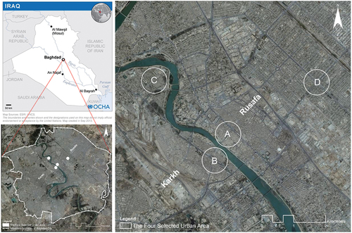
The key objective of the study is to define the traditional area of Baghdad from another perspective by comparing it with other selected neighbourhoods. This research employs two phases in its case study; the first examines the old urban fabric sample and compares this to the other three samples. The second involves the three other samples within the same boundary, where each involves an embedded number of variables that are shared with the other samples. Figure 1 (left) refers to the two fundamental elements of the urban form: human settlements and the Tigris River, and the boundary of the study. Figure 1 (right) shows the border of the four circles, which are drawn with a 400-metre radius to represent the four samples: A organic pattern; B hybrid pattern; C paralleled pattern, and D loop-grid pattern. The paper highlights the street parameters in detail discussing the influential parameters of the street network alongside the attributes that enable connectivity and accessibility, and define the walkability of designated neighbourhoods in Baghdad. In comparison, this paper analyses five street variables: intersection density (Id), street density (Sd), link-node ratio (LNR), internal node connectivity (INC) and external point connectivity (EPC).

Figure 1. (Left) georeferencing satellite imagery of Baghdad city illustrates the boundary of the case study area for the morphological analysis and the urbanism boundary. (right) the four selected urban areas (radius 400 m). Source: drawn by the author based on the georeferencing satellite imagery that authorised by R.S.GIS.U 2017.

Defining street parameters

Intersection density | Id

The intersection density is an indicator to measure the number of intersections per unit of a selected area. It refers to both accessibility and connectivity. A higher number of intersections suggests greater accessibility and connectivity (Cervero & Radisch, 1996; Dill, 2004; Kim, 2007; Reilly & Landis, 2003). Block sizes are inversely associated with the intersection density. The higher the number of street intersections, the smaller the average block in a selected area.

Intersection density I_d can be measured by:

(1) $I_d=N_4+N_3-N_1$(1)

Where I_d is the intersection density, N₄ is the number of four-way nodes or more, N₃ is the number of three-way nodes, and N₁ is the number of cul-de-sacs.

Furthermore, I_d is employed in the centrality analysis of the network by the degree of ‘Integration’ in Space Syntax (Hillier et al., 1976) and ‘Closeness’ in the Multiple Centrality Assessment (MCA) (Porta et al., 2006b). Bourdic (Bourdic et al., 2012) offer another definition to describe the density of the intersection; Cyclomatic refers to the degree of complexity of the street network in terms of the number of links and nodes. Intersection density is weighted differently according to the purpose of the study; for instance, based on the type (four-way, three-way, and one-way) different weights are applied (1, 0, and − 1 respectively). The four-way node has the greatest weight as it is more important, whereas the one-way node has less weight and importance. By using 3 for four-way, 2 for three-way, and 1- for one-way, Remali (Remali, 2014) adopts a different weight for the intersection. In this regard, this research uses the number of nodes and percentages, which are tested in the four-selected areas with a radius of 400-metres, and each type of intersection is named individually. Furthermore, the weighted values respond to the degree of connectivity, accessibility, and permeability, where the four-way I_d (or more) has 2 degrees, three-way has 1 degree, and one-way is equal to − 1. Thus, the formula is:

(2) $I_d=2N_4+1N_3-\hspace{0.17em}1N_1$(2)

The number preceding the letter N is the weight value for each type of intersection. This weight is a relative value when compared with different selected samples that hold the same size, such as the current study.

The node (intersection) is one of the more fundamental urban entities and enables the calculation of the network’s potential accessibility, permeability and connectability. Quantifying nodes in a specific area indicates the street edge length and, in turn, the potential interface between the public and private realm. Increasing the number of links per node maximises the movement-through. In comparison, minimising the number of streets per intersection reduces the flow for both pedestrians and motors (Cervero & Radisch, 1996; Dill, 2004). Bourdic (Bourdic et al., 2012) refer to another indicator that measures the connectivity of the network, namely the Connectivity Index (CI). This measures the mobility of the urban form in terms of connectivity. The higher the CI, the greater the connectivity; thus, a higher number of intersections leads to greater accessibility in the urban fabric.

The formula to measure CI is:

(3) $CI=N_i/A_{total}$(3)

Where CI is the connectivity index, Ni is the number of intersections, and A_total is the total area of the sample. Hence, Bourdic (Bourdic et al., 2012) tend to use the sheer number of intersections regardless of type and without a weighed value. In this study, both indicators are considered: Intersection Density and the Connectivity Index, which are separately addressed for each sample. These are then compared amongst the four samples.

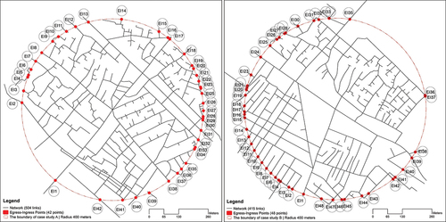
In sample A, the total number of nodes is 387, which includes cul-de-sacs (at 111 nodes), three-way nodes (totaling 249), and four-way nodes (at 27), shown in Figure 2. By employing the I_d equation:

$I_d\hspace{0.17em}|\hspace{0.17em}case\hspace{0.17em}A=2N_4+1N_3-\hspace{0.17em}1N_1\to \left(2\times 27\right)+\left(1\times 249\right)-\left(1\times 111\right)$

$I_d\hspace{0.17em}|\hspace{0.17em}case\hspace{0.17em}A=54+249-111=192$

Figure 2. (Left) sample A, the total number of intersections classified according to the number of links per node: 4 -way nodes, 3-way nodes, and 1 -way nodes (cul-de-sac). (right) case study B (hybrid pattern) that illustrates the number of intersections per type: cul -de-sac, three-way, and four -way node, and the location of the nodes in this sample. Source: drawn by the author based on the georeferencing aerial imagery and base map Baghdad authorised by G.I.S.Department (2016) and R.S.GIS.U (2017).

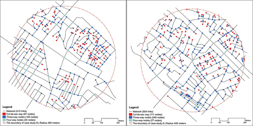
The I_d of sample A is 192. A large number of the intersections are three-way nodes, while four-way nodes are the lowest in number. As cul-de-sacs are dominant links in the oldest part of Baghdad, there are more one-way nodes than any other (Figure 2). Sample B has 314 nodes, as follows: 97 nodes are cul-de-sacs, 183 nodes are three-way intersections, and 34 nodes are four-way intersections (Figure 2). Thus, the value of I_d is:

$I_d\hspace{0.17em}|\hspace{0.17em}sample\hspace{0.17em}B=2N_4+1N_3-\hspace{0.17em}1N_1\to \left(2\times 34\right)+\left(1\times 183\right)-\left(1\times 97\right)$

$I_d\hspace{0.17em}|\hspace{0.17em}sample\hspace{0.17em}B=68+183-97=154$

Like sample A, in sample B the three-way intersections comprise the greater number of nodes; this is followed by cul-de-sacs, and then four-way nodes, which have the fewest intersections.

Sample C includes 70 intersections where the cul-de-sacs total 3, the three-way node 52, and the four-way intersection 15.

The I_d (Intersection Density) for C is:

$I_d\hspace{0.17em}|\hspace{0.17em}sample\hspace{0.17em}C=2N_4+1N_3-\hspace{0.17em}1N_1\to \left(2\times 15\right)+\left(1\times 52\right)-\left(1\times 3\right)$

$I_d\hspace{0.17em}|\hspace{0.17em}sample\hspace{0.17em}C=30+52-3=79$

Sample C exhibits the smallest number of four-way nodes, meaning that the block size is quite large in comparison with samples A and B. This is also the same for the three-way nodes. Also, a lower number of intersections (four-way and three-way) can maximise the block area and consequently minimise the number of blocks (Figure 3). In sample D, there are 62 intersections in total, of which there are 0 cul-de-sac nodes, 54 three-way nodes, and eight four-way nodes.

Figure 3. (Left) case study C : paralleled pattern exhibits the number of intersections for the selected area and their arrangement within the street network. (right) case study D (loop -grid pattern), shows two types of intersection: three -way and four -way node s, while the cul -de -sac disappear s completely. Source: drawn by the author based on the georeferencing aerial imagery and base map Baghdad authori sed by R.S.GIS.U (2017).

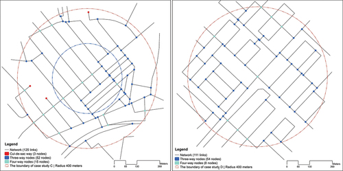
In this regard, the I_d for D is:

$I_d\hspace{0.17em}|\hspace{0.17em}sample\hspace{0.17em}D=2N_4+1N_3-\hspace{0.17em}1N_1\to \left(2\times 8\right)+\left(1\times 54\right)-\left(1\times 0\right)$

$I_d\hspace{0.17em}|\hspace{0.17em}sample\hspace{0.17em}D=16+54-0=70$

Sample D has a lower quantity of intersections overall and the intersection density is the lowest among the four selected areas (Figure 3).

Street density | S_d

Street density is an indicator to measure the number of streets per unit of an area. A higher number refers to more streets and means greater connectivity and accessibility within the network. This indicator has been addressed by a number of scholars; for example, Handy studied urban form and pedestrian choices in six neighbourhoods (Handy, 1996), Crane & Crepeau correlated neighbourhood design and travel behaviour (Crane & Crepeau, 1998), and Matley & Goldman studied pedestrian travel potential in Northern New Jersey (Matley et al., 2000). Dill adopted the indicator to measure network connectivity for bicycling and walking (Dill, 2004), whilst Kim tested the street connectivity of new urbanism projects and their surroundings (Kim, 2007). Tal and Handy measured non-motorised accessibility and connectivity in a robust pedestrian network within nine neighbourhoods in Davis, California (Tal & Handy, 2012). Meanwhile, Bourdic and Salat tested a set of indicators for a new system of cross-scale spatial indicators (Bourdic et al., 2012), and Remali investigated the street density of three types of neighbourhood in the city centre of Tripoli, Libya (Remali, 2014).

Street density is influenced by block characteristics and the number of intersections that influence the development of different patterns, such as one-way, three-way, and four-way nodes. Three formulas to extract the street density per sample are tested: (1) based on street length, (2) by using street area and (3) by considering the total number of streets per chosen sample.

(4) $S_{d1}=S{L}_{total}/A_{total}$(4)

Where S_d is the street density, SL_total is the total length of all streets in the selected sample, and A_total is the total area of the sample.

(5) $S_{d2}=A_{street}/A_{total}\times 100$(5)

Where S_d is street density, A_street is the total area of all streets in the select sample, and A_total is the total area of the sample.

(6) $S_{d3}=N_{street}/A_{total}$(6)

Where S_d is street density, N_street is the total number of streets in the select sample, and A_total is the total area of the sample.

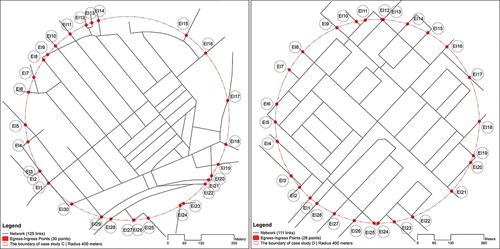
The main concern is for the streets that extend beyond the boundary of the sample. In this regard, the research considers with the real length of the street, meaning that streets that intersect with the border are counted, while the area of the street is subjected to the area of the sample itself. Starting with sample A, the total street length is 18,163.31 metres with a total of 504 links. The entire area of the selected streets in sample A is 122,184.26 m² including squares and parking (Figure 4). This uses the three equations of S_d:

$S_{d1}|\hspace{0.17em}sample\hspace{0.17em}A=18163.31\hspace{0.17em}m\hspace{0.17em}per\hspace{0.17em}502654.82\hspace{0.17em}{m}^2$

$S_{d2}|\hspace{0.17em}sample\hspace{0.17em}A=122184.26\hspace{0.17em}{m}^2/502654.82\hspace{0.17em}{m}^2\times 100=24.31\mathrm{\%}$

$S_{d3}|\hspace{0.17em}sample\hspace{0.17em}A=504\hspace{0.17em}per\hspace{0.17em}502654.82\hspace{0.17em}{m}^2\hspace{0.17em}$

Figure 4. (Left) case study a (organic pattern) which includes 504 links within the selected urban area (502654.82 m 2). (right). Case study B (hybrid pattern) that includes 415 links within the selected urban area (502654.82 m 2). Source: drawn by the author based on the georeferencing aerial imagery and base map baghda d authori sed by G.I.S.Department (2016) and R.S.GIS.U (2017).

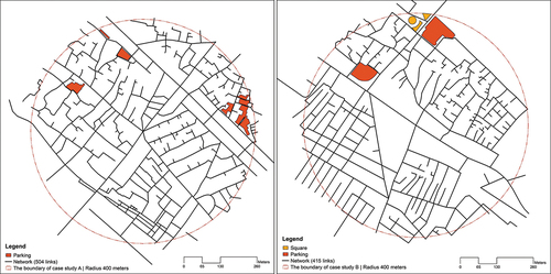
In sample B (Figure 4), within a selected area of approximately 502,654.82 m², there are 415 links and a total length of 17,816.78 metres. The area of the selected streets is 143,075.38 m² which includes squares and parking. The street density for case B is:

$S_{d1}|\hspace{0.17em}sample\hspace{0.17em}B=17816.78\hspace{0.17em}m\hspace{0.17em}per\hspace{0.17em}502654.82\hspace{0.17em}{m}^2$

$S_{d2}|\hspace{0.17em}sample\hspace{0.17em}B=143075.38\hspace{0.17em}{m}^2/502654.82\hspace{0.17em}{m}^2\times 100=28.46\mathrm{\%}$

$S_{d3}|\hspace{0.17em}sample\hspace{0.17em}B=415\hspace{0.17em}per\hspace{0.17em}502654.82\hspace{0.17em}{m}^2$

Sample C consists of 125 streets with a total length of about 12,351.05 metres, and their area is 119,825.13 m². Like all samples, the unified area is 502,654.82 m² (Figure 5). For the street density, the values of S_d are:

$S_{d1}|\hspace{0.17em}sample\hspace{0.17em}C=12351.05\hspace{0.17em}m\hspace{0.17em}per\hspace{0.17em}502654.82\hspace{0.17em}{m}^2$

$S_{d2}|\hspace{0.17em}sample\hspace{0.17em}C=119825.13\hspace{0.17em}{m}^2/502654.82\hspace{0.17em}{m}^2\times 100=23.84\mathrm{\%}$

$S_{d3}|\hspace{0.17em}sample\hspace{0.17em}C=125\hspace{0.17em}per\hspace{0.17em}502654.82\hspace{0.17em}{m}^2$

Figure 5. (Left) case study C (paralleled pattern) consists of 125 links in the selected area (502654.82 m 2). (right) case study D includes 111 links with a total length of about 12,049.69 met res. Source: drawn by the author based on the georeferencing aerial imagery and base map Baghdad authori sed by R.S.GIS.U (2017).

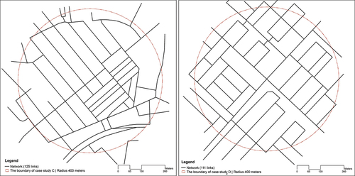
In sample D, there are 111 streets which cover 189,250.17 m2. The entire length is around 120,49.69 metres (Figure 5). The street density is calculated as follows:

$S_{d1}|\hspace{0.17em}sample\hspace{0.17em}D=12049.69\hspace{0.17em}m\hspace{0.17em}per\hspace{0.17em}502654.82\hspace{0.17em}{m}^2$

$S_{d2}|\hspace{0.17em}sample\hspace{0.17em}D=189250.17\hspace{0.17em}{m}^2/502654.82\hspace{0.17em}{m}^2\times 100=37.65\mathrm{\%}$

$S_{d3}|\hspace{0.17em}sample\hspace{0.17em}D=111\hspace{0.17em}per\hspace{0.17em}502654.82\hspace{0.17em}{m}^2$

Link to node ratio | LNR

The Link-Node Ratio is an indicator based on the number of links divided by the number of nodes within the selected area; a higher ratio signifies greater accessibility and connectivity (Figure 6). Through his analysis of pedestrian and transit-friendly features, Ewing Ewing (Ewing, 1999, 1996) referred to the fine-grained pattern of the street network and suggested that this necessitates a simultaneous increase in the number of streets and intersections with short and medium length blocks. Handy (Handy et al., 2003) also refer to the interrelationship between the intersection and street and its influence on connectivity.

Figure 6. Both plans have the same number of nodes. Plan B has two added links, resulting in a link -node ratio of 1.13 versus 0.88 for plan A. Under plan a there is only one route between points a and B. Under plan B there are three potential routes. Source: dill (2004, p 4).

Dill states that the, ‘Link-Node Ratio is an index of connectivity equal to the number of links divided by the number of nodes within a study area. Links are defined as roadway or pathway segments between two nodes. Nodes are intersections or the end of a cul-de-sac’ [49, p 4]. Kim used a link to streets ratio to test the connectivity of streets in five neighbourhoods across the Metro Atlanta region (Kim, 2007). Also, Tal and Handy employed LNR to measure the non-motorised accessibility and connectivity of the network in nine neighbourhoods in the city of Davis, California (Tal & Handy, 2012). Furthermore, Remali’s study on Tripoli, Libya employed the LNR to examine three different street patterns (Remali, 2014).

The formula to measure the LNR is:

(7) $LNR=L_{total}/N_{total}$(7)

Where LNR represents a link to node ratio, L_total is the total number of links in a selected area, and N_total is the total number of nodes (including cul-de-sacs) for the same area.

In the current study, the quantities of links and nodes vary among the four selected areas. After applying LNR, the results exhibit some differences between the two groups of samples (A-B and C-D), where each group includes an approximate value. In sample A, the LNR represents the lowest ratio at about 1.302 with a moderate increase to 1.322 for sample B. The degree of variance between A and B is slight. The LNR trendline for sample C is 1.786 and is highest in sample D at around 1.790. Also, the degree of disparity between samples C and D is minor. The number of cul-de-sacs have a significant role in reducing the number of links and increasing the number of nodes which affects the LNR value for samples A and B. On the other hand, both samples C and D have the lowest number of cul-de-sacs, which means their LNR is higher than samples A and B. Throughout the four samples, the total number of links are higher than the gross quantity of nodes for each single sample: A, B, C, and D (Table 1 and Figure 7).

Figure 7. A chart shows the total number of links and nodes with the link to node ratio (LNR) in the four cases studies. A significant disparity occurs between the two groups, A -B and C -D.

Table 1. The four samples of the case study besides the total number of links and nodes, and the value of the LNR (link to node ratio).

Case Study ID	Total Number of Links	Total Number of Nodes	LNR
Case A	504	387	1.30
Case B	415	314	1.32
Case C	125	70	1.79
Case D	111	62	1.79

The number of streets is essential in combining the LNR to test the network’s connectivity. For example, LNR-case A (1.302) is less than LNR-case D (1.790), although A has the highest number of streets compared with D. Additionally, the one-way node decreases the number of links wherever it is located, such as found in samples A and B, and a little in sample C.

Internal node connectivity | INC

Dill refers to INC, which is also known as the Connected Node Ratio (CNR) or the Connected Intersection Ratio (CIR) (Dill, 2004). All terms have the same meaning in that they evaluate connectivity by dividing the total number of nodes (excepting cul-de-sacs) by the total number of intersections (including cul-de-sacs). A higher value (1.0) indicates that there is no cul-de-sac, and accordingly, the network has greater connectivity.

The formula for the Internal Street Connectivity (INC) is:

(8) $INC=N_{total}-N_{cul}/N_{total}$(8)

Where INC is the internal node connectivity, N_total is the total number of nodes, and N_cul is the total number of cul-de-sacs.

Kim employed the measure to test five different neighbourhoods in the Metro Atlanta region of Georgia, U.S.A. (Kim, 2007). Allen and Song adopted the INC indicator when computing new urbanism with community indicators and the influences of urban evolution management on the urban form (Allen, 1997; Song, 2003). Also, Remali used this indicator when researching three neighbourhoods in the city centre of Tripoli, Libya (Remali, 2014).

By applying the INC formula, the internal node connectivity result for each selected sample is:

$INC\hspace{0.17em}|\hspace{0.17em}sample\hspace{0.17em}A=387-111/387=0.71$

$INC\hspace{0.17em}|\hspace{0.17em}sample\hspace{0.17em}B=314-97/314=0.69$

$INC\hspace{0.17em}|\hspace{0.17em}sample\hspace{0.17em}C=70-3/70=0.96$

$INC\hspace{0.17em}|\hspace{0.17em}sample\hspace{0.17em}D=62-0/62=1.00$

In this study, sample D shows the highest INC value at 1.00, meaning that the number of cul-de-sacs is zero. Meanwhile, the lowest value is for sample B is about 0.69. Sample C is calculated at 0.96, whereas A is about 0.71 representing the smallest value after B. In the oldest area (A), the total number of intersections is higher than for other samples, which total 387 (including 111 cul-de-sacs nodes), and 276 junctions (excluding cul-de-sacs). Therefore, the high number of streets in A increases the connectivity value above the other three samples (B, C, and D). In contrast, D has the maximum INC value at 1.00, but the lowest number of intersections and streets, consequently sample D might be less connected than case A (Table 2 and Figure 8).

Figure 8. The total number of nodes (including and excluding cul -de -sacs) besides the value of the internal node connectivity.

Table 2. The total number of nodes (including and excluding cul-de-sacs) for each case study also, the INC (internal node connectivity).

Case Study ID	Total Number of Nodes	Cul-de-sac	Total Number of Nodes (cul-de-sac excluded)	Internal Node Connectivity INC
Case A	387	111	276	0.71
Case B	314	97	217	0.69
Case C	70	3	67	0.96
Case D	62	0	62	1.00

External point connectivity | EPC

External Node Connectivity (EPC) is an indicator to measure the mean distance between the ingress/egress points located at all intersections and between all streets in the selected area and its boundary (Remali, 2014). The lower the number of ingress/egress points, the longer the distance between these points, and the lower the external connectivity and vice versa. The indicator represents the network’s degree of integration in a selected area within the whole urban context. In this sense, the boundary of the sample can be identified as a nodal border where the number of nodes governs the degree of connectivity and accessibility between a designated part and its surroundings. The indicator was used by Nystuen and Dacey (Nystuen & Dacey, 1961), whilst Song and Knaap employed EPC with several measures of urban form to appraise the progress patterns and trends of single-family residential neighbourhoods in the Portland, Oregon metropolitan area (Song & Knaap, 2004). Betanzo used EPC in his study on density and liveability in three neighbourhoods (Betanzo, 2009), while Remali employed EPC to examine three different patterns of neighbourhood (Remali, 2014).

The EPC equation can be formulated as:

(9) $EPC=L_{total}/P_{total}$(9)

Where EPC is external node connectivity of a selected area, L_total is the total length of the boundary of the sample, and P_total is the total number of ingress/egress points. The total length of the boundary is 2513.27 metres.

The ingress/egress points are mapped onto the boundary of each single sample. Sample A includes 42 points of egress/ingress (Figure 9).

Figure 9. (Left) ingress and egress points of the case study a (organic pattern). (right) ingress and egress points of case study B (hybrid pattern). Source: drawn by the author based on the georeferencing aerial imagery and base map Baghdad authori sed by G.I.S.Department (2016) and R.S.GIS.U (2017).

By using the EPC formula, the level of external connectivity in sample A is:

$EPC\hspace{0.17em}|\hspace{0.17em}sample\hspace{0.17em}A=2513.27/42=59.84\hspace{0.17em}m$

Where the mean distance between the egress/ingress points is 59.84 metres.

In sample B, the total number of ingress/egress points is 48 points, and the value of EPC is:

$EPC\hspace{0.17em}|\hspace{0.17em}sample\hspace{0.17em}B=2513.27/48=52.36\hspace{0.17em}m$

Where the mean distance between the ingress/egress points is 52.36 metres. In sample B, the range between the crossing points is lower than for A, which is due to the different number of ingress/egress points located on the boundary of each sample (Figure 9).

In comparison, 30 ingress/egress points determined the level of external connectivity in sample C (Figure 10). With the total length of the boundary at approximately 2513.27 metres, the EPC for C is:

$EPC\hspace{0.17em}|\hspace{0.17em}sample\hspace{0.17em}C=2513.27/30=83.78\hspace{0.17em}m$

Figure 10. (Left) the total number of ingress/egress points of case study C (paralleled pattern). (right) the total number of ingress/egress points of case study D (loop -grid pattern). Source: drawn by the author based on the georeferencing aerial imagery and base map Baghdad authorised by R.S.GIS.U (2017).

Where the mean distance between the ingress/egress points is 83.78 metres.

The last sample, D, has a boundary encompassing 28 ingress/egress points (Figure 10). Accordingly, the degree of external connectivity is:

$EPC\hspace{0.17em}|\hspace{0.17em}sample\hspace{0.17em}D=2513.27/28=89.76\hspace{0.17em}m$

Where the mean distance between the ingress/egress points is 89.76 metres.

Quantifying the street network: comparison and discussion of the results

Intersection density

It is essential to conduct a comparison across the four samples in terms of Id in order to identify the extent to which the Intersection Density differs from one area to another. Figure 11 illustrates a significant disparity in the number of nodes per type for each sample. It also shows the Id value per case. Sample A has the highest number of one-way nodes (cul-de-sac) at 111 nodes, and D has the lowest at zero. Sample B has the second largest quantity at 97 nodes, while C has only three cul-de-sacs.

Figure 11. The number of nodes per type for each case, and the value of the intersection density per sample. The fluctuation among the four samples is evident; also, the difference between nodes’ quantity is shown per example.

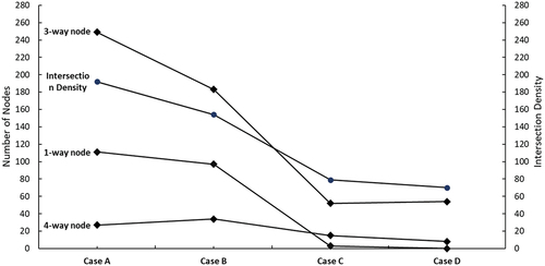
Sample A has the highest number of three-way nodes at 249 nodes, while the other samples are ranked in descending order as B, D, and C whose values are 183, 54, and 52, respectively. Sample B has 34 3- and four-way nodes which is the most among the samples. In contrast, sample D has only eight nodes. The remaining samples, A and C, have 27 and 15 nodes respectively (Figure 11). The Intersection Density (Id) trendline has the highest value at 192 nodes for sample A, and decreases to 70 nodes for D. Moreover, sample B has 154 nodes, and C has 79. The percentage value for each type of node is counted to determine the dominant share per type. The proportion of four-way nodes is highest at 21.43% in sample C and decreases significantly to 6.98% in A. Samples B and D fall between these two extremes at 10.83% and 12.90%, respectively. The percentage of three-way nodes in sample A is 64.34%, and decreases to 58.28% in sample B. However, the percentage is higher in C at 74.29% and D at 87.10%; the latter represents the largest value and contrasts with sample B, which has the lowest percentage (Figure 12).

Figure 12. A graph shows the percentage values for three types of nodes: 4 -way, 3 -way, and one -way node (cul – de -sac) of the four cases A, B, C, and D. Besides, the total number of nodes per sample.

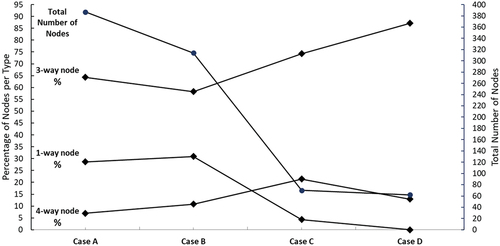
The cul-de-sac trendline shows that the highest percentage is found in for sample B at 30.89%. This significantly decreases for C at 4.29% and 0.00% for D. Meanwhile, sample A has the second largest percentage of one-way nodes at 28.68% (Figure 12). In addition, the total number of nodes per sample fluctuates between two groups, A-B and C-D. In samples A and B, there are 387 and 314 nodes respectively, while this markedly decreases to 70 and 62 nodes for C and D, respectively (Figure 12). Moreover, the three-way node is dominant amongst all samples showing the highest value for each case. The one-way node has second highest value and includes only samples A and B, but not C and D. The number of four-way nodes is lowest in A and B and but highest in samples C and D (Figure 11 and 12). Sample A has the highest number for the Intersection Density (Id, weighted value) and Connectivity Index (CI, non-weighted value). It is followed by sample B with the second most significant value, while samples C and D are ranked third and fourth with the lowest quantities of Id and CI.

Street density

Sample A has the greatest length at 18,163.31 metres. This decreases to 17,816.78 metres for B, and then falls sharply for samples C and D at 12,351.05 and 12,049.69 metres, respectively. Moreover, the total number of streets follows the same trendline as the gross length of streets. In this regard, sample A also has the largest number of streets at 504 links, while D has the lowest at 111 links. Sample B has the second largest at 415 while C has 125 links (Table 3 and Figure 13).

Figure 13. The total length of the selected streets per case study, and the total number of streets. It shows the degree of disparity among the four samples A, B, C, and D.

Table 3. The parameters of the street density extracted from the unified area (502654.82 m²) for the four cases A, B, C, and D.

Case study ID		Street Density Parameters
	Case study area	The total number of streets	The total length of streets	Street area including (parking & squares)	The streets area to case study area ratio %
Case A	502654.82	504	18163.31	122184.26	24.31
Case B	502654.82	415	17816.78	143075.38	28.46
Case C	502654.82	125	12351.05	119825.13	23.84
Case D	502654.82	111	12049.69	189250.17	37.65

Regarding the statistical standards – minimum, median, average, and maximum – the comparison highlights key differences, especially between the two groups A-B and C-D. Sample A has the shortest (minimum) street length at 2.01 metres, which is followed by 3.27, 5.68, and 6.16 for B, D, and C, respectively. In comparison, sample C has the greatest (maximum) street length at about 382.18 metres, while the remaining samples (in descending order) are D, A and B, at 368.53, 233.25 and 227.20 metres, respectively. Furthermore, sample D has the highest value for both the average (108.56) and median (80.83), which contrasts with A which has the lowest average (36.04) and median (28.48). After sample D, C also has a comparatively high average at 98.81 and median at 73.23, while sample B has the second to lowest average (42.93) and median (32.80) (Table 4 and Figure 14).

Figure 14. A chart of statistical standards of the length of the streets in terms of minimum, median, average, and maximum for the four samples A, B, C, and D.

Table 4. Arithmetical standards of the length of the streets about minimum, median, average, and maximum for the four samples A, B, C, and D.

Case study ID		Arithmetical standards of the Streets Length
	Minimum	Median	Average	Maximum
Case A	2.01	28.48	36.04	233.25
Case B	3.27	32.80	42.93	227.20
Case C	6.16	73.23	98.81	382.18
Case D	5.68	80.83	108.56	368.53

Moreover, the other significant assessment is between the length of streets and their total area for each selected area. Although sample A has the greatest gross street length, it has the smallest area for the entire street (except for C). This contrasts with sample D, which has the largest area for the total streets, which contrasts with the lower value for the length of the whole street. Also, sample B reflects the same trend as A, whereas both values are closer to each other for sample C (Figure 15). The oldest area (sample A) is recognised for its narrow street widths, which reduce the total area of the selected streets, although the sample has the highest value for both the full length and number of streets. However, sample D has the lowest total length and number of streets, and the highest amount of street area, as the street dimensions are far wider than those in A (Figure 15).

Figure 15. The comparison between two significant values: the total area of the selected streets and their full length for each case study.

Link to node ratio

A high ratio confirms that the network is connected and permeable, and vice versa. Consequently, samples, A and B have less connectivity while C and D have higher connectivity (Figure 16). Although sample A has the highest number of streets, it also has a large quantity of cul-de-sac streets. This number is lower in samples B and C, and cul-de-sacs disappear completely in D.

Figure 16. Link to node ratio for the four selected samples: a (organic). B (hybrid), C (paralleled), and D (loop – grid pattern).

Internal node connectivity

The maximum amount calculated for this indicator is one, meaning that the network system is free from cul-de-sac streets. Thus, sample D has the highest INC value, which gives it greater connectivity (like C that has a similarly high value) than A and B, which both have a high number of cul-de-sacs (Figure 17).

Figure 17. Internal node connectivity for the four selected samples: a (organic). B (hybrid), C (paralleled), and D (loop -grid pattern).

External point connectivity

Tracking the EPC trendline in Figure 18, shows that sample A has a 59.84 metre mean distance with 42 points ingress/egress points. The line decreases to 52.36 metres for sample B with 48 points (ingress/egress), and then increases substantially to 83.78 metres as a mean distance for sample C, which has 30 ingress/egress points. The highest EPC value is for sample D at about 89.76 metres, which represents the mean distance (Table 5). A high EPC value means substantial spacing between the ingress/egress points and the lowest connectivity between the selected area and its surroundings. Both samples A and B exhibit far lower spacing between their peripheral points.

Figure 18. The external point connectivity value EPC of the four samples A, B, C, and D.

Table 5. The mean EPC distance and the total number of ingress/egress points. The total length of the boundary per case study.

Case Study ID	Total Length of the Boundary	Total Number of Ingress | Egress Points	Mean Distance | EPC
Case A	2513.27	42	59.84
Case B	2513.27	48	52.36
Case C	2513.27	30	83.78
Case D	2513.27	28	89.76

The network for both A and B consists of a significant number of streets (A has 504 links and B has 415 links), which leads to an increasing number of crossing points on the boundary. On the other hand, samples C and D have larger spaces between their ingress/egress points (the EPC is 83.78 metres for C and 89.76 metres for D) as their external connectivity decreases. Furthermore, the network for samples C and D has a smaller number of links (C has 125 links and D has 111 links).

Recently, several scholars have investigated different aspects of connectivity and accessibility, and the term walkability. They have tended to focus on urban form ingredients, meaning they addressed the street, density, and block pattern to determine the efficiency of street networks in certain neighbourhoods. One study, for instance, focused on ‘streets, density, and the superblock: neighborhood planning units and street connectivity in Abu Dhabi’ (Alawadi et al., 2021), and concluded that plot density does not influence efficiency. Instead, a good network design enables great efficiency regardless of its plot density (Alawadi et al., 2021). However, this paper has focused more on the street network and its ingredients, as represented by streets and intersections. Moreover, Al-Saaidy et al. examined street centrality and human density in different urban forms in Baghdad, Iraq (Al-Saaidy & Alobaydi, 2021b). In comparison, this study considered centrality, another element of street patterns, by employing Multiple Centrality Assessment (MCA) to measure betweenness centrality and its correlation to the density of people in a certain street. Thus, this study adopted the metric properties of the street network in order to capture the particular parameters of various street patterns identified as: (A) organic pattern, (B) hybrid pattern, (C) paralleled pattern, and (D) loop-grid pattern.

Conclusion

The paper considered the street network and its parameters (intersection density Id, street density Sd, link to node ratio LNR, internal node connectivity INC and external point connectivity EPC) as one of the ingredients of urban form. Across the four selected neighbourhoods (A organic pattern, B hybrid pattern, C paralleled pattern and D loop-grid pattern), it was found that the traditional part of the city (sample A) exhibits more exceptional values regarding street parameters. The spatial pattern of sample A follows a spontaneous order in the creation of its street network, which could be the most important influence on its form. The bottom-up approach in formulating the street layout in sample A grants a greater diversity of network in terms of quantity and length.

The relationship between the two primary components of the street structure, namely link (street) and node (intersection), were analysed. Five variables were analysed across the four selected urban areas of Baghdad. Each case exhibited distinct values regarding the selected variables (Id, Sd, LNR, INC and EPC). Three fundamental techniques were utilised to present these indicators: georeferencing maps, charts, and tables. The four selected samples yielded different responses to the connectivity value on which network parameters were based. Concerning the intersection density Id, sample A | organic pattern exhibited the highest level of connectivity. This was followed by sample B | hybrid pattern with the second greatest connectivity value. Both samples C | paralleled pattern and D | loop-grid pattern had lower quantities of Id meaning they were less connected. Furthermore, the traditional area in sample A was distinguished by its narrow street widths which reduce the total area of the selected streets, despite the sample had the highest values for the length and number of streets.

Nevertheless, sample D had the lowest total length and number of streets, but the highest amount of street area, although the street dimensions were completely different, and wider than those in case A. This means that a sample with the greatest street area does not necessarily have the highest connectivity. The same concern can be applied to the link to node ratio, as both samples C and D have the highest value of LNR and thus the highest connectivity. Both samples include the lowest number of streets compared with A and B. This consideration is different in the two neighbourhoods, A and B, which had the largest quantities of streets and the lowest LNR values.

Accessibility and connectivity closely relate to INC (Internal Node Connectivity) in terms of the number of cul-de-sacs per area; thus a higher number of cul-de-sacs means less network accessibility, and vice versa. This phenomenon was evident between samples A (traditional area) and D (modern pattern). The former had the highest number of cul-de-sacs while the latter had none. However, neighbourhood D is more accessible than sample A, as demonstrated by the INC. Across the four chosen areas, samples A and B contained the highest external point connectivity (EPC) for ingress and egress, which meant greater connectivity and accessibility to and from the surrounding area. This characteristic is more limited in both C and D, which have modest amounts of external points. Controlling the connectivity and accessibility of the street network is not limited to one factor or indicator but also requires the testing of a set of parameters in order to determine different aspects of connectivity and accessibility in a certain area. This consideration is evident when comparing the traditional area represented by sample A and the other neighbourhoods.

Thus, different street patterns affect the overall pattern of a city in terms of accessibility and connectivity. A city comprises different network patterns that present particular challenges when considering accessibility and connectivity. Thus, when studying a city, the priority would be to determine accessibility and connectivity, which would consider different key concepts, such as urban life, social interaction, and a 15-minute city. Also, future research could consider how block parameters affect connectivity and accessibility, and the correlation between pedestrian flow and street parameters (plot | block). Moreover, this study revealed the need to study comparative approaches among traditional street patterns and/or modern street patterns within various urban areas – across one city, different cities, and various countries. This could help to build a valuable database of the characteristics and parameters of street patterns. The forthcoming paper will study three parameters within the same case study, and focus on the configuration of the street pattern: grid pattern ratio GPR, pedestrian route directness factor |PRD/PRF, ped-shed and effective walking area |PS and EWA.

Disclosure statement

No potential conflict of interest was reported by the author.

References

- Al-Akkam, A. J. (2011). Urban characteristics: The classification of commercial street in Baghdad city. Emirates Journal for Engineering Research, 16(2), 49–26.
- Alawadi, K., Hong Nguyen, N., Alrubaei, E., & Scoppa, M. (2021). Streets, density, and the superblock: Neighborhood planning units and street connectivity in Abu Dhabi. Journal of Urbanism: International Research on Placemaking and Urban Sustainability, 16(2), 1–28. https://doi.org/10.1080/17549175.2021.1944281
- Allen, E. Measuring the new urbanism with community indicators. in Contrasts and transitions, American Planning Association National Conference American Planning Association, San Diego, CA. 1997.
- Al-Saaidy, H. J. E. (2019a). Measuring urban form and urban life: Four case studies in Baghdad. University of Strathclyde.
- Al-Saaidy, H. J. E. (2019b). Measuring urban form and urban life: Four case studies in Baghdad, Iraq, in Architecture. University of Strathclyde, Department of Architecture.
- Al-Saaidy, H. J. E. (2020a). Lessons from Baghdad city conformation and essence. In A. Almusaed, A. Almusaed, & L. Truong - Hong (Eds.), Sustainability in urban planning and design (pp. 387–417). IntechOpen. https://doi.org/10.5772/intechopen.88599
- Al-Saaidy, H. J. E. (2020b). Urban form elements and urban Potentiality (literature review). Journal of Engineering, 26(9), 65–82. https://doi.org/10.31026/j.eng.2020.09.05
- Al-Saaidy, H. J. E. (2020c). Urban Morphological Studies (Concepts, Techniques, and Methods). Journal of Engineering, 26(8), 100–111. https://doi.org/10.31026/j.eng.2020.08.08
- Al-Saaidy, H. J. E., & Alobaydi, D. (2021a). Measuring geometric properties of urban blocks in Baghdad: A comparative approach. Ain Shams Engineering Journal, 12(3), 3285–3295. https://doi.org/10.1016/j.asej.2021.04.020
- Al-Saaidy, H. J. E., & Alobaydi, D. (2021b). Studying street centrality and human density in different urban forms in Baghdad, Iraq. Ain Shams Engineering Journal, 12(1), 1111–1121. https://doi.org/10.1016/j.asej.2020.06.008
- Asami, Y., Kubat, A. S., & Istek, C. (2001). Characterization of the street networks in the traditional Turkish urban form. Environment and Planning B: Planning and Design, 28(5), 777–795. https://doi.org/10.1068/b2718
- Aultman-Hall, L., Roorda, M., & Baetz, B. W. (1997). Using GIS for evaluation of neighborhood pedestrian accessibility. Journal of Urban Planning and Development, 123(1), 10–17. (1997)123:1(10). https://doi.org/10.1061/(ASCE)0733-9488(1997)123:1(10)
- Betanzo, D. (2009). Exploring density liveability relationships. The Built & Human Environment Review, 2(1), 23–42.
- Bourdic, L., Salat, S., & Nowacki, C. (2012). Assessing cities: A new system of cross-scale spatial indicators. Building Research & Information, 40(5), 592–605. https://doi.org/10.1080/09613218.2012.703488
- Cervero, R., & Radisch, C. (1996). Travel choices in pedestrian versus automobile oriented neighborhoods. Transport Policy, 3(3), 127–141. https://doi.org/10.1016/0967-070x(96)00016-9
- Chan, E. T., Schwanen, T., & Banister, D. (2021). Towards a multiple-scenario approach for walkability assessment: An empirical application in Shenzhen, China. Sustainable Cities and Society, 71, 102949. https://doi.org/10.1016/j.scs.2021.102949
- Crane, R., & Crepeau, R. (1998). Does neighborhood design influence travel?: A behavioral analysis of travel diary and GIS data. Transportation Research part D. Transportation Research, Part D: Transport & Environment, 3(4), 225–238. https://doi.org/10.1016/S1361-9209(98)00001-7
- Dalvi, M. Q. (2021). Behavioural modelling, accessibility, mobility and need: Concepts and measurement, in Behavioural travel modelling. Routledge.
- Dill, J. Measuring network connectivity for bicycling and walking. in 83rd Annual Meeting of the Transportation Research Board, Washington, DC. 2004.
- Ewing, R. (1999). Pedestrian and transit friendly design: A primer for Smart growth. 1999. International City/County Management Association and Smart Growth Network.
- Ewing, R. H. (1996). Pedestrian and transit friendly design. Florida Department of Transportation: American Planning Association.
- G.I.S.Department. (2016). The traditional area of Baghdad based on Polservice, Geokart, Poland, rectified by Dep. Of GIS, in department of geographic information system GIS, mayoralty of Baghdad. The official letter, No.: O.P.U 420, Date: 24/10/2016 issued by University of Technology, Office of the President.
- Hall, P. M. (2014). Good cities, better lives: How Europe discovered the lost art of urbanism. (F. Nicholas, Ed.). Abingdon.
- Handy, S. (1996). Urban form and pedestrian choices: Study of Austin neighborhoods. Transportation Research Record: Journal of the Transportation Research Board, 1552(1), 135–144. https://doi.org/10.1177/0361198196155200119
- Handy, S., Paterson, R. G., & Butler, K. S. (2003). Planning for street connectivity: Getting from here to there. American Planning Association, Planning Advisory Service.
- Hashim, N., Moirongo, B., & Makworo, M. (2014). The role of urban space design characteristics in influencing social life of Swahili streets: The case of old town Mombasa. Journal of Agriculture Science & Technology, 15(1), 180–191.
- Hess, P. M. (1997). Measures of connectivity [streets: Old paradigm, new investment]. Places, 11(2), 58–65.
- Hillier, B., Leaman, A., Stansall, P., & Bedford, M. (1976). Space syntax. Environment and Planning B: Planning and Design, 3(2), 147–185. https://doi.org/10.1068/b030147
- Jacobs, A. B. (1993). Great streets. MIT Press.
- Jiang, B., Claramunt, C., & Batty, M. (1999). Geometric accessibility and geographic information: Extending desktop GIS to space syntax. computers. Computers, Environment and Urban Systems, 23(2), 127–146. https://doi.org/10.1016/S0198-9715(99)00017-4
- Khder, H. M., Mousavi, S. M., & Khan, T. H. (2016). Impact of street’s physical elements on walkability: A case of Mawlawi street in Sulaymaniyah, Iraq. International Journal of Built Environment and Sustainability, 3(1). https://doi.org/10.11113/ijbes.v3.n1.106
- Kim, J. Testing the street connectivity of new urbanism projects and their surroundings in Metro Atlanta region. in Proceedings, 6th International Space Syntax Symposium, İstanbul, İstanbul, Turkey. 2007.
- Lucchesi, S. T., Larranaga, A. M., Bettella Cybis, H. B., Abreu e Silva, J. A. D., & Arellana, J. A. (2021). Are people willing to pay more to live in a walking environment? A multigroup analysis of the impact of walkability on real estate values and their moderation effects in two global south cities. Research in Transportation Economics, 86, 100976. https://doi.org/10.1016/j.retrec.2020.100976
- Marshall, S. (2005). Streets and patterns. (Dawsonera, Ed). Spon.
- Massingue, S. A., & Oviedo, D. (2021). Walkability and the right to the city: A snapshot critique of pedestrian space in Maputo. Mozambique Research in Transportation Economics, 86, 101049. https://doi.org/10.1016/j.retrec.2021.101049
- Matley, T., Goldman, L., & Fineman, B. (2000). Pedestrian travel potential in Northern new Jersey: A metropolitan Planning organization’s approach to identifying investment priorities. Transportation Research Record: Journal of the Transportation Research Board, 1705(1), 1–8. https://doi.org/10.3141/1705-01
- Mehaffy, M., Porta, S., Rofè, Y., & Salingaros, N. (2010). Urban nuclei and the geometry of streets: The ‘emergent neighborhoods’ model. Urban Design International, 15(1), 22–46. https://doi.org/10.1057/udi.2009.26
- Monteiro, C., & Pinho, P. (2021). Comparing approaches in urban morphology. Journal of Urbanism: International Research on Placemaking and Urban Sustainability, 15(4), 1–28. https://doi.org/10.1080/17549175.2021.1936602
- Nystuen, J. D., & Dacey, M. F. (1961). A graph theory interpretation of nodal regions. Papers in Regional Science, 7(1), 29–42. https://doi.org/10.1111/j.1435-5597.1961.tb01769.x
- Porta, S., Crucitti, P., & Latora, V. (2006a). The network analysis of urban streets: A dual approach. physica A: Statistical mechanics and its applications. Physica A: Statistical Mechanics and Its Applications, 369(2), 853–866. https://doi.org/10.1016/j.physa.2005.12.063
- Porta, S., Crucitti, P., & Latora, V. (2006b). The network analysis of urban streets: A primal approach. Environment & Planning B, Planning & Design, 33(5), 705–725. https://doi.org/10.1068/b32045
- Porta, S., Crucitti, P., & Latora, V. (2008). Multiple centrality assessment in Parma: A network analysis of paths and open spaces. urban design International. Urban Design International, 13(1), 41–50. https://doi.org/10.1057/udi.2008.1
- Porta, S., & Romice, O. (2010a). Analysis brief: Comparative analysis of urban Fabrics. Strathclyde University.
- Porta, S. and Romice, O. (2010b). Plot-based urbanism: Towards time-consciousness in place-making. Working paper. University of Strathclyde, Glasgow. UDSU - Urban Design Studies Unit, University of Strathclyde, Dept. of Architecture. 1–39.
- Porta, S., Romice, O., Maxwell, J. A., Russell, P., & Baird, D. (2014). Alterations in scale: Patterns of change in main street networks across time and space. Urban Studies, 51(16), 3383–3400. https://doi.org/10.1177/0042098013519833
- Porta, S., Strano, E., Iacoviello, V., Messora, R., Latora, V., Cardillo, A., Wang, F., & Scellato, S. (2009). Street centrality and densities of retail and services in Bologna, Italy. Environment and Planning B: Planning and design. Environment & Planning B, Planning & Design, 36(3), 450–465. https://doi.org/10.1068/b34098
- Randall, T. A., & Baetz, B. W. (2001). Evaluating pedestrian connectivity for suburban sustainability. Journal of Urban Planning and Development, 127(1), 1–15. (2001)127:1(1). https://doi.org/10.1061/(ASCE)0733-9488(2001)127:1(1)
- Reilly, M. and Landis, J. (2003). The influence of built-form and land use on mode choice. University of California, Berkeley: University of California Transportation Center Research Paper.
- Remali, A. M. (2014). Capturing the essence of the capital city : Urban form and urban life in the city centre of Tripoli, Libya. In Department of Architecture. United Kingdom: University of Strathclyde.
- Roosta, M., Javadpoor, M., & Ebadi, M. (2021). A study on street network resilience in urban areas by urban network analysis: Comparative study of old, new and middle fabrics in shiraz. International Journal of Urban Sciences, 26(2), 1–23. https://doi.org/10.1080/12265934.2021.1911676
- R.S.GIS.U. (2017). The georeferencing aerial imagery, in remote sensing and GIS unit, building and construction Engineering Department, University of Technology, Baghdad. The official letter, No.: 1578, Date: 01/11/2017.
- Shields, R., Gomes da Silva, E. J., Lima e Lima, T., & Osorio, N. (2021). Walkability: A review of trends. Journal of Urbanism: International Research on Placemaking and Urban Sustainability, 16(1), 1–23. https://doi.org/10.1080/17549175.2021.1936601
- Sommer, R. (2002). A practical guide to behavioral research : Tools and techniques. (S. Barbara Baker, Ed). Oxford University Press.
- Song, Y. (2003). Impacts of urban growth management on urban form: A comparative study of Portland, Oregon, Orange County, Florida and Montgomery County, Maryland. National Center for Smart Growth Research and Education, University of Maryland.
- Song, Y., & Knaap, G.-J. (2004). Measuring urban form: Is Portland winning the war on sprawl? Journal of the American Planning Association, 70(2), 210–225. https://doi.org/10.1080/01944360408976371
- Strano, E., Viana, M., da Fontoura Costa, L., Cardillo, A., Porta, S., & Latora, V. (2013). Urban street networks, a comparative analysis of ten European cities. Environment & Planning B, Planning & Design, 40(6), 1071–1086. https://doi.org/10.1068/b38216
- Su, S., Zhou, H., Xu, M., Ru, H., Wang, W., & Weng, M. (2019). Auditing street walkability and associated social inequalities for planning implications. Journal of Transport Geography, 74, 62–76. https://doi.org/10.1016/j.jtrangeo.2018.11.003
- Tal, G., & Handy, S. (2012). Measuring nonmotorized accessibility and connectivity in a robust pedestrian network. Transportation Research Record: Journal of the Transportation Research Board, 2299(1), 48–56. DOI. https://doi.org/10.3141/2299-06
- Wachs, M., & Koenig, J. G. (2021). Behavioural modelling, accessibility, mobility and travel needs. Edited by: David A. Hensher, Peter R. Stopher. In Behavioural travel modelling (pp. 698–710). Routledge.
- Yang, S., Chen, X., Wang, L., Wu, T., Fei, T., Xiao, Q., Zhang, G., Ning, Y., & Jia, P. (2021). Walkability indices and childhood obesity: A review of epidemiologic evidence. Obesity Reviews, 22(S1), e13096. https://doi.org/10.1111/obr.13096
- Yin, R. K. (2014). Case study research : Design and methods. SAGE.
- Zlatkovic, M., Zlatkovic, S., Sullivan, T., Bjornstad, J., & Kiavash Fayyaz Shahandashti, S. (2019). Assessment of effects of street connectivity on traffic performance and sustainability within communities and neighborhoods through traffic simulation. Sustainable Cities and Society, 46, 101409. https://doi.org/10.1016/j.scs.2018.12.037