Back stress strengthening and strain hardening in gradient structure

Abstract

We report significant back stress strengthening and strain hardening in gradient structured (GS) interstitial-free (IF) steel. Back stress is long-range stress caused by the pileup of geometrically necessary dislocations (GNDs). A simple equation and a procedure are developed to calculate back stress basing on its formation physics from the tensile unloading–reloading hysteresis loop. The gradient structure has mechanical incompatibility due to its grain size gradient. This induces strain gradient, which needs to be accommodated by GNDs. Back stress not only raises the yield strength but also significantly enhances strain hardening to increase the ductility.

Impact Statement: Gradient structure leads to high back stress hardening to increase strength and ductility. A physically sound equation is derived to calculate the back stress from an unloading/reloading hysteresis loop.

GRAPHICAL ABSTRACT

Keywords:

• Back Stress
• Geometrically Necessary Dislocations
• Work Hardening
• Ductility
• Gradient Structure

Gradient structure in metals represents a new strategy for producing a superior combination of high strength and good ductility.[1–6] The gradient structure usually consists of a nanostructured (NS) surface layer with increasing grain size along the depth to reach coarse-grained (CG) sizes in the central layer.[2,4]

Gradient structure can promote ductility significantly,[2,4–9] which is measured under tensile loading. The NS layer in a gradient structure may sustain a large amount of tensile strain,[2,4] because they are constrained by the CG layer. It was reported that the gradient structured (GS) Cu derives its ductility from the confinement of the soft CG core,[2,10] and from strong grain growth in the NS layer by mechanically driven grain growth during tensile deformation. Nanostructures in high-purity copper are known to be unstable at room temperature, and mechanical-driven grain growth in nanocrystalline metals has been extensively reported.[11–16] For GS metals with stable gradient structures, however, their high ductility is attributed to extra strain hardening due to the presence of strain gradient and the change of stress states, which generates geometrically necessary dislocations (GNDs) and promotes the generation and interaction of dislocations.[3,4,17, 18] Furthermore, the gradient structure is observed to produce an intrinsic synergetic strengthening, with its yield strength much higher than that calculated by the rule of mixture from separate gradient layers,[3] which is attributed to the macroscopic stress gradient and plastic incompatibility between layers.[3,4]

The nature of plastic deformation in the gradient structure is still not very clear.[1,2] In fact, the gradient structure can be approximately regarded as the integration of many thin layers with increasing grain sizes.[3,4] The gradient structure deforms heterogeneously due to plastic incompatibilities between neighboring layers with different flow behaviors and stresses under applied strains. As such, it is reasonable to anticipate the development of the strain gradient and internal stresses during plastic deformation, as a result of the plastic incompatibilities between different layers, similar to what happens in composites [19–21] and dual-phase structures.[22]

Back stress has been reported to play a crucial role in strain hardening, strengthening and mechanical properties.[21–23] It is a type of long-range stress exerted by GNDs that are accumulated and piled up against barriers. It interacts with mobile dislocations to affect their slip.[24] The back stress reduces the effective resolved shear stress for dislocation slip because it always acts in the opposite direction of the applied resolved shear stress. In a heterogeneous structure, strain will be inhomogeneous but continuous, producing strain gradients, which needs to be accommodated by GNDs.[23,25–27] It has been observed that back stress strengthening and back stress strain-hardening are primarily responsible for unprecedented combination of strength and ductility of heterogeneous lamella Ti, which was found as strong as ultrafine-grained Ti and as ductile as CG Ti.[23] The gradient structure can be regarded as a type of heterogeneous structure. Therefore, it is reasonable to assume that significant back stress will be developed in gradient structure, which should be investigated to have a better understanding on the fundamentals of gradient structure.

Here we report for the first time unambiguous experimental evidences of significant back stress hardening in GS IF steel. We will also derive an equation with sound physics to calculate back stress from an unloading–reloading stress–strain hysteresis loop during a tensile test. A detailed procedure on how to extract useful data from the hysteresis loop for calculating the back stress is presented.

A 1-mm thick sheet of interstitial-free (IF) steel was used as the starting materials with the composition (wt%) 0.003%C, 0.08% Mn, 0.009% Si, 0.008% S, 0.011% P, 0.037% Al, 0.063% Ti, and 38 ppm N. The disk of a 100 mm diameter was cut and annealed at 1173 K for 1 hour to obtain a homogeneous CG microstructure with a mean grain size of 35 µm. Surface mechanical attrition treatment (SMAT) [28] was used to produce the GS sample. The SMAT duration was 5 minutes for both sides of the disk. NS layer of 120 µm thick was formed, which consists of, in sequence, the nanograins (minimum grain size of <100 nm in the top layer), ultrafine grains, and deformed coarse grains with dislocation cells towards the central CG core. Microstructural characterization was detailed in our previous papers.[3,4]

Unloading–reloading process during tensile tests was conducted using an Instron 5966 machine at a strain rate of 5 × 10⁻⁴ s⁻¹ at room temperature. Tensile specimens with a gauge length of 10 mm and a width of 2.5 mm were cut from SMAT-processed disks. An extensometer was used to measure tensile strain. At a certain unloading strain, the specimen was unloaded in a load-control mode to 20 N at an unloading rate of 200 N min^–1, followed by reloading to the same applied load.

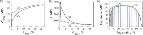
Figure 1(a) shows the monotonic tensile true stress–true strain (σ–) curves in both GS and CG samples. The GS sample shows large tensile ductility comparable to that of CG, but with triple yield strength of CG, which is typical of the excellent combination of strength and ductility in GS metals.[2–8] A transient is visible soon after yielding, characterized by the presence of a short concave segment on the σ– curve.[4] During the transient, the strain hardening rate (Θ) sharply drops at first, which is followed by a rapid up-turn, as shown in Figure 1(b). Figure 1(c) shows the unloading and reloading test hysteresis loops measured at varying tensile strains for both CG and GS samples.

Figure 1. (Colour online) (a) Tensile stress–strain curves in the GS and CG IF steel samples. (b) Strain hardening rate (Θ = dσ/d) vs. strain. (c) The unloading and reloading test hysteresis loops measured at varying tensile strains for both CG and GS samples.

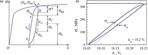
Unloading–reloading was performed at varying tensile strains to investigate the evolution of back stress during tensile test. Figure 2(a) shows schematically the unloading–reloading stress–strain hysteresis loop. As shown, the unloading starts at unloading strains (_u) at point A. The segment AB of the unloading curve is quasi-elastic and caused by stress relaxation [29] or viscous flow of the material.[30,31] The stress drop in this segment is called the thermal component of the flow stress.[24,29] or viscous stress.[30,31] The segment BC is the linear (elastic) part of the unloading stress with an effective unloading Young's modulus of E_u. The point C is called the unloading yielding point, with a stress of σ_u. Similar segments also exist for the reloading curve with EF as the linear (elastic) part of the reloading stress–strain curve with an effective reloading Young's modulus of E_r, which can be assumed equal to E_u because the microstructure is assumed not changed during the unloading–reloading. The point F is called the reloading yielding point, with a stress of σ_r. Figure 2(b) is the measured hysteresis loop from a GS IF steel sample.

Figure 2. (Colour online) (a) The schematic of the unloading–reloading loop for defining the unload yielding σ_u, reload yielding σ_r, back stress σ_b and frictional stress σ_f, effective unloading Young's modulus of E_u, effective reloading Young's modulus of E_r. (b) A measured hysteresis loop from the GS IF steel sample with σ_u and σ_r defined.

From the unloading–reloading hysteresis loop, we can calculate the back stress σ_b, and the frictional stress σ_f. The back stress is always in the opposite direction of the applied stress, while frictional stress is always in the direction that opposes the motion of dislocations. The frictional stress consists of the Peierls stress as well as other stresses that are needed to overcome the dynamic pinning of dislocations such as solute atoms, second phase, forest dislocations, dislocation debris, dislocation jogs, etc.

To derive the equation for calculating the back stress and frictional stress, we first assume that the frictional stress σ_f is a constant during the entire unloading–reloading process. We also assume that the back stress does not change with unloading before the unloading yield point C in Figure 2(a). This assumption is reasonable because the reverse dislocation motion does not start above this point. In other words, GNDs that produce the back stress do not change their density or configuration before the unloading yield, which keeps the back stress approximately constant. This assumption is important and was also adopted by Dickson et al.[29] During the unloading, the back stress is the stress that drives the mobile dislocations to reverse their gliding direction to produce unloading yield. At the unloading yield point C (Figure 2(a)), the applied stress is low enough that the back stress starts to overcome the applied stress and the frictional stress to make dislocations glide backward, that is (1) where σ_u is the unloading yield stress as defined in Figure 2(a).

During the reloading, the applied stress needs to overcome the back stress and the frictional stress to drive the dislocation forward at the reloading yield point F, which can be described as (2) where σ_r is the reloading yield stress as defined in Figure 2(a).

Here again, we assume that the back stress during reloading is the same as the back stress during unloading. This is reasonable because during the unloading–reloading process, dislocation configuration can be considered reversible.[32] Solving Equations (1) and (2) yields (3) and (4)

Equation (3) is similar to an earlier equation proposed for cyclic loading by Cottrell [33] and Kulmann-Wilsdorf and Laird,[32] except they used σ_u0, the initial flow stress at the beginning of the unloading, in place of the σ_r, that is (5) where σ_u0 is the initial unloading stress as defined in Figure 2(a).

We argue that Equation (3) is physically sounder than Equation (5) because we are defining unloading yield and reloading yield using the same criterion, that is, the same deviation of effective Young's modulus as discussed later. It has been recognized that Equation (5) overestimates the back stress, and was later modified by Dickson et al. to include the thermal component of the flow stress:[24,29] (6) where σ* is the thermal component of the flow stress as defined in Figure 2(a),[24,29] which is also called the viscous stress. [31]

Equation (3) is especially suitable for hysteresis loops with positive unloading yield stresses. If the back stress is very small, the unloading yield stress may become negative, in which case σ_u cannot be measured during unloading. However, we expect Equation (3) to be valid if the applied stress is reversed to negative to measure σ_u before the reloading. As discussed later, Equation (3) derived here has an important advantage over previously published Equations (5) and (6): it produces consistent back stress values with much less scatter. In addition, Equations (5) and (6) are physically problematic because they implicitly used different criteria to define the unloading yield and reloading yield, which is physically unjustifiable.

To extract useful data from the unloading–reloading hysteresis loop, one needs to first determine the unloading yield stress σ_u and reloading yield stress σ_r. However, the real hysteresis loop (e.g. Figure 2(b)) is not as well defined as in Figure 2(a), and the practical extraction of the data is not straightforward.[31] The first step is to determine the elastic segments BC as well as its slope (the effective Young's modulus). The unloading yield point C is usually determined by a plastic strain offset in the range of 5 × 10⁻⁶ to 10⁻³, which have been used by different research groups.[24,31,34–37] These offset values are arbitrary and are not well justified. Here we propose to use the deviation of the stress–strain slope from the effective Young's modulus as a physically sound method to determine the yield point. In this study, we choose 5%, 10%, and 15% slope reduction from the effective Young's modulus, E_u. If the strain hardening in the plastically deforming volume is ignored, the slope reduction should be equal to the volume fraction that is plastically deforming. For example, a 10% reduction in E_u means 10% of the sample volume is plastically deforming. We also propose to use E_r = E_u, and the same slope reduction values for determining both the unloading yield point and reloading yield point.

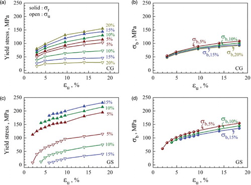
Figure 3 compares the evolution of the unloading yield stress, reloading yield stress, and back stress of the CG and GS IF steel samples with increasing tensile strain at which the unloading was initiated. Several features can be seen from the figure. First, the unloading yield stress is affected more than the reloading yield stress by the slope reduction offset value that is used to determine them (Figure 3(a) and 3(c)). Second, using a larger slope reduction leads to lower unloading yield stress σ_u and higher reloading yield stress σ_r. Part of these variations in σ_u and σ_r caused by the choice of slope reduction cancel each other in Equation (3), which leads to smaller scatter in the calculated back stress using Equation 3 (Figure 3(b) and 3(d)). This is an advantage of Equation (3) for calculating the back stress, as compared with the previously reported Equation (6).[23, 24,29–31] Third, the back stresses in both the CG and GS samples increase with the tensile strain. However, the back stress is higher in the GS sample than in the CG sample. For example, for the 5% slope reduction, the back stress in the GS sample is 10–40% higher than those in the CG sample (the red curves in Figure 3(b) and 3(d)). Fourth, Figure 3(c) and 3(d) shows that if a large slope reduction value is used, the unloading yield stresses for the GS sample at small tensile strains are negative and therefore cannot be measured in the unloading curve. This makes it advantageous to use a smaller slope reduction value in determining the back stress.

Figure 3. (Colour online) Evolution of (a) unloading yield stress σ_u and reloading yield stress σ_r and (b) back stress with increasing unloading strain _u for CG IF steel, and the evolution of (c) unloading/reloading yield stresses and (d) back stress with increasing _u for GS IF steel. σ_b,5% represents the back stress calculated using 5% slope reduction from the effective Young's modulus.

For valid and easy comparison, we propose that the slope reduction value for calculating the back stress is marked in the symbol. For example, σ_b,5% represents back stress calculated using 5% slope reduction from the effective Young's modulus, as shown in Figure 3(b) and 3(d). Of course, there exist uncertainties in defining E_u, E_r, and the corresponding slope reductions due to the difficulties for determining the linear parts of both unloading and reloading curves; however, the consequences of these uncertainties appear to be small due to the method we used.

As shown in Figure 4(a), the frictional stress σ_f calculated using Equation (4) is very scattered. A larger slope reduction value leads to significantly higher σ_f. For example, for the CG sample, the σ_f calculated using 20% slope reduction is many times larger than those calculated using the 5% slope reduction. This is because Equation (4) adds the absolute values of σ_u and σ_r variations together instead of making them cancel each other as in Equation (3). Therefore, the frictional stress σ_f calculated using Equation (4) is not quantitatively dependable. Nevertheless, Figure 4(a) consistently shows that for any slope reduction value, the calculated frictional stress is higher in the GS sample than in the CG sample. This is due to the higher dislocation density in the GS sample than in the CG sample.[3,4]

Figure 4. (Colour online) The frictional stress σ_f vs. tensile strain _true for the GS and CG IF steel samples calculated according to Equation (4). (b) The distinct back stress hardening in GS IF steel. denotes the back stress hardening rate calculated using 5% slope reduction from the effective Young's modulus.

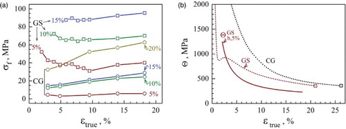
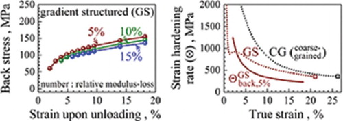
Figure 4(b) shows that the GS sample has much higher back stress strain-hardening than the CG sample due to the heterogeneous microstructure, especially in the transient range that correlates to Θ up-turn. This indicates that the back stress strain-hardening has significant contribution to the observed Θ up-turn. The rapid back stress increase right after the yielding of the GS sample is also obvious in Figure 3(d). The observed Θ up-turn has been attributed to fast dislocation accumulation due to the back stress strain-hardening after the initial exhaustion of mobile dislocations.[4] The high back stress associated with the observed Θ up-turn observed here suggests that a large quantity of GNDs is accumulated at this stage. Since the GNDs are associated with the strain gradient in the sample, this observation also suggests that there was a quick increase in the strain gradient at the beginning of the plastic deformation of the GS IF steel. This is understandable because this is at the deformation stage in which the NS surface layers just started to become unstable and the lateral (perpendicular to the tensile direction) stresses start to reverse their directions.[3,4] Specifically, the surface NS layers transit from compressive lateral stress to tensile laterals stress, while the central larger grained layer transits in an opposite way. Such a transition is expected to increase the strain gradient.

In summary, it is found that the GS IF steel developed strong back stress strengthening and back stress strain-hardening during tensile testing, which arise from the plastic incompatibilities due to its microstructural heterogeneity. The high back stress near the beginning of the plastic deformation of the GS IF steel samples should have contributed to the observed synergetic strengthening,[3] while the high back stress hardening should have contributed to the observed high ductility.[4] The equation derived and the procedure proposed in this work for calculating the back stress from the unloading–reloading hysteresis loop produces more consistent back stress value than what is previously reported.

Acknowledgements

This work was supported by the National Natural Science Foundation of China under Grant numbers (11572328, 11072243, 11222224, 11472286, and 51471039); and 973 Projects under Grant numbers (2012CB932203, 2012CB937500, and 6138504). Y.T.Z. is funded by the US Army Research Office (W911 NF-12–1–0009), the US National Science Foundation (DMT-1104667), and by the Jiangsu Key Laboratory of Advanced Micro&Nano Materials and Technology, Nanjing Univ of Sci and Technol.

Disclosure statement

No potential conflict of interest was reported by authors.

References

- Lu K. Making strong nanomaterials ductile with gradients. Science. 2014;345(6203):1455–1456. doi: 10.1126/science.1255940
- Fang TH, Li WL, Tao NR, Lu K. Revealing extraordinary intrinsic tensile plasticity in gradient nano-grained copper. Science. 2011;331(6024):1587–1590. doi: 10.1126/science.1200177
- Wu XL, JIang P, Chen L, et al. Synergetic strengthening by gradient structure. Mater Res Lett. 2014;2(4):185–191. doi: 10.1080/21663831.2014.935821
- Wu XL, Jiang P, Chen L, Yuan FP, Zhu YT. Extraordinary strain hardening by gradient structure. Proc Natl Acad Sci USA. 2014;111(20):7197–7201. doi: 10.1073/pnas.1324069111
- Jerusalem A, Dickson W, Perez-Martin MJ, Dao M, Lu J, Galvez F, Grain size gradient length scale in ballistic properties optimization of functionally graded nanocrystalline steel plates. Scr Mater. 2013;69(11):773–776. doi: 10.1016/j.scriptamat.2013.08.025
- Wang HT, Tao NR, Lu K. Architectured surface layer with a gradient nanotwinned structure in a Fe-Mn austenitic steel. Scr Mater. 2013;68(1):22–27. doi: 10.1016/j.scriptamat.2012.05.041
- Kou HN, Lu J, Li Y. High-strength and high-ductility nanostructured and amorphous metallic materials. Adv Mater. 2014;26(31):5518–5524. doi: 10.1002/adma.201401595
- Wei YJ, Li YQ, Zhu LC, et al. Evading the strength-ductility trade-off dilemma in steel through gradient hierarchical nanotwins. Nat Comm. 2014;5: Article no. 3580.
- Ma XL, Huang CX, Xu WZ, Zhou H, Wu XL, Zhu YT. Strain hardening and ductility in a coarse-grain/nanostructure laminate material. Scr Mater. 2015;103:57–60. doi: 10.1016/j.scriptamat.2015.03.006
- Fang TH, Tao NR, Lu K. Tension-induced softening and hardening in gradient nanograined surface layer in copper. Scr Mater. 2014;77:17–20. doi: 10.1016/j.scriptamat.2014.01.006
- Weertman JR. Retaining the nano in nanocrystalline alloys. Science. 2012;337(6097):921–922. doi: 10.1126/science.1226724
- Chookajorn T, Murdoch HA, Schuh CA. Design of stable nanocrystalline alloys. Science. 2012;337(6097):951–954. doi: 10.1126/science.1224737
- Zhang K, Weertman JR, Eastman JA. Rapid stress-driven grain coarsening in nanocrystalline Cu at ambient and cryogenic temperatures. Appl Phys Lett. 2005;87(6): Article no. 061921. doi: 10.1063/1.2008377
- Zhang K, Weertman JR, Eastman JA. The influence of time, temperature, and grain size on indentation creep in high-purity nanocrystalline and ultrafine grain copper. Appl Phys Lett. 2004;85:5197–5199. doi: 10.1063/1.1828213
- Legros M, Gianola DS, Hemker KJ. In situ TEM observations of fast grain-boundary motion in stressed nanocrystalline aluminum films. Acta Mater. 2008;56(14):3380–3393. doi: 10.1016/j.actamat.2008.03.032
- Liao XZ, Kilmametov AR, Valiev RZ, Gao HS, Li XD, Mukherjee AK, Bingert JF, Zhu YT. High-pressure torsion-induced grain growth in electrodeposited nanocrystalline Ni. Appl Phys Lett. 2006;88: Article no. 021909. doi: 10.1063/1.2159088
- Li WB, Yuan FP, Wu XL. Atomistic tensile deformation mechanisms of Fe with gradient nano-grained structure. AIP Advances. 2015;5(8): Article no. 087120. doi: 10.1063/1.4928448
- Li JJ, Chen SH, Wu XL, Soh AK. A physical model revealing strong strain hardening in nano-grained metals induced by grain size gradient structure. Mater Sci Eng A. 2015;620:16–21. doi: 10.1016/j.msea.2014.09.117
- Llorca J, Needleman A, Suresh S. The Bauschinger effect in whisker-reinforced metal-matrix composites. Scr Metall Mater. 1990;24(7):1203–1208. doi: 10.1016/0956-716X(90)90328-E
- Sinclair CW, Saada G, Embury JD. Role of internal stresses in co-deformed two-phase materials. Philos Mag. 2006;86(25–26):4081–4098. doi: 10.1080/14786430600654438
- Thilly L, Van Petegem S, Renault PO, Lecouturier F, Vidal V, Schmitt B, Van Swygenhoven H. A new criterion for elasto-plastic transition in nanomaterials: application to size and composite effects on Cu-Nb nanocomposite wires. Acta Mater. 2009;57(11):3157–3169. doi: 10.1016/j.actamat.2009.03.021
- Calcagnotto M, Adachi Y, Ponge D, Raabe D. Deformation and fracture mechanisms in fine- and ultrafine-grained ferrite/martensite dual-phase steels and the effect of aging. Acta Mater. 2011;59:658–670. doi: 10.1016/j.actamat.2010.10.002
- Wu XL, Yang MX, Yuan FP, Wu GL, Wei YJ, Huang XX, Zhu YT. Heterogeneous lamella structure unites ultrafine-grain strength with coarse-grain ductility. Proc Natl Acad Sci USA. 2015;112(47):14501–14505. doi: 10.1073/pnas.1517193112
- Feaugas X. On the origin of the tensile flow stress in the stainless steel AISI 316L at 300 K: back stress and effective stress. Acta Mater. 1999;47(13):3617–3632. doi: 10.1016/S1359-6454(99)00222-0
- Ashby MF. The deformation of plastically non-homogeneous materials. Philos Mag. 1970;21(170):399–424. doi: 10.1080/14786437008238426
- Gao H, Huang Y, Nix WD, Hutchinson JW. Mechanism-based strain gradient plasticity - I Theory. J Mech Phys Solids. 1999;47(6):1239–1263. doi: 10.1016/S0022-5096(98)00103-3
- Gao HJ, Huang YG. Geometrically necessary dislocation and size-dependent plasticity. Scr Mater. 2003;48(2):113–118. doi: 10.1016/S1359-6462(02)00329-9
- Lu K, Lu J. Nanostructured surface layer on metallic materials induced by surface mechanical attrition treatment. Mater Sci Eng A. 2004;375–377:38–45. doi: 10.1016/j.msea.2003.10.261
- Dickson JI, Boutin J, Handfield L. A comparison of two simple methods for measuring cyclical internal and effective stresses. Mater Sci Eng. 1984;64(1):L7–L11. doi: 10.1016/0025-5416(84)90083-1
- Fournier B, Sauzay M, Caes C, Mottot M, Noblecourt A, Pineau A. Analysis of the hysteresis loops of a martensitic steel - Part II: study of the influence of creep and stress relaxation holding times on cyclic behaviour. Mater Sci Eng A. 2006;437:197–211. doi: 10.1016/j.msea.2006.08.087
- Fournier B, Sauzay M, Caes C, Noblecourt M, Mottot M. Analysis of the hysteresis loops of a martensitic steel - Part I: study of the influence of strain amplitude and temperature under pure fatigue loadings using an enhanced stress partitioning method. Mater Sci Eng A. 2006;437:183–196. doi: 10.1016/j.msea.2006.08.086
- Kuhlmann-Wilsdorf D, Laird C. Dislocation behavior in fatigue II. Friction stress and back stress as inferred from an analysis of hysteresis loops. Mater Sci Eng. 1979;37(2):111–120. doi: 10.1016/0025-5416(79)90074-0
- Cottrell AH. Dislocations and plastic flow in crystals. Oxford: Clarendon Press; 1953.
- Delobelle P, Oytana C. The study of the laws of behavior at high-temperature, in plasticity-flow, of an austenitic stainless-steel (17–12-Sph). J Nucl Mater. 1986;139(3):204–227. doi: 10.1016/0022-3115(86)90174-1
- Risbet M, Feaugas X, Clavel M. Study of the cyclic softening of an under-aged gamma'-precipitated nickel-base superalloy (Waspaloy). Journal De Physique IV. 2001;11(PR4):293–301. doi: 10.1051/jp4:2001436
- Guillemer-Neel C, Feaugas X, Clavel M. Mechanical behavior and damage kinetics in nodular cast iron: part II. Hardening and damage. Metall Mater Trans A. 2000;31(12):3075–3085. doi: 10.1007/s11661-000-0086-2
- Morrison DJ, Jia Y, Moosbrugger JC. Cyclic plasticity of nickel at low plastic strain amplitude: hysteresis loop shape analysis. Mater Sci Eng A. 2001;314(1):24–30. doi: 10.1016/S0921-5093(00)01914-6