Observation of dynamical transformation plasticity in metallic nanocomposites through a precompiled machine-learning algorithm

Abstract

Machine learning capabilities combined with in-situ TEM measurements on aluminum-carbon nanotube composites reveal a new deformation sequence of dislocation gliding and pinning, a quiescent period, and finally a sudden release of localized strain. We propose a plastic deformation mechanism operating with three essential distinguishing characteristics: correlation of spatially localized microstrustural defects on the scale of nanometers, barrier-activation process of shear stress loading giving rise to strain response, and transient response on the time scale of seconds. Implications regarding plasticity carriers known to operate in crystalline media and in amorphous solids such as metallic glasses are discussed.

GRAPHICAL ABSTRACT

IMPACT STATEMENT

A machine learning augmented investigation reveals the presence of cut-resistant nanotubes tilts the energy balance from crystal plasticity to more amorphous-like deformation mechanisms, particularly localized, transient strain observed in aluminum.

KEYWORDS:

• Transformation plasticity
• Heterogeneous materials
• Nanocomposite
• Shear transformation
• Carbon nanotubes (CNTs)

Introduction

We report here a high-resolution, in situ TEM study of mechanically loaded aluminum carbon nanotube (CNT) composites. The work is a follow up on our prevous finding of strength increasing with nanotube concentration, while ductility was minimally affected [1]. This behavior was rationalized by considering dislocation effects in a crystalline material. In contrast, present work is motivated by obtaining a mechanistic explanation of the apparent high ductility without assuming the deforming microstructure to be fully crystalline. To achieve this goal we rely on improving image refinement and analysis techniques through a machine-learning approach. As we show below, one is now able to directly visualize the spatio-temporal evolution of a 3D reconstructed strain map on the scale of nanometer-seconds in sufficient detail to suggest the operation of a new type of plastic deformation process. Interpretation of this mechanism shows that it should not be associated with a single defect, such as a dislocation. Rather, the process appears to be a sequence of microstructural reponses with characteristic spatial and temporal extents on the orders of nanometers and seconds. Relative to existing plastic deformation mechanisms, the most relevant ones are those introduced for amorphous solids, based on free-volume diffusion [2], shear transformation deformation [3], and a hybrid of these two [4].

To take advantage of recent improvements made in computer vision [5,6], our programming language of choice is Julia, an open-source, dynamic language that is exceptionally fast and compatible with other languages such as Python, Matlab, and C++ [7]. It is user-friendly, self-optimizing, and well-suited for scientific machine learning applications [8,9]. In this work, we utilize Julia to capture the dynamic details of deformation plasticity in nanocomposites synthesized at a non-equilibrium state by analyzing in situ TEM videos and images of the composite during deformation.

The first challenge was to identify and quantify the features in the video data of limited resolution. We implemented an image filter based on compressed sensing algorithms in Julia, not only for noise reduction but also to construct a 3D nanostructure surface to visualize the spatio-temporal development of a strain-response map of the specimen. We characterize defect dynamics initiated on a surface notch under stress in the vicinity of CNT. Localized strains can be resolved at the <50 nm length scale and followed for time periods of 40 s. Our findings have implications regarding the nature of deformation mechanisms associated with yielding in complex, heterogeneous nanostructures. Such a deformation mechanism at the nanoscale pertains to current concepts of dynamical heterogeneities discussed in condensed matter physics and soft-matter rheology communities [10]. We discuss how to characterize such transient and highly localized nanoscale events and consider their possible connections to existing perspectives and models, such as the weakening mechanism of transformation plasticity according to Poirier [11], the shear transformation model proposed by Argon [3], and shear transformation zones (STZ) introduced by Falk and Langer [4].

Methods

The data we analyze in this study are in situ TEM video images reported in a previous publication [1], available in the data repository for this manuscript [12]. The low-resolution video was separated into individual frames in order to extract information from its constituent, noisy images. We constructed a data processing pipeline to enhance the signals through custom-built algorithms assembled from open-source code written in Julia, consisting of the Michigan image reconstruction toolbox (MIRT) [13] and Makie [14]. Noise filtering and defect features were identified from k-space image reconstruction using the MIRT algorithm [5]. A conjugate gradient (CG) minimizer was used to smooth images. Since a quadratic regularizer,$\beta \frac{1}{2}||Tx|{|}_2^2$, blurred the edges when using a finite difference K×N matrix transformation (T), we used the non-quadratic regularizer to reduce blur and clarify features. The cost function we adopted is: (1) $\hat{x}=argmin\mathrm{\Psi }(x)\stackrel{\Delta }{=}\frac{1}{2}{A}_x-y_2^2+\beta \mathrm{\Psi }(Tx)$(1) To define the proper regularization and potential function to visualize features before processing the video, we used Julia's built-in interactive slider bar. We further reconstructed 3D color-coded surfaces to identify and label features in the TEM video.

We contrast the present method with neural network-based super-resolution methods [15,16] for a direct comparison to relevant, state of the art image analysis tools. An upscaled image is created from our low-resolution TEM image using a convolutional neural network (CNN) through very deep learning super-resolution (VDSR) [17], enhanced deep learning super-resolution (EDSR) [18], and a fast super-resolution convolutional neural network (FSRCNN) [17]. In addition, we ran a sparse and low-ranking tensor (SALT)-based temporal denoising algorithm, which utilized feature-tracking k-nearest neighbors (KNN) machine learning [19]. Pretraining was performed with data in the ImageNet repository or measured TEM data.

Results

Data processing pipeline

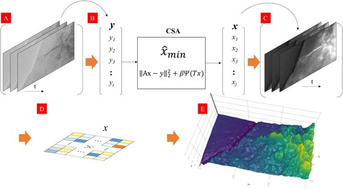
Our goal of analyzing and segmenting raw experimental data is to characterize the mechanisms governing defect evolution in our system. These observations can be used to validate current understanding of the governing mechanisms, or to identify new mechanisms previously not considered. In either case, the objective is to arrive at interpretations of mechanistic behavior useful for materials discovery, design, and testing. Figure 1 shows a schematic of the image processing pipeline, in which in situ TEM video is treated by a compressed sensing algorithm (CSA) [20,21] to enhance limited signal information through k-space reconstruction with the non-quadratic edge-preserving regularizer mentioned above,$\beta \mathrm{\Psi }(Tx)$, where y is the k-space noise vector obtained from image frames in Figure 1A. The y-vector acts as input data to create the new data set, x, through the CSA (Figure 1B). The cost function ${\hat{x}}_{min}$ generates the output image vector, x, through multiple iterations. The cost function minimization process reduces noise in the data; thus, the x-vector contains processed image data with clean and enhanced signals (Figure 1C). CSA is particularly useful for reconstructing data from a limited set of measurements, especially when high-resolution reference data are not available, such as those collected in this study. The vector array, x, is further pixelated into 2D maps where color blocks indicate individual pixels in the image (Figure 1D) to plot the surface to better visualize features. Finally, a 3D surface reconstruction with a color-coded topology proportional to pixel intensity is obtained to enable the direct physical interpretation of dynamical processes in our nanocomposite system (Figure 1E).

Figure 1. Schematic of the data processing pipeline for image frames from in situ TEM videos. This platform facilitates information extraction from low-quality images through sparse and compressed sensing algorithms and 3D visualization. (A) image frames in the video, (B) sparse and compressed sensing k-space reconstruction with an edge-preserving regularizer, (C) 2D image reconstruction, and (D) 2D vector map for 3D reconstruction. (E) a color-coded 3D surface plot to visualize the four stages of microstructure evolution in nanocomposites.

Defect-feature identification using the compressed sensing algorithm

Resolution enhancement is an ever-present challenge in defect-feature identification. We have used a pretrained super-resolution (SR) package [15], based on a generative adversarial network (GAN) algorithm [22]. In so doing we have made comparisons with other data processing pipelines with advanced SR, conventional CNN, and KNN-based denoising algorithms. The original frame (Figure 2A) in the video was treated as input in the comparison.

Figure 2. Defect feature identification through Julia-compressed sensing and state-of-art super-resolution (SR) computer vision algorithms. (A) Raw TEM images show a faint, darker circle feature in the white box. (B) Denoising with CSA using line-search optimized gradient 2D reconstructions and edge-preserving regularization (see Figure 1). The feature in the white box shows noticeable enhancement with a clear boundary after CSA in Julia. However, SR with convolutional neural networks in (C) VSDR, (D) FSRCNN, and (E) EDSR show no significant enhancement. Furthermore, the k-nearest neighbors video denoising algorithm (F) temporal SALT shows limited enhancement. After the CSA process of 2D reconstruction in (B), the 3D surface was color coded to identify and label the features. Based on physical attributes such as size and shape, we interpret the identified features to be Notch, Dislocation, CNT, delocalized strain, and Cut. All scale bars are 10 nm.

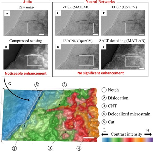
We further quantified the efficacy of our image processing algorithm via three methods: (1) Contrast ratio between features and background, (2) Signal-to-noise ratio (SNR), and (3) Feature sharpness. The CSA enhances the signal within relevant features by ∼50%, especially for the shear transformation region, enabling easier machine-vision identification of these regions. In addition, the CSA both reduces the noise and enhances the signal. For example, the standard deviation in the base area is ten times larger in before and after CSA processing. Thus, CSA significantly increases the SNR. The feature sharpness is about 2.5 times higher after the CSA process, indicating that it effectively identifies hidden features in noisy, low-resolution images. The supplementary information for this manuscript contains more details about this comparison.

Stages of dynamical defect evolution

The original frame shows only limited details of the movements of the individual defect features we would like to decipher. As data are processed along the pipeline (Figure 1), further defect features become more noticeable, see for example, the region highlighted within the white box in Figure 2B. In contrast to CSA processing in Julia, denoising/upscaling using SR with CNN-VSDR (Figure 2C), FSRCNN (Figure 2D), and EDSR (Figure 2E) show no significant improvements. Moreover, the KNN video denoising algorithm using temporal SALT (Figure 2F) also shows only limited enhancement. We have found that at the nanometer scale, it is much more difficult to pre-train images compared to the meter scale as a result of greater feature complexity, more limited complementary information, and larger variance of images in the TEM and SEM training datasets as compared to meter-scale photo training datasets (e.g. obtained from Google). Defect-feature identification at the nanoscale therefore requires greater differentiation between microstructural features and various defect interactions, many of which could lead to mapping to the same observed features if distinguishing information is insufficient.

The data processing pipeline enabled several features to be deciphered and tracked over time in what still remain as low-resolution images. Temporal tracking of the evolution of features is vital in resolving dynamical processes at the nanoscale. After measuring properties such as yield strength at various times, the correlation between time-dependent structures and corresponding material property changes leads to a dynamic structure–property relationship which then allows us to gain a deeper understanding of the underlying deformation mechanisms that can operate in metallic nanocomposites.

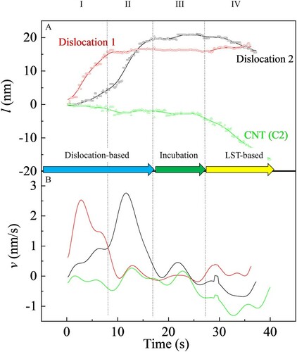
In the specific case of deforming CNT nanocomposites, their structural evolution separates naturally into four stages of nanostructure time evolution, as suggested by the reconstructed 2D/3D video frames and processed data in Figure 3 . By following the variation in length and speed of two discernible dislocations and the lower CNT from Figure 2, we see the deformation sequence is composed of stages: (I) gliding of dislocation , (II) gliding of dislocation , (III) incubation period of little activity at the nanostructure level, and (IV) a plastic deformation process of sudden strain release in a localized region. For stage IV, we suggest calling the process localized shear transient (LST). Besides Figure 3, our characterization is critically facilitated by a 40-second video (see https://youtu.be/64jmLfbB5lQ), which is a key result of the image processing improvement undertaken in this work.

Figure 3. Comprehensive time evolution data for dislocations and lower CNT movement in an aluminum CNT composite. (A) Displacement of the dislocations and lower CNT as a function of time. (B) The velocity of features indicates correlation between velocity changes, implying that the features are coupled with each other. The red line indicates dislocation 1 gliding, while the black line indicates dislocation 2 gliding. Dislocation 1 is the active strain carrier in stage I, whereas dislocation 2 is the active strain carrier in stage II. Stage III shows an incubation time of about 10 s before the localized shear transient (LST). At stage IV, the lower CNT is moving; which indicates further deformation (Figure 4 & video 2).

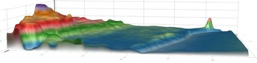
We continue by examining evolution of our 3D reconstructed strain map surface duing stage IV deformation (see https://youtu.be/geNUsbkjbgM). Figure 4 follows the nanostructure changes at four instants in time. At 29.5 sec (Figure 4A), the surface topology suggests a spatial demarcation has already taken place in that there exists a region of high contrast intensity (orange-red) on the right side of the figure, adjacent to a region of similar extent but having low intensity (green–blue) on the left side. We give below an interpretation of what we believe is the onset of a LST deformation. At 33.5 sec (Figure 4B), the topology has apparently ‘ripened’ with the nanostructure becoming somewhat cleaner as in recovery after a sudden change. Relative to Figure 4A one can detect a shift (shear or rotation) of the landscape as indicated by the dashed line and the arrows. At 36 sec, the relaxation of surface features (undulations) continues with the separation between high/low contrast regions becoming even more prominent. If one applies an analogy of a volcanic eruption to Figure 4A, then Figures 4B and C may be regarded as the ‘aftershocks’ of a sudden blowout or seismic event. Finally, at 41 sec (Figure 4D), one sees the termination or pause of the nanostructure change initialized at 29.5 sec. Comparing Figure 4D with Figure 4A, one can appreciate how the ridge of high strain (purple-topped orange region) is formed over a relaxation duration of 10.5 s.

Figure 4. Visualization of evolution of reconstructed surface during stage IV of aluminum-CNT composite deformation. Panel (A) shows the surface topology in strain contrast mapping at 29.5 s. The color indicates contrast intensity, according to the legend bar at lower-left. Four characteristic, topological features may be identified: a plateau area of high strain (yellow-red), a shear line (green), base area of low strain (blue), and a CNT (green surrounded by red, see also panel (D)). Panel (B) shows how the topology on the plateau evolves over 4 s from its early-stage appearance. Note the line of shear (dashed line) and strain redistribution (arrows). At 36 s, panel (C) indicates strain redistribution (self-organization) continuing with significant changes in both the plateau boundary and intensity distribution. After another 5 s, panel (D) shows the plateau topology seems to have converged, as is the case for the surrounding areas of lower strain. Other nearby defect features we have previously noted (recall Figure 2) are indicated.

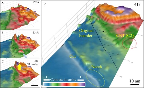
The experimental results presented in Figures 2–4 and the two videos collectively suggest an interpretation of a plastic deformation process pertaining to the spatial and temporal behavior of the deformation response identified during stage IV. As can be seen in Figure 4, there are three distinguishing features which together characterize a new type of plastic deformation mechanism, which we have denoted as LST. First is a spatial localization on the scale of ∼10 nm. By this we mean an assembly of defects on the nanoscale such as a carbon nanotube (C1) which could play the role of an obstacle to dislocation motion, or another carbon nanotube (C2) which could trigger sudden strain production (see Figure 4A). Second, the dominant deformation involved is a shear process such as the shift manifested in Figure 4B (dashed line and arrows). Last, the mechanism is time-dependent as well as of finite duration, and is therefore a transient process in local barrier activation and relaxation (Figure. 4C and D). These three characteristics lead us to interpret the behavior observed during stage IV as the onset of a LST event and its subsequent evolution.

Associated with the interpretation of LSTs is the question of how does it differ from other plastic deformation processes. Relative to the concept of ‘transformation plasticity' [11,23], we note that an LST does not require crystallinity. It can take place in local regions of disorder or free volume where jamming or sudden release (activation) of stress or strain can occur. There are similarities between LSTs and the defect STZ widely invoked in describing deformation and transport in amorphous solids [4,24]. One can also consider similarities between LSTs and two early models of plastic deformation in metallic glasses, one based on the concept of free-volume diffusion [2] and another on shear transformation [3,25]. These connections are worthy to be explored further in the context of rheological phenomena such as creep, discontinuous shear thickening, and the flow of dense suspensions, as LSTs may be active in viscous liquids and amorphous solids.

Conclusions

We have presented experimental findings that point to a new type of mechanism of plasticity via localized strain production, which we denote as a localized shear transient (LST). Our experimental data explicitly show a sequence of microstructural evolution on the nanometer scale over a duration of 40 s. Of particular significance are the details of surface relaxation behavior seen in Figure 4. In the form of 3D surface reconstruction with color coding, we have observed a sudden strain relaxation (barrier activation) event over a local region, and its subsequent effects on the reconstructed surface.

Overall the essential features of an LST consist of (1) correlation of local defects on the nanometer scale, (2) plasticity response triggered by shear activation, and (3) a transient barrier-activation process on the time scale of seconds. It should also be noted that the LST is not a standalone, stationary ‘unit process,’ rather it is a dynamical response with a ‘precursor memory’ and consequential evolution.

Acknowledgment

We acknowledge Ju Li for supporting this work, Alan Edelman for introducing us to Julia, Virginia Spanoudaki for sharing with us her expertise in data analysis through computer vision, Valentin Churavy for helping us to build the data analysis algorithm used in this work, Chris Rackauckas for guidance pertaining to scientific machine learning, and Viral Shah for sustained guidance to the Julia group at MIT. While the interpretations and discussions are our own, we have benefitted from conversations with Ting Zhu, Wei Cai, and Ken Kamrin. K.P. So was supported by the US DOE Office of Nuclear Energy's NEUP Program under Grant No. DE-NE0008827 and NSUF for facility access via RPA-18-14783. M.L. was partially supported by U.S. Department of Energy (DOE) Award No. DE-SC002194, National Science Foundation (NSF) DMR-2118448, and Norman C. Rasmussen Career Development Chair. 

Disclosure statement

No potential conflict of interest was reported by the author(s).

References

- So KP, Liu X, Mori H, et al. Ton-scale metal–carbon nanotube composite: The mechanism of strengthening while retaining tensile ductility. Extreme Mech Lett. 2016;8:245–250.
- Spaepen, F. A microscopic mechanism for steady state inhomogeneous flow in metallic glasses. Acta Metall. 1977;25(4):407–415.
- Argon A. Plastic deformation in metallic glasses. Acta Metall. 1979;27(1):47–58.
- Falk ML, Langer JS. Dynamics of viscoplastic deformation in amorphous solids. Phys Rev E. 1998;57(6):7192.
- Fessler JA. Optimization methods for magnetic resonance image reconstruction: Key models and optimization algorithms. IEEE Signal Process Mag. 2020;37(1):33–40.
- Ravishankar S, Ye JC, Fessler JA. Image reconstruction: from sparsity to data-adaptive methods and machine learning. Proc IEEE. 2019;108(1):86–109.
- Bezanson J, Karpinski S, Shah VB, et al. Julia: A fast dynamic language for technical computing. arXiv. 2012: 1209.5145.
- Perkel JM. Julia: come for the syntax, stay for the speed. Nature. 2019;572(7768):141–143.
- Bezanson J, Edelman A, Karpinski S, et al. Julia: A fresh approach to numerical computing. SIAM Rev. 2017;59(1):65–98.
- Cao P, Short MP, Yip S. Potential energy landscape activations governing plastic flows in glass rheology. Proc Natl Acad Sci USA. 2019;116(38):18790–18797.
- Poirier J. On transformation plasticity. J Geophys Res: Solid Earth. 1982;87(B8):6791–6797.
- Julia code and TEM data repository. (2021). https://www.dropbox.com/sh/6q0j45dw8abjyee/AACS0QkWcOrLWABCoYEFpAQwa?dl=0.
- Fessler JA. Michigan image reconstruction toolbox. Ann Arbor (MI): Jeffrey Fessler; 2018. https://web.eecs.umich.edu/∼fessler/code.
- Danisch S, Krumbiegel J. Makie. jl: flexible high-performance data visualization for julia. J Open Source Softw. 2021;6(65):3349.
- Ledig C, Theis L, Huszár F, et al., editors. Photo-realistic single image super-resolution using a generative adversarial network. Proceedings of the IEEE conference on computer vision and pattern recognition; 2017.
- Dong C, Loy CC, Tang X. Accelerating the super-resolution convolutional neural network. In: European conference on computer vision. Cham: Springer; 2016, October. pp. 391–407.
- Kim J, Lee JK, Lee KM. editors. Accurate image super-resolution using very deep convolutional networks. Proceedings of the IEEE conference on computer vision and pattern recognition; 2016.
- Lim B, Son S, Kim H, et al. editors. Enhanced deep residual networks for single image super-resolution. Proceedings of the IEEE conference on computer vision and pattern recognition workshops; 2017.
- Wen B, Li Y, Pfister L, et al. editors. Joint adaptive sparsity and low-rankness on the fly: an online tensor reconstruction scheme for video denoising. Proceedings of the IEEE international conference on computer vision; 2017.
- Donoho DL. Compressed sensing. IEEE Trans Inf Theory. 2006;52(4):1289–1306.
- Eldar YC, Kutyniok G. Compressed sensing: theory and applications. Cambridge university press; 2012.
- Goodfellow IJ, Pouget-Abadie J, Mirza M, et al. Generative adversarial nets. Adv Neural Inf Process Syst. 2014;27:2672.
- Poirier J. Creep of crystals. X: Cambridge University Press; Ch. 8; 2009.
- Schuh CA, Hufnagel TC, Ramamurty U. Mechanical behavior of amorphous alloys. Acta Mater. 2007;55(12):4067–4109.
- Demkowicz MJ, Argon AS. High-density liquid-like component facilitates plastic flow in a model amorphous silicon system. MRS Online Proceedings Library (OPL). 2003: 806.