Multiscale coupled three-dimensional model analysis of the tsunami flow characteristics around the Kamaishi Bay offshore breakwater and comparisons to a shallow water model

ABSTRACT

A two-way coupled two-dimensional (2DH) shallow water to three-dimensional (3D) Navier–Stokes equation model, named 2-way Coupled Long Wave to Navier–Stokes 3D (2CLOWNS-3D), is applied to the 2011 Tohoku-oki Earthquake Tsunami in Kamaishi Bay, Japan. 2CLOWNS-3D simulates the entire evolution of the tsunami from its source to inundation at the coast, in which the 3D model component is used to model the flow through the submerged opening of a large-scale offshore tsunami breakwater. 2CLOWNS-3D is compared with a 2DH model simulation in order to identify where it becomes beneficial. It is found that flow rates through the submerged breakwater opening, and thus the resulting inundation heights, are similar between 2DH and 2CLOWNS-3D model simulations when an appropriate momentum dispersion coefficient is applied to the former. However, significant differences between the model simulations are identified in relation to; hydrodynamic forces acting on the submerged caissons, velocities in the large-scale jet structure emanating from the breakwater, and bed shear stresses in the vicinity of the breakwater. Furthermore, the characteristics of the large-scale jet structure simulated by the 3D model are reasonable when employing the realizable k-ε turbulence closure. Our results demonstrate the practical merit of 2CLOWNS-3D for simulating complex geophysical scale flows.

KEYWORDS:

• Two-way coupling
• shallow water equations
• Navier–Stokes equations
• offshore breakwater
• 2011 Tohoku-oki Earthquake Tsunami

1. Introduction

The March 2011 Tohoku-oki Earthquake Tsunami event in northeastern Japan caused catastrophic widespread damage resulting in 15,895 fatalities with an additional 2539 missing (National Police Agency of Japan, 2018). In total, 121,776 buildings fully collapsed, 280,923 buildings partially collapsed, and 116 bridges were damaged as of March 9, 2018 (National Police Agency of Japan, 2018). The direct economic damage in just the first year after the accident has been estimated at US$221 billion (Kajitani, Chang, and Tatano, 2013).

Due to its long history of tsunami disasters, Japan may have been one of the most prepared nations with regard to its construction of coastal protection structures, e.g. seawalls, gates, offshore tsunami breakwaters, and planted trees to act as natural tsunami barriers. Suppasri et al. (2013) highlight examples where significant damage occurred during the 2011 tsunami event for each such coastal protection structure. For example, the large-scale offshore tsunami breakwater in Kamaishi Bay, located on the Sanriku ria coast in Iwate Prefecture, was constructed in a water depth of 63 m, making it the deepest caisson breakwater in the world (Tanimoto and Takahashi, 1994). It consisted of a pair of offshore tsunami breakwaters with lengths of 990 and 670 m connected by a 300-m long fully submerged opening, and it was expected to provide full protection to the Kamaishi district. Nevertheless, even this breakwater succumbed to the force of the tsunami where many caissons either completely slid out or leaned out of position (Arikawa et al., 2012; Arikawa and Oie, 2015). Thus, it is important in the consideration of future events to analyze the effects of coastal protection structures on the hydrodynamic aspects of tsunamis in greater detail. This will allow us to more effectively design resilient structures capable of withstanding various degrees of tsunami strengths that can mitigate the energy of tsunamis to its maximum potential.

Previous studies have investigated the influence of the Kamaishi Bay offshore tsunami breakwater on tsunami heights, inundation depths and current velocities along the Kamaishi Bay coast (Arikawa and Oie, 2015; Mori, Yoneyama, and Pringle, 2015; Ozer Sozdinler et al., 2015; Pringle and Yoneyama, 2013; Takahashi et al., 2011) predominantly using horizontal two-dimensional (2DH) nonlinear shallow water equation (NSWE) models. A two-way coupled 2DH NSWE to three-dimensional (3D) Navier–Stokes model has also been employed (Mori, Yoneyama, and Pringle, 2015; Pringle and Yoneyama, 2013). The breakwater has been shown to result in an approximately 25–40% reduction to the tsunami heights between elevations offshore of the breakwater and onshore in the bay (Mori, Yoneyama, and Pringle, 2015). Moreover, according to Arikawa and Oie (2015), the breakwater resulted in a 55% reduction to the mean maximum inundation depths in Kamaishi Bay versus the case without a breakwater. However, this reduction rate is less than the possible 70% reduction to inundation depths if the breakwater was not partially damaged (Arikawa and Oie, 2015). Although in most locations the current speeds were decreased, simulations suggest that the breakwater increased current speeds in some residential areas due to the funneling of the wave through the submerged breakwater opening (Ozer Sozdinler et al., 2015).

In addition to the large-scale impacts of coastal structures on inundation heights and current speeds overland, it is also increasingly acknowledged that details of the distribution of the tsunami currents in the bay are important knowledge for ports and harbors (Lynett et al., 2014; Kihara, Fujii, and Matsuyama, 2012; Lynett et al., 2012; Wilson et al., 2012). Maritime damage due to tsunami currents and drag forces such as destroying boats and docks, ripping vessels from moorings, and impacts from floating debris may be significant even in otherwise largely unaffected regions (Lynett et al., 2014). Furthermore, tsunamis can induce severe topographical changes and sediment depositions that may provide geological evidence from past tsunami events (Suppasri et al., 2016) as well as erosion around coastal structures that can negatively affect their performance (Kihara, Fujii, and Matsuyama, 2012). Excess deposition of sediment can also affect the movement of vessels in and out of harbors and other harbor operations. This may result in dredging costs, or in some cases erosion may even save dredging costs, e.g. the February 27, 2010 Chile tsunami saved US$100,000 in such costs for Ventura Harbor, California (Wilson et al., 2012).

For investigating possible failure modes of the breakwater due to the overtopping flow, Mitsui et al. (2014) and Arikawa et al. (2012) conducted hydraulic experiments while Mitsui et al. (2014) and Bricker (2013) utilized vertical two-dimensional (2DV) Navier–Stokes models of the overtopping flow. Their conclusions attribute water level difference, large dynamic pressure at the caissons, overflow jet impingement on slope and armor units, scour around the caisson joints, and punching failure of the rubble mound foundation to be major causes of breakwater failure. Sakunaka and Arikawa (2012) investigated the stability of the submerged breakwaters in the opening section using hydraulic experiments and 3D Navier–Stokes modeling.

The aim of this study is to assess the important hydrodynamic characteristics in the vicinity of the submerged breakwater opening for coastal structure design, port protection, and numerical model development purposes. Previous studies have generally only considered idealized experimental setups when using more complex Navier–Stokes models and used 2DH NSWE models instead for real-scale applications. Here, we use a 3D Navier–Stokes model applied to the real-scale scenario to detail the complex 3D non-hydrostatic and turbulent flow due to the tsunami in the vicinity of the submerged breakwater opening. Furthermore, comparisons are conducted against a 2DH NSWE model simulation. This allows us to identify the benefits of using a 3D Navier–Stokes model in this type of application and to identify what impacts of the tsunami a 2DH NSWE model is sufficiently capable of estimating.

Due to computational constraints, a suitable numerical technique is required to generate and propagate a realistic tsunami whilst simulating the 3D non-hydrostatic flow around the submerged breakwater opening and the inundation at the coast. One of these techniques is the two-way coupling of 2DH models with Reynolds-averaged Navier–Stokes (RANS) models (Arikawa and Tomita, 2016; Pringle, Yoneyama, and Mori, 2016; Takase et al., 2016; Pringle and Yoneyama, 2013; Sitanggang and Lynett, 2010; Fujima, Masamura, and Goto, 2002). In such a modeling system, the 2DH model propagates realistic wave forcings from far offshore toward a relatively small 3D RANS domain. Furthermore, the two-way coupling technique allows the flow from the 3D RANS model to be transferred back to the 2DH model to simulate the effects of local 3D non-hydrostatic conditions on the tsunami flow elsewhere. In previous real-scale studies, the 3D RANS domain has been placed near the coastline and overland to simulate inundation in Onagawa (Arikawa and Tomita, 2016) and Kamaishi (Pringle and Yoneyama, 2013). Furthermore, a one-way coupled 3D particle-based Navier–Stokes solver was used to simulate inundation in Utatsu (Asai et al., 2016). However, it may be more useful to place the 3D RANS domain around single coastal or overland structures to assess the finer details of the hydrodynamics because they can represent local pressures, flow velocities, and turbulent quantities accurately, while they are not efficient for calculating free surface elevations over large scales. Thus, this study uses the 3D RANS model to compute the locally complex 3D non-hydrostatic flow in the vicinity of the Kamaishi Bay offshore tsunami breakwater. Simulation of 3D non-hydrostatic flow through a breakwater opening using a two-way coupled modeling system has been achieved on an experimental scale in previous work (Fujima, Masamura, and Goto, 2002; Fujima, 2006).

In this work, a two-way coupled modeling system, called 2CLOWNS-3D (2-way Coupled Long Wave to Navier–Stokes 3D), is employed. The boundary conditions and range of applicability of 2CLOWNS (in 2DV mode) have been evaluated under controlled conditions (Pringle, Yoneyama, and Mori, 2016). Compared to models that couple to 3D particle-based Navier–Stokes solvers (Asai et al., 2016) and finite-element methods (Takase et al., 2016), the 2CLOWNS-3D structured grid finite-difference modeling system is computationally light, robust, and straightforward to implement because the individual 2DH NSWE and 3D RANS models have very similar numerical schemes and conforming computational grids. In this application of 2CLOWNS-3D, the 3D RANS model is set around the submerged opening of the Kamaishi Bay offshore tsunami breakwater, while the 2DH NSWE model is adopted elsewhere to simulate the tsunami from its source in the open ocean to inundation at the coast. The 2CLOWNS-3D simulation is validated against time series at offshore GPS buoys, and 2011 Tohoku Earthquake Tsunami Joint Survey Group (TTJS) (Mori and Takahashi, 2012) survey measurements of the maximum inundation and run-up heights. Comparisons are made against a 2DH NSWE model simulation in relation to the resulting inundation heights, volume fluxes through the submerged breakwater opening, drag forces and overturning moments acting on the submerged caissons, velocities in the jet structure emanating from the opening, and the related bed shear stresses. Furthermore, the hydrodynamics of the flow over the submerged breakwater opening and in the large-scale jet structure, calculated in the 2CLOWNS-3D simulation, is analyzed in order to examine the important aspects of the 3D non-hydrostatic flow and to determine the fidelity of the 2CLOWNS-3D coupled modeling system. In addition, two forms of the commonly used turbulence closure model are evaluated to determine which is better suited to this type of application.

2. Numerical Methods

A two-way coupled 2DH NSWE to 3D RANS model referred to as 2CLOWNS-3D (Pringle, 2016) herein is used in this study. The 1DH to 2DV RANS version (2CLOWNS) was successfully used to model solitary wave transformation and breaking (Pringle, Yoneyama, and Mori, 2016). 2CLOWNS-3D uses the same concepts and solution method as 2CLOWNS but must now consider an additional horizontal dimension. In particular, interpolation of variables in the tangential direction to the boundaries is required for coupling. Additionally, due to the nature of the current application, frequency dispersion effects are ignored in the 2DH NSWE model that are otherwise required for solitary wave propagation (Pringle, Yoneyama, and Mori, 2016). This section describes various aspects of the individual 2DH NSWE and 3D RANS models, and the two-coupling between them. For additional details please refer to Pringle (2016).

2.1. 2DH NSWE Model

2.1.1. Governing Equations

The governing equations of the 2DH NSWE model in conservative form are written in the Cartesian coordinate system using Einstein’s notation as

Continuity:

(1)

Momentum ():

(2)

where is the surface elevation, is the seabed level (allowing for time varying bathymetry), is the still water depth, is the total water depth, is the volume flux per unit width in the ith direction, is the depth-averaged velocity in the ith direction, is the acceleration due to gravity, is Manning’s friction coefficient for the bed stress term, and is the coefficient of momentum loss due to dispersion.

2.1.2. Numerical Scheme

The finite-difference explicit staggered leap-frog calculation scheme is utilized to solve Equations (1) and (2) (Pringle, Yoneyama, and Mori, 2016; Pringle, 2016). This scheme has been widely used for tsunami computation and is utilized in the commonly applied TUNAMI (Imamura, Yalciner, and Ozyurt, 2006) and COMCOT (Liu, Woo, and Cho, 1998) models. It is found to be computationally efficient with relatively small truncation errors (Imamura and Goto, 1988) because the staggering in time and space allows the linearized form of the governing equations (LSWE) to become second-order accurate. However, the first-order upwind difference is used to discretize the nonlinear advection terms which can lead the scheme to become susceptible to numerical diffusion and dissipation (Son, Lynett, and Kim, 2011).

The procedure to model the evolution of the shoreline is straightforward and follows a finite-volume-like approach with the specification of a minimum allowable depth. It is comparable to the approaches of Imamura, Yalciner, and Ozyurt (2006) and Liu, Woo, and Cho (1998). An additional countermeasure is employed to avoid negative depths by multiplying each of the outgoing volume fluxes by a constant, (as defined by Equation (3)), in a given computational cell where a negative depth occurs. Equation (1) is then recalculated to conserve volume (Fukazawa and Tosaka, 2014).

(3)

where and are the grid sizes in the and Cartesian coordinate directions, respectively, and is the time step. Q_out and Q_in are the sum of the outgoing and inflowing volume fluxes per tangential grid width (), respectively, where is the Kronecker delta. Superscripts and refer to the current time step and future time step, respectively.

For flow overtopping sub-grid scale seawalls or breakwaters that are defined on cell boundaries, Honma’s empirical weir overflow equation (Honma, 1940) is implemented to estimate the volume flux at the cell boundary:

(4)

where and are equal to the equivalent water depths upstream and downstream of the wall on the cell boundary, respectively (), is the level of the wall crest, and is the weir discharge coefficient. In addition, when modeling vertical breakwaters of widths larger than the cell resolution (defined by the bathymetry rather than just on a cell boundary), another small adjusted is required. Usually, the water depth on the boundary is found by averaging the depths in the adjacent cell centers (cf. Pringle, Yoneyama, and Mori, 2016; Pringle, 2016). However, at the point of transition to the vertical breakwater, the depth should be equal to the average of the free surfaces minus the elevation of the caisson height (higher than the ground level) instead. This adjustment, in addition to a nonzero value, is employed when considering the flow over the submerged caissons of the Kamaishi Bay offshore tsunami breakwater in this study.

The model has been adapted to allow for the two-way nesting of any number of computational grid layers with increasing grid resolution approaching the nearshore area. The time steps are also set different in each layer to satisfy the Courant–Friedrichs–Lewy (CFL) condition while maximizing computational efficiency. Linear interpolation is used to transfer volume flux and free surface information between the nested layers. This two-way nesting procedure (Pringle, 2016) has been compared with a similar method (Imamura, Yalciner, and Ozyurt, 2006) by Nagashima et al. (2015). The major difference is related to the order of calculation and interpolation in the temporal dimension (when time steps are different between layers).

2.2. 3D RANS Model

2.2.1. Governing Equations

3D RANS equations can be written in Einstein’s notation as

Continuity:

(5)

Momentum :

(6)

where is the mean flow velocity component in the ith direction, is the external force per unit volume, is the mean fluid pressure, is the fluid density, is the kinematic viscosity, is the turbulent viscosity that appears after making the Boussinesq assumption. is the void ratio of a computational cell, is the aperture ratio of a cell boundary in the ith direction and are used to enable the partial occupation of a computational cell with an object or bottom bathymetry. A two-equation eddy viscosity model is used for turbulence closure. Here, is the turbulent kinetic energy, and is the turbulent energy dissipation rate, where is the turbulent fluctuation component of the velocity from the mean flow velocity . Two variants on the model are used in this study; the standard version (Launder and Spalding, 1974) and the realizable version (Shih et al., 1995). To model the free surface, the volume of fluid (VOF) calculation is adopted where the equation for the advection of fluid in terms of the cell volume fraction is solved:

(7)

2.2.2. Numerical Scheme

Equations (5) and (6) are discretized and solved on a staggered grid. The discretization formulas are the first-order Euler, third-order single-point upwind difference, and central difference discretizations for time, advection, and all other terms, respectively. Similar discretization of the model is performed except a second-order total-variation diminishing scheme is utilized for advection. The velocity–pressure coupling numerical procedure is based on the Simplified Marker and Cell (SMAC) algorithm (Amsden and Harlow, 1970). The VOF calculation for modeling the free surface uses the Piecewise linear interface calculation (a variant on Youngs (1982)) method to discretize Equation (7) in space and the first-order Euler difference is used for temporal integration. Additionally, to specify the actual shape of an object or topographical surface in a cell, an improved Fraction of Volume Obstacle Representation (FAVOR) method is utilized. This means that even in free surface cells that are partially occupied by an object (see Figure 1), the correct slope and position of the free surface interacting with the object may be considered while conserving the volume fraction . The coefficients and introduced in Equations (5)–(7) are necessary for the implementation of FAVOR and are calculated through the following operation (refer to Figure 1):

(8)

(9)

Figure 1. Illustration of both an object and fluid within a computational cell as described by the improved FAVOR method used in this study.

where V_object refers to the volume of the object in the computational cell and (SA_object)_x to its surface area on the plane of the cell boundary. Similar expressions are available for and on the other planes.

2.3. Two-way Coupling of 2DH NSWE and 3D RANS Models

The 2DH NSWE model grid layer with the finest resolution and the 3D RANS model domain are tightly coupled considering two-way flow (Pringle, 2016). The basic calculation procedure has been described for the 1DH and 2DV version, 2CLOWNS (Pringle, Yoneyama, and Mori, 2016). Differences between 2CLOWNS and 2CLOWNS-3D arise in the spatial direction due to the extra horizontal dimension and are thus highlighted in this section. Figure 2 gives an illustration of the boundary interface between the 2DH and 3D domains, in which the locations of the variables featured in the equations within this section are indicated (and the subscripts are defined in the caption). Note that typically different is used between each 2DH and 3D domains but to simplify our explanation here, a constant is considered.

Figure 2. Interface region between the 2D NSWE and 3D RANS model in 2CLOWNS-3D with the necessary variables required for coupling shown. The subscripts have the following definitions: is the x-direction flux (defined on cell edge), is the y-direction flux (defined on cell edge), is the center cell (free surface) or edge (velocities) between model interface, is the one cell/edge west of center, is the one cell/edge east of center, is the two cells/edges east of center, is the one cell/edge north of center, is the one cell/edge south of center, is the left half of the sub-grid, is the right half of the sub-grid, is the upper half of the sub-grid, and is the lower half of the sub-grid.

2.3.1. 3D RANS Boundary Condition

In this study, the nondispersive NSWE equations are used. This means that the domain of the 3D RANS model needs to be large enough so that the pressure is essentially hydrostatic, and the vertical profile of the horizontal velocities is close to uniform at the interface between the models. Assuming this is the case, a no gradient condition on the pressure at the boundary is applied when solving the Poisson pressure equation. In comparison, Takase et al. (2016) strongly enforce the hydrostatic pressure at the boundary, but the differences should be small as long as the domain is large enough to ensure the flow in the 3D RANS model itself is close to hydrostatic near the boundary.

A uniform velocity profile for the horizontal velocities is calculated by . However, due to restrictions on the domain size, it may be appropriate to introduce an arbitrary velocity distribution so that vortices rotating in the vertical plane may freely cross the boundary. Following Fujima, Masamura, and Goto (2002) and Pringle, Yoneyama, and Mori (2016), this can be achieved by setting the difference in the fluctuation from the depth-averaged velocity to zero across the boundary:

(10)

The ratio of the volume fractions and aperture ratios exists to ensure that the volume flux is conserved. The idea is the same for both the normal and tangential velocities.

The rest of the problem relates to obtaining the depth-averaged velocities in the correct locations. The normal velocity falls directly on the boundary interface so interpolation in the normal direction is not required; however, it may need to be interpolated in the tangential direction if the horizontal resolution is different, e.g. to get in Figure 2:

(11)

The tangential velocity is a boundary condition for the adjacent velocities inside the 3D domain. Interpolation in the tangential direction may be necessary depending on its position, achieved in a similar way to Equation (11). In the case of in Figure 2, only interpolation along the normal direction is required:

(12)

Pringle, Yoneyama, and Mori (2016) showed that with regards to the vertical velocities, a no gradient condition for is a simple and effective boundary condition, i.e. , and is adopted here also. The free surface level is defined inside the boundary in terms of the cell volume fraction, to ensure that the correct volume flux is transported into the domain via the VOF method. is determined by linear interpolation of and in the NSWE model:

(13)

With regards to the turbulent quantities, an assumption is made that there is some small ambient turbulent intensity, , and ratio of turbulent viscosity to kinematic viscosity, , on the lateral boundary. These also double as initial conditions. and are then evaluated as

(14)

(15)

where is a coefficient of the standard model, and is a characteristic depth of the domain. For example Lin and Liu (1998) have suggested and as suitable values; however, in the ocean, one would expect to be on the order of at least 100 based on background values of vertical shear instability, internal wave breaking, and double diffusion (Large, McWilliams, and Doney, 1994).

2.3.2. 2DH NSWE Boundary Condition

The boundary condition for the 2DH NSWE model simply involves finding the free surfaces and volume fluxes in the 3D RANS domain through free surface detection methods and vertical integration respectively. These are used as ghost cells for the finite-difference stencil of the 2DH model at the boundary to the 3D domain when required. In the case of different horizontal resolutions, the free surfaces and volume fluxes are transferred onto the 2DH NSWE mesh through a simple averaging procedure. For example, to get from Figure 2 ( plane), the following operation is performed:

(16)

Typically, for visualization purposes, all the information from the 3D RANS mesh is transferred onto the 2DH NSWE mesh even though only required values are used up to the edge of the finite-difference stencil of the 2DH model around the 2DH–3D interface as necessary.

3. Setting and Numerical Setup

3.1. Kamaishi Bay and Offshore Tsunami Breakwater

Kamaishi Bay is located in Iwate Prefecture, on the Sanriku ria coastal area of Japan. Kamaishi Bay is separated from Ryoishi Bay in the north by a short peninsula and Toni Bay in the south by a longer peninsula. At the mouth of Kamaishi Bay existed the deepest offshore caisson breakwater in the world extending to a maximum depth of 63 m and spanning a total of almost 2 km in length (Arikawa et al., 2012). It was constructed for the purpose of protecting Kamaishi City from tsunami attacks. The breakwater’s crest height sits at 6 m above average low tide level in the bay (L.W.L) and is formed from up to 36,000 t trapezoidal and rectangular caissons sitting on a layer of armor rock and rubble mound with a 2:1 slope. The offshore tsunami breakwater has two main sections, north and south that span 990 and 670 m, respectively. They are connected by a submerged opening section where the crest height is L.W.L −19.0 m allowing vessels to traverse through. The positions and depth contours of the breakwater are shown in Figure 3(b).

Figure 3. (a) Bathymetry in the largest 2DH NSWE mesh layer (resolution is 1350 m) with dashed black rectangles indicating the boundaries of the four other higher resolution 2DH NSWE mesh layers (450, 150, 50, 10 m). The red–blue filled contour plot shows the total vertical deformation of the ground due predicted by the Satake v8.0 (Satake et al., 2013) source model of the 2011 Tohoku-oki Earthquake Tsunami (note that absolute vertical deformation smaller than 0.2 m is not plotted for figure clarity purposes). Annotated triangles indicate the locations of the four offshore GPS buoys closest to Kamaishi Bay. (b) Bathymetry/Topography up to T.P. +40 m in the highest resolution 2DH NSWE mesh layer (10 m) with the offshore tsunami breakwater included. The dashed black rectangle indicates the boundary of the 3D RANS mesh.

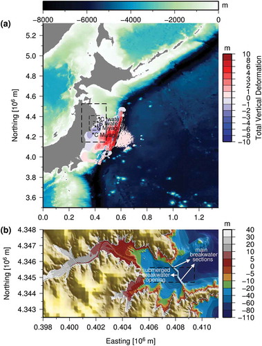
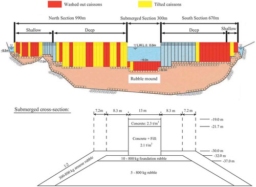
During the 2011 Tohoku-oki Earthquake Tsunami, the wave motion on and over the structure induced failure of the breakwater caissons, causing them to either slide out or lean out of position. A schematic of the breakwater is shown in Figure 4 where caissons are marked red indicating failure. Despite its failure, survey results of water marks by TTJS (Mori and Takahashi, 2012) indicate that the inundation levels were considerably lower within Kamaishi Bay, compared to levels at adjacent Ryoishi Bay where an offshore tsunami breakwater was not present. Previous numerical studies have also indicated that the breakwater likely reduced the tsunami heights into the bay by 25–40% (Mori, Yoneyama, and Pringle, 2015) and mean maximum inundation depths by 55% (Arikawa and Oie, 2015).

Figure 4. Sketch of Kamaishi Bay breakwater with the damaged caissons shaded red and yellow. Front on view and cross-section of the submerged breakwater opening; adapted from Arikawa et al. (2012).

3.2. Bathymetry Data and Computational Meshes

3.2.1. 2DH NSWE Data and Mesh

In all the simulations bathymetry and topography data from Kotani, Imamura, and Shuto (1998) with five levels of resolution (Figure 3), 1350, 450, 150, 50, and 10m are used (the computational grid sizes are set equal to the bathymetric resolution). The data from the first four mesh layers were created in the old Tokyo datum geodetic system with the origin point at UTM longitude and latitude. A total of 500 km was added onto the easting coordinate to avoid negative numbers. To generate the 10-m mesh, bathymetry from the 50-m data set was combined with 0.2 arc-second (5 m) mesh Digital Elevation Measurement topography data (Geospatial Information Authority of Japan, 2009). All ground levels are given in T.P (=L.W.L. + 0.86 m), the mean sea level in Tokyo Bay.

Figure 5. Time series of surface elevation (T.P. m) at the four GPS buoys operated by PARIa2011 that are closest to Kamaishi Bay during the 2011 Tohoku-oki Earthquake Tsunami. Comparison of 2CLOWNS-3D simulation results using the Satake v8.0 kinematic source model (Satake et al., 2013) with observations.

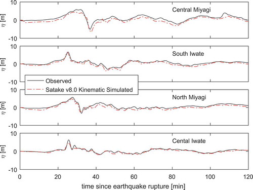
Figure 6. Filled contour plot of the maximum calculated free surfaces, η_max (in T.P. m) from the 2CLOWNS-3D simulation on the 2DH NSWE 10 m mesh. Filled circles indicate TTJS survey measurements (Mori and Takahashi, 2012). The dashed rectangle indicates the location of 3D RANS mesh.

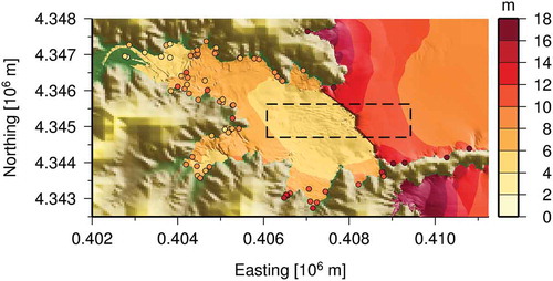
Figure 7. Comparison of run-up/inundation heights, η_max from the 2CLOWNS-3D and 2DH NSWE model simulations versus TTJS survey measurements (Mori and Takahashi, 2012). Left plot shows the comparison in bays surrounding Kamaishi (Toni, Ryoishi, and Otsuchi), while the right plot shows the comparison inside Kamaishi Bay. The geometric mean and the geometric standard deviation (Aida, 1978) between simulated and measured η_max are also indicated.

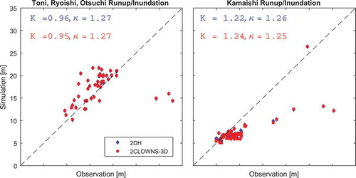
Figure 8. Time series of the horizontal volume flux per unit width (averaged in the north–south direction) over the submerged opening of the large-scale offshore breakwater during the 2DH NSWE and 2CLOWNS-3D simulations. Two 2DH NSWE simulations are conducted where;  = 0 and,  = 0.5.

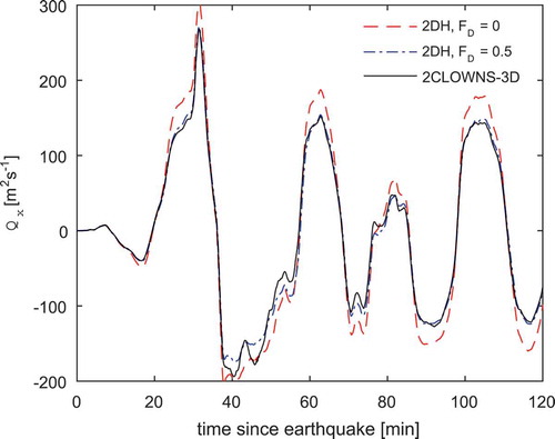
Figure 9. Time series of the forces on the submerged caissons for the 2CLOWNS-3D and 2DH NSWE simulations. (a) Magnitude of drag force per unit width, , (b) magnitude of overturning moment per unit width about the caisson heel, . The shaded areas indicate the range of forces over the width of the submerged breakwater opening while lines indicate the mean value.

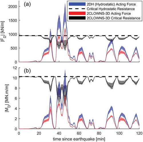
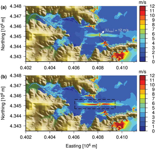
Figure 10. Filled contour plot of the maximum calculated magnitudes of the depth-averaged velocities, during model simulations on the 10 m 2DH NSWE mesh. (a) 2DH NSWE, (b) 2CLOWNS-3D dashed black rectangle indicates the extent of the 3D RANS domain.

Roughness data in the form of Manning’s friction coefficients are included in the data set that varies throughout the domain depending on the land use. Manning’s is equal to 0.025 sm in offshore areas, 0.020 sm over farmland, 0.030 sm over forestland, and 0.040 sm in populated areas as described in Kotani, Imamura, and Shuto (1998). Sub-grid scale levee crest heights are also contained in the data set and these are set on the cell boundaries using Equation (4) to calculate the volume fluxes here.

3.2.2. 3D RANS Mesh

The same bathymetry/topography data from the 2DH NSWE 10 m mesh layer are used to form the 3D RANS mesh in a localized region around the breakwater opening as shown in Figure 3(b). The extent of the domain and grid sizes is estimated based on the experimental studies of Fujima, Masamura, and Goto (2002) and Fujima (2006) (denoted FJexp) where a long sinusoidal tsunami-like wave was propagated through a breakwater opening (and over a submerged structure in Fujima (2006)). The setup in these experiments is directly comparable to the current scenario because their prototype scale of 1/200 implies a water depth,  m. This is equivalent to the representative depth in the vicinity of the Kamaishi Bay breakwater. In FJexp, the domain was chosen to be square-shaped with lengths equal to three times the width of the breakwater opening. The width of the Kamaishi Bay breakwater opening is approximately 310 m. Thus, the width (north–south direction) of the domain is selected to be 930 m in this study centered on y = 4345,165 m northing. The length (east–west direction) scaling was chosen to include a comparison of the Froude numbers, of the waveforms between FJexp and the one near Kamaishi Bay breakwater so that the length of the turbulent jet structure that we wish to capture in the 3D RANS model does not extend beyond the domain.

Making the linear long wave assumption implies , the dimensionless wave height. The equivalent prototype wave height in FJexp is  m and the leading positive wave measured at South Iwate (the offshore buoy closest to Kamaishi Bay) in  m has  = 6.7 m (Figure 5). at the breakwater ( m) can be estimated using Green’s law to be  m. This implies that is 2.3 times as large in the current scenario in comparison to FJexp for the inundating flow. Hence, the length of the domain onshore of the breakwater should in fact be approximately (3)(2.3) = 6.9 times the width of the breakwater opening, equivalent to roughly 2100 m. Similarly for the maximum drawback flow, we take  −3.0 m recorded at South Iwate at 46 min after the earthquake rupture (Figure 5). This gives  −4.1 m at the breakwater and thus the length of the domain offshore of the breakwater should roughly be the same as FJexp, i.e. three times the width of the breakwater, 930 m. x = 408,150 m easting is taken as the center of breakwater where we measure the offshore and onshore distances.

The scaling in FJexp implies that the horizontal resolution on the prototype scale was set to 10 m, the same resolution as the finest 2DH NSWE mesh layer in this study. Hence, 10 m horizontal resolution is also adopted for the 3D RANS mesh. The vertical grid size () in FJexp was half that at 5 m. However, since is 2.3 times the size for the inundation flow in our setup, we reduce to 2.2 m.

In addition, to justify that coupling for this specific scenario is reasonable, appropriate dimensionless variables introduced in Pringle, Yoneyama, and Mori (2016) can be calculated and compared with the suggested applicable range. Following Chan and Philip (2012), a crude estimate of the slope from between South Iwate wave buoy and Kamaishi Bay is given as , where the buoy is at an offshore depth of  m. The peak wave amplitude was recorded as  m ( = 0.033) at this location, and Chan and Philip (2012) approximate the effective wave length to be  km. The dimensionless slope parameter is thus . Pringle, Yoneyama, and Mori (2016) suggest that if and , then coupling can occur anywhere on a sloping beach even close to the shoreline, and errors associated with coupling will be less than 1%, respectively. In this case, and , inferring that coupling can reliably take place in small depths close to the coast or a breakwater structure while coupling errors due to shoaling are expected to be almost negligible for this scenario.

3.3. Model Conditions

The initial water level in the simulation is set at T.P. +0.0 m. The tsunami is generated by temporal deformation of the seabed . The tsunami source used to prescribe the vertical deformation used in this study is based on the Satake v8.0 model (Satake et al., 2013) where a filled contour plot of the total vertical deformation of the seabed is shown in Figure 3(a). Satake v8.0 is inversion based, consisting of 55 sub-faults each of sizes 50 × 50 km except for near trench sub-faults which are 50 × 25 km. The total slip varies from 0 to 69 m and the temporal variation of the slip for each sub-fault is specified every 30 s for a total of 5 min. The Okada (1985) rectangular fault model is used to calculate the actual deformations of the seabed. Horizontal displacements are also considered using the Tanioka and Satake (1996) method which become important in regions of large slopes and when the horizontal displacements are significant in comparison to vertical deformations. As demonstrated in Satake et al. (2013) and Goda et al. (2014), this was the case for the 2011 Tohoku-oki Earthquake Tsunami where the use of the Tanioka and Satake (1996) method increases the seabed deformation quite substantially. Combined with temporal deformation of the seabed (termed “kinematic” source as opposed to the commonly used static instantaneous deformation assumption), the Satake v8.0 model generates very robust agreements with wave buoy observations, among the best surveyed in Goda et al. (2014).

The tsunami is simulated for a total of 2 h from the earthquake rupture. Open boundary conditions are employed in the outermost 2DH NSWE mesh layer to reduce reflections of the tsunami wave. The nesting algorithm of 2CLOWNS-3D is employed to simulate the tsunami from the source toward Kamaishi Bay with increasing resolution. Different time steps are utilized so that the CFL condition is satisfied () in each nested layer. However, between two connecting mesh layers must be some integer multiple of each other, so the Courant number, , will be slightly lower or higher in some regions than in others. ranges between 0.19 s in the innermost 10 m 2DH NSWE mesh layer and 3.1 s in the outermost 1350 m 2DH NSWE mesh layer so that the ratio of is 2:1 between each set of consecutive mesh layers.

The time step in the 3D RANS mesh ranges from  = 0.039 to 0.097 s depending on the instantaneous , which is kept at around 0.4 for defined by the long wave speed, and 0.1 for defined by the flow velocity for stability of the SMAC algorithm. In other words, stability of the algorithm due to the flow velocity is far more critical than that based on the long wave speed. Hence, the ratio of reaches 5:1 between the 10-m 2DH NSWE mesh layer and the 3D RANS one. The rather large ratio does not appear to result in any adverse effects on the simulation. Concerning friction effects, a wall function is used in the turbulence model with uniform roughness heights specified on the seabed (1 mm), and over the rubble mound of the breakwater (10 cm). The results shown in Sections 4–6 are those obtained when using the realizable version of the model except where indicated.

Computation was performed on 2.67 GHz Intel® Xeon® 5650 Series processors using 12 OpenMP threads. The 2CLOWNS-3D simulation takes up to 5 days to complete while the 2DH NSWE simulation takes just over 1 h. For reference, the size of the computational matrix (number of cells) for each domain is (in order of increasing resolution) (1) , (2) , (3) , (4) , (5) , (3D) . In summary, a total of 3.504 million grid cells are computed in the 2DH NSWE simulation, and 4.875 million grid cells are computed in the 2CLOWNS-3D simulation.

4. Validation of Tsunami Height and Maximum Inundation Measurements

This section gives an overview of the simulation results that are measured in the 2DH NSWE mesh layers. This is to validate that the incoming tsunami wave and maximum inundation measurements are comparable to reality so that we have confidence in the wave forcings given by the source model, the 3D domain size, and two-way coupling scheme in 2CLOWNS-3D.

4.1. Free Surface Elevation Time Series

Temporal variation in the free surface elevation is shown at positions corresponding to the four Port and Airport Research Institute of Japan (2011) GPS buoys (locations are indicated in Figure 3(a)) closest to Kamaishi Bay in Figure 5. Overall, good agreement is found between the measured and simulated time series in both amplitude and phase (no shifting of the time series has been conducted which would normally be required for static instantaneous source models). In particular, the entire time series, including the leading positive wave peak amplitude, at South Iwate (the closest buoy to Kamaishi Bay), is well represented. Thus, the source model is considered suitable for the analysis of maximum inundation heights and hydrodynamic effects in Kamaishi Bay. Furthermore, our model results are in excellent agreement with the simulated results presented in Goda et al. (2014) using the same source model.

4.2. Maximum Inundation Heights

The maximum free surface levels η_max calculated during the 2CLOWNS-3D simulation are plotted in Figure 6 on the 2DH NSWE 10 m mesh. Free surface elevations between 10 and 14 m are calculated just offshore of the breakwater. Just onshore of the breakwater η_max is significantly reduced to 5–6 m. Thereafter, η_max is amplified by the topography. η_max becomes largest in the southern part of Kamaishi Bay, while η_max remains relatively small and attenuated by the seawalls, levees, and macro-roughness in the populated regions; Kamaishi City situated in the northeast part of Kamaishi Bay and Heita situated in the region south of this. This general behavior is in good agreement with other simulations that assume an undamaged offshore breakwater similar to this study (Mori, Yoneyama, and Pringle, 2015; Ozer Sozdinler et al., 2015; Bricker, 2013; Takahashi et al., 2011).

Comparisons with the TTJS tide-corrected survey measurements (Mori and Takahashi, 2012) are conducted. Figure 6 gives a spatial overview of the comparison where the filled circles indicate the measured maximum run-up and inundation heights at those locations. Figure 7 plots simulated versus measured run-up and inundation heights (η_max on land) where data are separated between those in the bays surrounding Kamaishi (Toni, Ryoishi, and Otsuchi) and those inside Kamaishi Bay. Goodness of fit between simulation and survey measurements is indicated by the geometric mean, (=1 perfect fit, 1 overestimation, 1 underestimation), and the geometric standard deviation, as defined by Aida (1978). It is recommended that and (Aida, 1978). In the surrounding bays,  = 0.95 and  = 1.27, indicating slight overestimation in η_max by the simulation. Three outlier locations significantly underestimate the run-up, mainly due to the inadequacy in resolving locally steep topography. Without any calibration, this can be considered a robust result because and are within the recommended limits. On the other hand, inside Kamaishi Bay,  = 1.24 and  = 1.25, indicating a relatively large overall underestimation in η_max. However, this is expected because an undamaged rigid breakwater is assumed in this study, while the breakwater was actually damaged during the tsunami, probably during the peak inundating flow given that the dislodged caissons were found on the onshore side of the breakwater (Arikawa and Oie, 2015; Arikawa et al., 2012). It has been previously shown that the measured inundation depths were approximately 21% greater than those simulated using an undamaged breakwater (Arikawa and Oie, 2015). Thus, if  = 1.24 is assumed to represent a 24% underestimation in η_max, then the accuracy of our simulation can be considered adequate.

5. Comparisons between 2DH NSWE and 2CLOWNS-3D Simulations

This section compares results from the 2DH NSWE and 2CLOWNS-3D simulations to check both large-scale effects on inundation and local effects in the vicinity of the submerged breakwater opening. The aim is to identify where the 2DH NSWE model is adequate and what information can be gained by using a 3D RANS model around the breakwater.

5.1. Maximum Inundation Heights

Comparisons of η_max between the 2CLOWNS-3D and 2DH NSWE simulations are illustrated in Figure 7. Overall, η_max is only slightly affected by the introduction of the 3D RANS model with very small changes in and compared with the 2DH NSWE simulation. In particular, is increased from 1.22 to 1.24 inside Kamaishi Bay, indicating a minor decrease in tsunami heights. This could be due to the turbulent viscosity in the 3D model taking slightly more energy out of the flow than in the 2DH NSWE model, hinting that small-scale 3D circulation effects can be of minor importance to large-scale effects. However, in general, this result demonstrates that 2DH NSWE models are typically suitable to analyze large-scale inundation effects even when a large-scale offshore breakwater shielding the bay mouth is present. Furthermore, the results imply that coupling the 3D RANS and 2DH NSWE models in 2CLOWNS-3D does not introduce significant boundary effects that might undermine the simulation due to issues with the coupling scheme and/or domain size. In addition, when using the standard model, the turbulent viscosity becomes much larger than that when the realizable version is utilized (see Section 6.2.3). The effect of the standard version is to decrease the tsunami heights so that  = 1.28 and  = 1.25 inside Kamaishi Bay. Nevertheless, this effect is fairly small in comparison to the consideration of the momentum loss due to dispersion at the breakwater opening in the 2DH NSWE model discussed in Section 5.2.

5.2. Volume Fluxes Through Submerged Breakwater Opening

It was found that in order for the 2DH NSWE model to almost match the 3D RANS model in terms of η_max, a nonzero value of for momentum loss due to dispersion over the submerged caissons is required. Calibration of a 2DH NSWE model with a physical experiment of tsunami flow through a large-scale breakwater model with a submerged breakwater opening has been previously conducted (Goto and Sato, 1993). In Goto and Sato (1993), it was shown that setting at the computational cells that represent the submerged caissons (and zero everywhere else) gave the best results in terms of offshore and onshore free surface levels. Rather, surprisingly, utilizing in this study also led to strong agreement in the time series of the average horizontal volume flux per unit width at the submerged caissons between the 2DH NSWE and 2CLOWNS-3D simulations (Figure 8). In contrast, a 2DH NSWE simulation with everywhere results in 13% greater volume fluxes through the breakwater during the peak inundating flow ( min) than when setting at the submerged caissons. Thus, setting is a necessary and suitable value to use at the submerged opening of a large-scale offshore breakwater in a 2DH NSWE simulation. Furthermore, the result indirectly indicates that the 3D RANS model can simulate the dispersive flow over the breakwater adequately as the exact same value for found through calibration with a physical experiment was used.

5.3. Hydrodynamic Forces on Submerged Breakwater Caissons

The hydrodynamic forces on the caissons are estimated in this section. Comparisons with critical values of the drag force, , and overturning moment about the caisson heel, , are evaluated. is determined by summing the pressures on the computational cells normal to the caisson in the horizontal direction multiplied by the surface area. can be found by summing the multiple of each of those forces by the vertical distance to the caisson heel. To determine the critical values for comparison, the caisson weight and lift force, , are required. The caisson weight is calculated from the dimensions and densities shown in Figure 4. To get , the pressures on the computational cells normal to the caisson in the vertical direction multiplied by the surface area are summed. Since the rubble mound is simulated as an impermeable layer in this study, it is assumed that the pressure acting underneath the caissons is the average of the pressures at the cells located either side of the caisson just above the rubble mound. The critical resistance friction force, F_Dcrit, is calculated by

(17)

where the coefficient of friction between the caisson and rubble mound, , is taken to be 0.6 (Tanimoto and Takahashi, 1994), and is the mass of the concrete caisson. Similarly, the critical resisting overturning moment, M_Dcrit is equal to

(18)

where is the distance from the center of mass of the caisson to its heel.

Time series of the magnitudes of the acting forces, and , and the critical resistance forces, and , are plotted in Figure 9 per unit width. The mean values with maximum and minimum bounds of the forces over the length of the submerged breakwater opening during both 2CLOWNS-3D and 2DH NSWE simulations are shown. Interestingly, the maximum values of and occur at 40.6 and 46.0 min during the peak drawback flow rather than the peak inundating flow. However, the caissons that were washed out were distributed onshore of the breakwater (Arikawa and Oie, 2015; Arikawa et al., 2012) indicating that failure most likely occurred during the peak inundating flow. According to the 2CLOWNS-3D simulation, the drag force may have just exceeded the critical resistance force for some caissons during the inundating flow, but the overturning moment is significantly below the critical resisting moment. In addition to the drag force, joint flow scour of the rubble mound due to extremely the fast flow (Takahashi et al., 2011; Arikawa et al., 2012) and jet impingement on the slope and armor units (Mitsui et al., 2014) have been identified to undermine caisson stability helping them to slide and tilt. A combination of drag force and joint flow scour are the likely contributors to the failure of the submerged caissons. If the caissons had not failed during the peak inundating flow, it is likely that they would have failed during the stronger drawback flow.

In the 2CLOWNS-3D simulation during peak flow events, the critical resistance forces decrease as the lift force increases. The increase in lift forces is because the pressure on the top of the caissons become significantly less than the hydrostatic pressure (see Section 6.1 for more detail). Furthermore, the pressure forces acting on the front and back faces of the caissons are slightly greater than hydrostatic. It is a combination of these effects that can make a non-hydrostatic analysis significantly different to a hydrostatic one. An interesting result of this study is that the differences between the free surface elevations near the front and back faces of the submerged caissons become so large in the 2DH NSWE model that the hydrostatic drag force predicted by that model far exceeds the drag force simulated using the 3D RANS model (Figure 9). This is because the 2DH NSWE model needs to balance the horizontal momentum without non-hydrostatic pressure or vertical accelerations and thus relies totally on the free surface difference (hydrostatic pressure gradient) to achieve this. As a result, the free surface level very close to the submerged caissons becomes wildly inaccurate, even though free surfaces slightly further from the caissons are not significantly different to those in the 3D RANS model. Interestingly, comparing acting forces simulated by the 2DH NSWE model with the critical hydrostatic resistance forces results in a similar conclusion on caisson stability to the one we reached with the 2CLOWNS-3D result, i.e. the relative balance of the acting and resisting forces calculated by the 2DH NSWE and 2CLOWNS-3D simulations are similar. With that being said, both the acting and critical resistance forces are approximately 65% larger in the 2DH NSWE simulation during the peak drawback flow in an absolute sense.

5.4. Depth-Averaged Velocities

The maximum calculated magnitudes of the depth-averaged velocities, , are shown in Figure 10 for both the 2DH NSWE and 2CLOWNS-3D simulations. Far outside of the 3D domain, no noticeable difference in the velocities arises due to the use of the RANS equations around the breakwater opening. On the other hand, the magnitude and length of the jet structure are noticeably greater in the 2CLOWNS-3D simulation: the magnitude of the centerline velocity exceeds 10 m/s up to roughly 1 km from the submerged caissons for both the inundating and drawback flows; and the edge of the inundating jet structure is located approximately a further 700 m downstream compared to the 2DH NSWE simulation. In the 2DH NSWE simulation, maximum centerline velocities are equal to approximately 6–7 m/s and quickly diffuse out. In addition, is very large, averaging 12 m/s, at the submerged breakwater opening in the 2DH NSWE simulation (indicated in Figure 10(a)). in the 2CLOWNS-3D simulation at the breakwater opening is more modest, averaging 9.7 m/s. This can be attributed to the fact that the free surface rapidly drops in the 2DH NSWE simulation over the submerged caissons (see also Section 5.3) resulting in a small water depth and therefore a very high depth-averaged velocity.

Since the volume flux through the submerged breakwater opening is roughly the same between the two simulations (Figure 8), generally larger values of concentrated in the centerline of the jet when using the 3D RANS equations indicate differences to the horizontal spreading rate of the jet. Indeed, the jet is shown to be more diffusive in the north–south directions in the 2DH NSWE simulation (Figure 10). While it is plausible that part of the reason for this is the diffusive nature of the advection scheme in the 2DH NSWE model, this reason alone cannot account for such large disparity. Besides, the 3D RANS model includes turbulent mixing terms which are ignored by the 2DH NSWE model. The majority of the difference instead must be related to the fact that significant vertical accelerations and vertical growth of the jet occur in the 3D RANS model. The 2DH NSWE model, due to its single-layer assumption, only allows for the jet to grow in the horizontal direction assuming no vertical variation of the horizontal velocity. Consider that the flow becomes essentially isotropic in three-dimensions as it flows over the submerged caissons growing in both horizontal and vertical directions like a wall-jet (see Section 6.2). Under these conditions, the 2DH NSWE model will be insufficient to correctly reproduce the flow structure.

5.5. Bed Shear Stresses

The fast flow onshore of the breakwater can cause large bed shear stresses leading to significant sediment transport in the harbor. This could induce unwanted erosion and deposition of sediment which can lead to instability of coastal structures.

To estimate the bed shear stress, in this study, the quadratic form is used:

(19)

where is a dimensionless coefficient, and is the magnitude of the horizontal velocity measured in the computational cell just above the bed. The density of the sea water, , is assumed to be 1025 kg/m³, and a constant value of  = 0.0025 is adopted. The quadratic form with a constant value of is used to make comparisons between the 2DH NSWE and 3D RANS models straightforward. Note that in the case of the 2DH NSWE model, . is converted to a dimensionless form to represent the ease at which sediment transport is induced:

(20)

where is the density of the sediment and is taken to be 2650 kg/m³, and is the median grain diameter taken to be 1 mm on the seabed and 10 cm over the rubble mound.

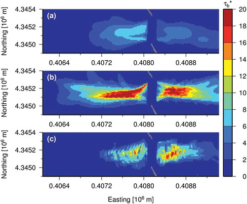
Figure 11 plots the maximum calculated in the area around the breakwater opening from the 2DH NSWE and 2CLOWNS-3D simulations. A case where is used instead of from the 2CLOWNS-3D simulation is included to illustrate the significance of the vertical variation of the velocities. using is up to 310% larger in the 3D RANS model than the 2DH NSWE model which is to be expected since is approximately 60–70% larger (Figure 10) within the jet structure. using from the 2CLOWNS-3D simulation is larger than 16 up to 1 km from the submerged caissons and is greater than 1 up to 2 km from the submerged caissons. However, using to calculate suggests that values greater than 1 are primarily focused within a 1-km range from the submerged caissons, thus erosion would have likely occurred in this region. Furthermore, is larger on the offshore side of the breakwater using , while is larger on the coastal side using from the 2CLOWNS-3D simulations. Thus, the velocities near the seabed become larger during the peak drawback flow than during the peak inundating flow (see also Section 6.1). Our simulations suggest that the armor of the rubble mound would have been relatively unaffected during the tsunami. However, jet overflow and impingement on the slope and armor blocks, which is likely to cause failure (Mitsui et al., 2014), are not explicitly simulated.

Figure 11. Comparisons of the maximum dimensionless bed shear stress, , around the breakwater opening assuming a uniform grain size,  mm, on the seabed and  cm over the rubble mound. (a) 2DH NSWE simulation, (b) 2CLOWNS-3D simulation using depth-averaged velocity, (c) 2CLOWNS-3D simulation using near-bed velocity. The main breakwater sections are plotted in gray.

6. Analysis of the 3D Flow Hydrodynamics around the Breakwater

This section investigates the 3D hydrodynamics of the flow around the offshore breakwater resulting from the 2CLOWNS-3D simulation to examine reasons for the disparity in the depth-averaged velocities and forces acting on the caissons between the 2DH NSWE simulation and evaluate the ability of 2CLOWNS-3D to adequately model the 3D effects. First, the vertical distribution of the pressure and velocity fields in the 3D domain is discussed. Second, we analyze the jet structure during the peak inundating tsunami flow emanating from the submerged breakwater opening by approximating it as a transient slender wall jet.

6.1. Vertical Distribution of the Pressure and Velocity Fields

In Section 5, it has been shown that momentum dispersion effects and the non-hydrostatic pressures become large causing an increase in lift forces over the submerged caissons. Between 2DH NSWE and the 3D RANS models, the horizontal distribution of varies considerably. Vertical variations of the velocities in the 3D RANS model may also be significant. This section describes the distribution of the hydrodynamics in the plane during from the 2CLOWNS-3D simulation. Figure 12 plots the velocity field vectors and dynamic pressure (difference from hydrostatic pressure) colormap along the y = 4345,175 m northing cross-section at two different times corresponding to the time of peak inundating ( = 31.6 min) and drawback ( = 40.5 min) flow.

Figure 12. Velocity field vectors and dynamic pressure (difference from hydrostatic) colormap along the y = 4345,175 m northing cross-section inside the 3D RANS domain at t = 31.6 min (peak inundating flow) and t = 40.5 min (peak drawback) after the earthquake rupture. The left-hand side plots the entire 3D RANS model domain while the right-hand side zooms in closer to the breakwater.

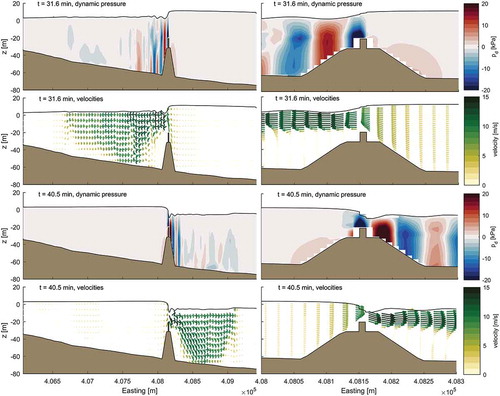
During both the peak inundating and drawback flow, and the velocities are fairly small at both east and west boundaries (left hand side of Figure 12). Therefore, in general, the shallow water flow requirement of hydrostatic pressure and vertically uniform flow at the boundary for accurate coupling between the 2DH NSWE and 3D RANS model appear to be largely satisfied throughout the simulation. Although in the design of the 3D RANS mesh it was not anticipated that the drawback would be as strong or even stronger (Figure 9) than the inundating flow, so the mesh was made shorter in the offshore direction. Nevertheless, there is a good agreement in the time series of the volume fluxes through the submerged breakwater opening between the 2DH NSWE and 2CLOWNS-3D model simulations (Figure 8), thus any negative impact at the boundary can be considered relatively small. Furthermore, the boundary condition that allows for an arbitrary vertical distribution of the horizontal velocities used in this study should enable such vorticities in the 3D RANS model to cross through the model coupling interface (Fujima, Masamura, and Goto, 2002).

As the flow encounters the rubble mound and submerged caisson, the flow structure rapidly changes. First, the horizontal velocity starts to become greater near the free surface than near the seabed as it approaches the submerged caisson. Over the caisson, the horizontal velocity becomes as large as 12 m/s for both inundating and drawback flow at the grid points just above the caisson. The flow downstream of the caisson on the rubble mound is strongly vertically nonuniform due to the shielding effects of the caisson and vertically uniform flow is not recovered until around 1–2 km downstream from the submerged breakwater opening. Furthermore, there are undulations present in the free surface and the vertical velocity field in this region. The dynamic pressure is shown to become slightly positive near the seabed as the wave flows up the rubble mound. Over the submerged caisson, becomes strongly negative (reaching −38 kPa during peak inundating flow and −67 kPa during peak drawback). Thereafter, is positive just downstream of the submerged caisson above the rubble mound before changing back to a negative value near the edge of rubble mound. As also suggested in plots of the bed shear stress (Figure 11), the velocities appear to be directed down toward the seabed at a steeper angle and have a higher magnitude during the peak drawback flow on the offshore side of the breakwater than during the peak inundating flow on the coastal side.

The explanation for the observations described above and shown in Figure 12 is as follows. As the flow encounters the rubble mound, which is a steep 2:1 slope, vertical accelerations are significant especially near the seabed, causing and the vertical velocities to become large. At the caisson, there is a rapid change in the momentum flux which requires a large pressure force imbalance to match it, i.e. the pressure over the caisson must drop considerably. The pressure drop is achieved by the formation of a hydraulic jump where the pressure becomes less than hydrostatic and the free surface drops rapidly (although much less rapidly than predicted by the 2DH NSWE model). Downstream of the caisson, a jet structure develops where the horizontal velocities are very small at depths below the edge of the jet but are larger than 10 m/s within the jet. The horizontal velocities within the jet structure are also fairly uniform over the depth. This peak inundating jet structure is the subject of Section 6.2 where its behavior is analyzed in detail. The reason for larger velocities along the seabed during the peak drawback flow could be because it must interact with onshore-directed flow arriving from offshore focusing the flow down toward to the seabed.

6.2. Analysis of the Onshore Directed Large-Scale Jet Structure

The aim of this section is to examine the basic behavior of the onshore-directed large-scale jet structure and attempt to validate the flow in the 3D RANS model during the 2CLOWNS-3D simulation versus empirical measures of maximum velocity decay and half-width growth for a transient wall jet. Furthermore, as the wall jet is a highly turbulent phenomenon, it allows us to evaluate the performance of the two forms of the turbulence model.

6.2.1. Overview of Slender Wall Jet Characteristics

The canonical schematic of a slender wall jet in the current setting is shown in Figure 13. The free surface is approximated as a wall (although with the complication that the velocity at the free surface does not go to zero like a true wall), and the jet is free to grow in the horizontal directions and vertically downward until it reaches the seabed. The slenderness refers to the fact that the width of the opening,  = 310 m, is much larger than the height,  25 m. For further reference, this implies the ratio  12.5. In this study, we make comparisons with empirical measurements of decay of the maximum (centerline) longitudinal velocity downstream from submerged breakwater opening, and growth of the longitudinal velocity half-width (the transverse distance from the maximum velocity position where the velocity becomes half of the maximum for both vertical, denoted , and horizontal, denoted , directions).

Figure 13. Schematic of the canonical wall jet under the current setting of flow through the submerged breakwater opening. The three regions of decay of the maximum (centerline) longitudinal velocity, , are indicated along with the approximate distances from the submerged breakwater opening that the regions extend to (based on a slenderness ratio ).

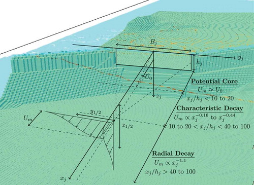
For 3D jets, there are three distinct regions with different rates of decay of ; potential core, characteristic decay, and radial decay regions (Sforza and Herbst, 1970) (Figure 13). In the potential core region, remains equal or close to that of the jet exit velocity, . This region extends up to a distance from the opening for the slenderness ratio we are concerned with () (Sforza and Herbst, 1970). The characteristic decay region refers to decay of similar to that of a plane wall jet. However, the actual rate of decay, as well as the distance the region extends to, depends on the slenderness ratio . Based on Sforza and Herbst (1970), the rate of characteristic decay of is extending a distance from the opening when and is extending a distance from the opening when . The decay rate of in the radial decay region (extending from the characteristic decay region to the edge of the jet) has been found to be similar to that of a round jet decay rate () independent of (Sforza and Herbst, 1970).

Half-width growths in the vertical direction, , are found to be independent of and are everywhere in the jet (Sforza and Herbst, 1970). This is roughly 20% smaller than growth rates of plane (Schwarz and Cosart, 1961) and round wall jets (Bakke, 1957). Half-width growth rates in the horizontal directions are however not characterizable by a single power coefficient. Initially, near the jet, opening growth of is approximately stagnant for and slightly negative for . Further, downstream the growth rate rapidly increases becoming independent of (Sforza and Herbst, 1970), estimated from plots to be .

6.2.2. Turbulent Modeling of the Jet

First, it should be mentioned that the assumption has been made in Equation (6) that the turbulence is directionally isotropic. Usually in oceanic flows, anisotropic turbulence is assumed given the vastly different length scales, in addition to the predominantly vertical effects of the oceanic surface boundary layer, internal wave breaking, Richardson instability, and double diffusion, e.g. as found in the KPP model (Large, McWilliams, and Doney, 1994). However, in this case, the flow through the submerged breakwater opening and that a good distance downstream completely overwhelms the surface boundary layer and other comparatively small effects such as double diffusion. Here, the mixing in vertical and horizontal directions are both large and the isotropic assumption is considered reasonable in the opinion of the authors (e.g. as used for modeling classical jet phenomena).

Without going into great detail, the differences of the standard and realizable models are highlighted. The equation for is identical between the models. The difference between the equations is the source term (Shih et al., 1995). In the standard model, the Reynolds stresses themselves appear in the source term, while in the realizable model, the source term is directly related instead to the mean strain rate, (). Since generally behaves better than Reynolds stresses numerically, the realizable equation can be described as more robust (Shih et al., 1995). A quantitatively more obvious difference between the models revolves around the expression for :

(21)

 = 0.09 found for boundary layer flows in the inertial sublayer is adopted as a constant in the standard model. However, for a large mean strain rate ( 3.7) in homogeneous shear flows,  = 0.05 (Shih et al., 1995). Using a constant value,  = 0.09, can cause the Reynolds stresses to become negative for  3.7 and the model unrealizable. Modeling as a variable related to the mean strain rate is thus the main remedy that the realizable model proposes. Indeed, improving the modeling of free shear flows such as a round jet where the standard model overpredicts the spreading rate was one of the motivations for development of the realizable model. Thus, we can expect the realizable model to perform better than the standard one in the current scenario where the mean strain rate becomes large.

6.2.3. Numerical Results of Jet Characteristics

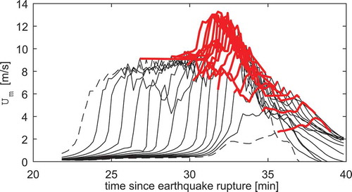
First, in order to analyze the jet characteristics, the transient flow needs to be converted into an equivalent steady flow. To achieve this, time averaging is performed over the interval where is in the upper 20th percentile of itself between the 21.7 and 40-min interval for each longitudinal coordinate downstream of the breakwater. As plotted in Figure 14, the upper 20th percentile of (red lines) is shown to encompass the time interval where there is a noticeable peak in for each individual location. Thus, the upper 20th percentile can be said to correspond to the time interval that captures the peak inundating jet structure over which time averaging can be performed.

Figure 14. Time series of maximum (centerline) longitudinal velocities, at various longitudinal positions downstream from the submerged breakwater opening for the realizable model simulation. The dashed black lines are the time series at and , and the solid blacks lines are those in the range . Time averaging for analysis of jet characteristics is performed over the time interval where is in the upper 20th percentile (indicated by the red lines) for the plotted interval at each longitudinal position.

The decay of versus in our numerical experiments is shown in Figure 15(a) for both the standard and realizable models. Three linear best fit lines of the data for each region of decay (potential core, characteristic decay, and radial decay) are approximated using a least squares fit. The Shape Language Modeling engine (https://www.mathworks.com/matlabcentral/fileexchange/24443-slm-shape-language-modeling?focused=7538987&tab=function) is used to find the start and end points of each line/region by employing the “free knot” setting (with four knots) and a polynomial of degree one. The edge of the jet is set at , beyond which a sudden drop-off in velocity is noticeable because the jet did not have enough time to fully develop. The three regions of decay are relatively well defined in both models. The length of each region of decay is longer in the realizable model. Both models satisfy the requirement that the rate of characteristic decay region should be between −0.16 and −0.44 for  = 12.5. However, only the realizable model satisfies the observation that the radial decay region should begin somewhere between (Sforza and Herbst, 1970). Furthermore, the realizable model gives a decay rate of −1.21 fairly close to the expected rate of −1.1. The standard model gives a larger decay rate (−1.86). However, the rate of decay in the radial region can not be exactly defined since it fluctuates based on the choice of the edge of the jet. Although varying the edge of the jet between gives an average decay rate of −1.91 (SD = 0.35) and −1.25 (SD = 0.39) for the standard and realizable models, respectively, indicating that the realizable model does appear to more adequately approximate the longitudinal decay of overall.

Figure 15. (a) Decay of the maximum (centerline) longitudinal velocity, , of the transient wall-jet with distance downstream of the breakwater; (b) growth of the half-width of the transient wall-jet in the horizontal, , , and vertical planes. Left plots: Standard model; Right plots: realizable model; Regions I: potential core; II: characteristic decay; III: radial decay.

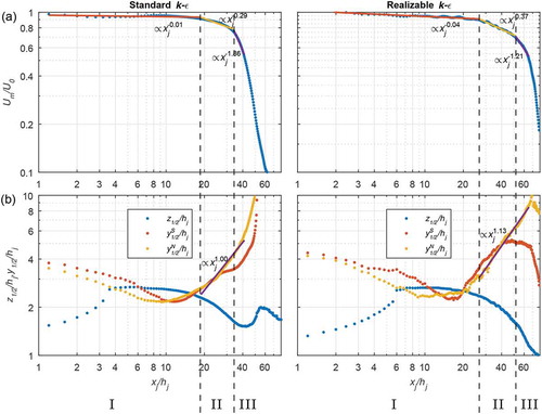
The growth of and versus is plotted in Figure 15(b). Here, and refer to the horizontal half-widths in the south and north directions, respectively. Although it is expected that the growth of will conform to a power law for both models, the growth rate of rapidly accelerates before interaction with the seabed at . Note however that the growth here is taking place in the potential core region and is thus somewhat unreliable. Furthermore, in our example, the growth of should be complicated by the presence of the seabed and due to the fact that velocity at the free surface does not go to zero like a true wall. Comparatively, develops slower for the realizable model than the standard one. The basic pattern of growth of is replicated by both models; in an initial region, actually decreases before a sharp increase in growth beyond approximately from or before the transition into the characteristic decay region. The growth of from the characteristic decay region follows a power law quite reliably until the edge of the jet particularly in the realizable model (), slightly below the growth rate estimate of 1.25 from physical experiments.

The characteristics of the jet when using the realizable model appear to be more reasonable in comparison with the empirical data than the standard model. Figure 16(a) demonstrates how the maximum calculated turbulent viscosities, , along the centerline of the jet are much larger in the standard model reaching a maximum of 15.4 m²/s at which is close to the position of the jet edge determined in Figure 15. In contrast, gradually climbs up to a maximum of 4.9 m²/s near the edge of the domain in the realizable model. This indicates that the jet simulated by the standard model is far more viscous than that simulated by the realizable one; hence, the development of the jet occurs closer to the breakwater as demonstrated in Figure 15. Furthermore, maximum turbulent intensities in the standard model consistently exceed 100% intensity and reach a maximum of approximately 300% (Figure 16(a)). Such large values of seem entirely unreasonable. In contrast, in the middle section between , in the realizable model ranges between 11% and 19%. Also, spikes to around 100% at positions closer to the breakwater around , and is increased up to approximately 50% further downstream beyond . From our observations, these increases in appear to be controlled by the effects of bed friction. Close to the breakwater, interaction between the jet flow and the rubble mound occurs. Further downstream highly turbulent flow generated by the interaction of the jet with the seabed is directed up toward the free surface and becomes entrained by the jet.

Figure 16. (a) Maximum values of the turbulent viscosity, , and turbulent intensity, , along the centerline of the transient wall-jet with distance downstream of the breakwater comparing the standard and realizable models; (b) minimum values of the coefficient of turbulent viscosity, , along the centerline with distance downstream of the breakwater for the realizable model.

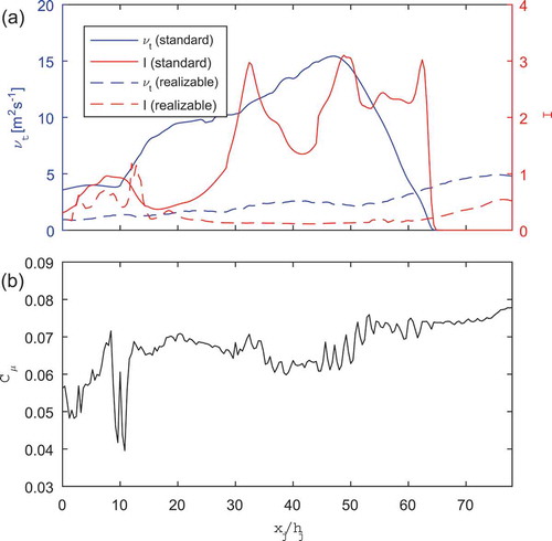
Figure 16(b) illustrates the minimum calculated values of along the centerline of the jet. The plot demonstrates how is able to stay smaller in the realizable model. As we expect during high mean strain rate flows, reduced to values smaller than 0.05 in some regions, particularly those closer to the breakwater, which also tend to correspond to areas of high . Thus, we believe that the realizable model allows for a more robust simulation of the turbulent jet structure emanating from the breakwater and should be used over the standard version under similar conditions.

7. Conclusions and Discussion

This study used a two-way coupling approach between 2DH NSWE and 3D RANS models, named 2CLOWNS-3D. The hydrodynamics of the 2011 Tohoku-oki Earthquake Tsunami on and around the submerged opening of the Kamaishi Bay large-scale offshore tsunami breakwater, where the majority of the volume flux is conveyed in and out of the bay, were analyzed. For a total of 4.875 million grid cells, the computational time for 2 h of simulation time in the 2CLOWNS-3D model is approximately 5 days using 12 OpenMP threads.

Comparisons of modeled and observed free surface elevation time histories at offshore GPS buoys show that the tsunami source model is suitable for our application. Maximum inundation and run-up heights were also compared with survey measurements and found to be relatively accurate in the bays surrounding Kamaishi but underestimated inside Kamaishi Bay. This can be explained by the damage to the breakwater caissons during the actual tsunami event, whereas the simulations in this study consider the breakwater to be a rigid structure.

2CLOWNS-3D and 2DH NSWE simulations were compared to outline the benefits of 2CLOWNS-3D, and to identify what impacts of the tsunami the 2DH model is sufficiently capable of estimating. Time series of the volume fluxes through the breakwater opening, and maximum inundation and run-up heights between 2CLOWNS-3D and 2DH NSWE simulations were shown to be only marginally different when a suitable momentum dispersion loss factor is included in the 2DH NSWE simulation at the submerged breakwater opening ( appears to be suitable for the Kamaishi offshore breakwater). This indicates that, as long as a momentum dispersion loss factor is considered, a 2DH NSWE model is suitable for inundation analysis even when a large-scale offshore breakwater shielding most of the bay mouth is present. The results also help to confirm the robustness of the 2CLOWNS-3D coupling scheme and adequacy of the 3D RANS domain size.

The drag forces on the submerged caissons were found to be more significant than the overturning moment. The resisting forces of some caissons were marginally exceeded during the peak inundating flow when failure is expected to have occurred. The most severe drag forces and overturning moment occur during the peak drawback event. Jet impingement on the slope and armor blocks, and joint flow scour of the rubble mound (not simulated in this study) also likely played an important role to undermine caisson stability. The 2DH NSWE simulation was shown to estimate approximately 65% greater peak acting and resisting forces on the submerged caissons during the maximum drawback event in comparison with the 2CLOWNS-3D simulation because of its inability to consider vertical accelerations and associated non-hydrostatic pressures.

The depth-averaged velocities are in general 60–70% larger in the center of the jet structures emanating from the submerged breakwater opening during the 2CLOWNS-3D simulation in comparison to the 2DH NSWE simulation. Furthermore, the bed shear stresses in the vicinity of the breakwater were larger in the 3D RANS model. Significant near bed velocities in the 3D RANS model, capable of erosion of seabed sediment, are generally concentrated in a region approximately 1 km from the submerged breakwater opening. Furthermore, these near bed velocities and shear stresses were found to be stronger during the peak drawback event than during the peak inundating flow. Analysis of the vertical distribution of the velocities and dynamic pressure highlights the importance of vertical accelerations around the submerged breakwater opening. Large negative values of dynamic pressure occur over the submerged caissons where a hydraulic jump occurs with a sudden drop in free surface levels. A large-scale jet structure develops downstream of the caissons with noticeably different horizontal growth rates between the 2DH NSWE and 2CLOWNS-3D simulations.

Analysis of the onshore directed large-scale jet structure was conducted with the assumption that it behaves like a 3D transient slender wall jet. Decay of the maximum (centerline) velocity and half-width growth in the horizontal direction was shown to approximately match empirical measurements. Growth in the vertical direction appears to be influenced by the effect of the seabed and the free surface (not present in a typical wall jet), and thus not easily comparable with physical experiments. In general, it was found that a realizable turbulence model performs better than the standard version. The standard model gives excessive turbulent viscosity and intensities that the realizable model was able to suppress by reducing the variable during periods of high mean strain rate.

This study demonstrates the viability of using a coupled modeling system like 2CLOWNS-3D to enable a real-scale 3D Navier–Stokes simulation of the flow in the area of interest. Placing a 3D RANS model around a large-scale offshore coastal structure allows for an in-depth analysis of the tsunami hydrodynamics, which becomes quite different from typical shallow water flow near the breakwater (e.g. large negative dynamic pressure over the caisson, and development of 3D jet structure downstream of the breakwater). This will enable the design of coastal structures like the Kamaishi Bay offshore tsunami breakwater to be improved by providing the details of real-scale hydrodynamic forces more precisely, in addition to simultaneously computing the effects of the breakwater on the coast through the two-way coupling system. Simulations that take into account porous flow and scour of the rubble mound could also be conducted. Moreover, more accurate estimates of current speeds that affect ships and port structures and bed shear stresses that induce morphological changes to the sea bed (both shown to be substantially different between 2DH NSWE and 3D RANS models up to 1–2 km from the breakwater in this study) will be valuable information for port and ship operators.

The current study uses a fairly coarse grid resolution around the breakwater structure due the requirement of a relatively large 3D domain based on the flow conditions. An improved coupled system could use more computationally and numerically efficient 3D “non-hydrostatic” models (e.g. Ma, Shi, and Kirby, 2012) to simulate the flow in Kamaishi Bay. This will allow for the 3D RANS model domain to be defined only at the breakwater structure itself, significantly reducing the domain size. Furthermore, improving the parallelization of the code using Message Passing Interface, or adopting existing codes that utilize this (e.g. Ma, Shi, and Kirby, 2012; Takase et al., 2016), in order to use many computational processors is recommended. Future work should also focus on improving the adaptability of the models (e.g. adding and dropping terms in the governing equations dynamically) and the coupling between them (e.g. dynamic movement of domain extents) to allow for increased grid resolution whilst maintaining and improving computational efficiency.

Acknowledgments

This study was made possible thanks to the financial support of the Japanese Ministry of Education, Culture, Sports, Science, and Technology (MEXT).

Disclosure statement

No potential conflict of interest was reported by the authors.

Additional information

Funding

This study was made possible thanks to the financial support of the Japanese Ministry of Education, Culture, Sports, Science, and Technology (MEXT).

References

- Aida, I. 1978. “Reliability of a Tsunami Source Model Derived from Fault Parameters.” Journal of Physics of the Earth 26 (1): 57–73. doi:10.4294/jpe1952.26.57.
- Amsden, A. A., and F. H. Harlow. 1970. “A Simplified MAC Technique for Incompressible Fluid Flow Calculations.” Journal of Computational Physics 6 (2): 322–325. doi:10.1016/0021-9991(70)90029-X.
- Arikawa, T., and T. Oie. 2015. “A Consideration Aimed at Improving the Resiliency of Protective Structures against Tsunami.” In Post-Tsunami Hazard Reconstr. Restor., edited by V. Santiago-Fandin˜o, Y. A. Kontar, and Y. Kaneda, 211–223. Cham: Springer International Publishing.
- Arikawa, T., M. Sato, K. Shimosako, I. Hasegawa, G.-S. Yeom, and T. Tomita. 2012. “Failure Mechanism of Kamaishi Breakwaters Due to the Great East Japan Earthquake Tsunami.” Coastal Engineering Proceedings 33. doi: 10.9753/icce.v33.structures.16.
- Arikawa, T., and T. Tomita. 2016. “Development of High Precision Tsunami Runup Calculation Method Based on a Hierarchical Simulation.” Journal of Disaster Research 11 (4): 639–646. doi:10.20965/jdr.2016.p0639.
- Asai, M., Y. Miyagawa, A. Muhari, and F. Imamura. 2016. “Coupled Tsunami Simulations Based on a 2D Shallow-Water Equation-Based Finite Difference Method and 3D Incompressible Smoothed Particle Hydrodynamics.” Journal of Earthquake and Tsunami 10 (4): 1–19. doi: 10.1142/S1793431116400194.
- Bakke, P. 1957. “An Experimental Investigation of a Wall Jet.” Journal of Fluid Mechanics 2 (5): 467–472. doi:10.1017/S0022112057000270.
- Bricker, J. D. 2013. “Turbulence Model Effects on VOF Analysis of Breakwater Overtopping during the 2011 Great East Japan Tsunami.” In Proceedings of the 35th IAHR World Congress, Chengdu, China.
- Chan, I.-C., and L.-F. L. Philip. 2012. “On the Runup of Long Waves on a Plane Beach.” Journal of Geophysical Research 117 (C8): C08006. doi:10.1029/2012JC007994.
- Fujima, K. 2006. “Effect of a Submerged Bay-Mouth Breakwater on Tsunami Behavior Analyzed by 2D/3D Hybrid Model Simulation.” Natural Hazards 39 (2): 179–193. doi:10.1007/s11069-006-0022-x.
- Fujima, K., K. Masamura, and C. Goto. 2002. “Development of the 2D/3D Hybrid Model for Tsunami Numerical Simulation.” Coastal Engineering Journal 44 (4): 373–397. doi:10.1142/S0578563402000615.
- Fukazawa, S., and H. Tosaka. 2014. “Seamless and Mass-Conservative Numerical Simulation of Tsunami and Inundation with Infiltration of Water into Underground.” In Proceedings of the 1st International Conference on Computational Engineering and Science for Safety and Environmental Problems., Sendai, Japan, 703–706.
- Geospatial Information Authority of Japan. 2009. 5 M Mesh Digital Elevation Measurements of Japan (JGD2000). Japan: Tsukubashi, Ibaraki Prefecture Office.
- Goda, K., P. Mai, T. Yasuda, and N. Mori. 2014. “Sensitivity of Tsunami Wave Profiles and Inundation Simulations to Earthquake Slip and Fault Geometry for the 2011 Tohoku Earthquake.” Earth, Planets and Space 66 (1): 105. doi:10.1186/1880-5981-66-105.
- Goto, C., and K. Sato. 1993. Development of Tsunami Numerical Simulation System for Sanriku Coast in Japan. Vol. 32, 3–44 (in Japanese). Yokosuka, Japan: Port and Airport Research Institute.
- Honma, H. 1940. “Coefficient of Flow Volume on Low Overflow Weir.” Proceedings of JSCE 26 (6): 635–645 (in Japanese).
- Imamura, F., and C. Goto. 1988. “Truncation Error in Numerical Simulation by the Finite Difference Method.” Coastal Engineering in Japan 31 (2): 245–263. doi:10.1080/05785634.1988.11924496.
- Imamura, F., A. C. Yalciner, and G. Ozyurt. 2006. Tsunami Modelling Manual (TUNAMI model). Technical Report.
- Kajitani, Y., S. E. Chang, and H. Tatano. 2013. “Economic Impacts of the 2011 Tohoku-Oki Earthquake and Tsunami.” Earthquake Spectra 29 (S1): 457–478. doi: 10.1193/1.4000108.
- Kihara, Naoto, Naoki Fujii, and Masafumi Matsuyama. 2012. “Three-Dimensional Sediment Transport Processes on Tsunami-Induced Topography Changes in a Harbor.” Earth, Planets and Space 64 (10): 787–797. doi: 10.5047/eps.2011.05.036.
- Kotani, M., F. Imamura, and N. Shuto. 1998. “Tsunami Runup Calculations and Damage Estimation Method Using GIS.” Proceedings of Coastal Engineering, JSCE 45: 356–360 (in Japanese).
- Large, W. G., J. C. McWilliams, and S. C. Doney. 1994. “Oceanic Vertical Mixing: A Review and A Model with A Nonlocal Boundary Layer Parameterization.” Reviews of Geophysics 32 (4): 363. doi:10.1029/94RG01872.
- Launder, B. E., and D. B. Spalding. 1974. “The Numerical Computation of Turbulent Flows.” Computer Methods in Applied Mechanics and Engineering 3 (2): 269–289. doi:10.1016/0045-7825(74)90029-2.
- Lin, P., and P. L. F. Liu. 1998. “A Numerical Study of Breaking Waves in the Surf Zone.” Journal of Fluid Mechanics 359: 239–264. doi:10.1017/S002211209700846X.
- Liu, P. L.-F., S. B. Woo, and Y.-S. Cho. 1998. Computer Programs for Tsunami Propagation and Inundation. Technical Report. Ithaca, New York: Cornell University.
- Lynett, P. J., J. Borrero, S. Son, R. Wilson, and K. Miller. 2014. “Assessment of the Tsunami-Induced Current Hazard.” Geophysical Research Letters 41 (6): 2048-2055. doi: 10.1002/2013GL058680.
- Lynett, Patrick J., Jose C. Borrero, Robert Weiss, Sangyoung Son, Dougal Greer, and Willington Renteria. 2012. “Observations and Modeling of Tsunami-Induced Currents in Ports and Harbors.” Earth and Planetary Science Letters 327–328: 68–74. doi: 10.1016/j.epsl.2012.02.002
- Ma, G., F. Shi, and J. T. Kirby. 2012. “Shock-Capturing Nonhydrostatic Model for Fully Dispersive Surface Wave Processes.” Ocean Modelling 43–44: 22–35. doi:10.1016/j.ocemod.2011.12.002.
- Mitsui, J., A. Matsumoto, M. Hanzawa, and K. Nadaoka. 2014. “Stability of Armor Units Covering Rubble Mound of Composite Breakwaters against a Steady Overflow of Tsunami.” Coastal Engineering Proceedings 34. doi: 10.9753/icce.v34.structures.34.
- Mori, N., and T. Takahashi, The 2011 Tohoku Earthquake Tsunami Joint Survey Group. 2012. Nationwide Post Event Survey and Analysis of the 2011 Earthquake Tsunami. Coastal Engineering Journal 54 (1): 1250001-1-1250001-27. doi:10.1142/S0578563412500015.
- Mori, N., N. Yoneyama, and W. J. Pringle. 2015. “Effects of the Offshore Barrier against the 2011 off the Pacific Coast of Tohoku Earthquake Tsunami and Lessons Learned.” In Post-Tsunami Hazard Reconstr. Restor., edited by V. Santiago-Fandin˜o, Y. A. Kontar, and Y. Kaneda, 121–132. Cham: Springer International Publishing.
- Nagashima, H., S. Sasaki, W. J. Pringle, and N. Yoneyama. 2015. “Numerical Assessment of Critical Locations for Tsunami Inundation.” Journal of Japan Society of Civil Engineers, Ser. B3 (Ocean Engineering) 71 (2): I 509–I 514 (in Japanese). doi: 10.2208/jscejoe.71.I_509.
- National Police Agency of Japan. 2018. “Damage Situation and Police Countermeasures.” https://www.npa.go.jp/news/other/earthquake2011/pdf/higaijokyo_e.pdf (accessed April 23, 2018).
- Okada, Y. 1985. “Surface Deformation Due to Shear and Tensile Faults in a Half-Space.” Bulletin of the Seismological Society of America 75 (4): 1135–1154.
- Ozer Sozdinler, C., A. C. Yalciner, A. Zaytsev, A. Suppasri, and F. Imamura. 2015. “Investigation of Hydrodynamic Parameters and the Effects of Breakwaters during the 2011 Great East Japan Tsunami in Kamaishi Bay.” Pure and Applied Geophysics 172 (12): 3473–3491. doi:10.1007/s00024-015-1051-8.
- Port and Airport Research Institute of Japan. 2011. “GPS Wave Buoy Measurements of the Tohoku off the Coast of the Pacific Earthquake Tsunami.” https://nowphas.mlit.go.jp/prg/pastdata/static/sub311.htm (accessed June 12, 2018).
- Pringle, W. J., and N. Yoneyama. 2013. “The Application of a Hybrid 2D/3D Numerical Tsunami Inundation-Propagation Flow Model to the 2011 off the Pacific Coast of Tohoku Earthquake Tsunami.” Journal of Japan Society of Civil Engineers, Ser. B2 (Coastal Engineering) 69 (2): I 306–I 310 (in Japanese). doi: 10.2208/kaigan.69.I_306.
- Pringle, W. J. 2016. “Two-Way Coupled Multiscale Tsunami Modelling from Generation to Coastal Zone Hydrodynamics.” PhD diss., Graduate School of Engineering, University of Kyoto. doi:10.14989/doctor.k19677.
- Pringle, W. J., N. Yoneyama, and N. Mori. 2016. “Two-Way Coupled Long Wave RANS Model: Solitary Wave Transformation and Breaking on a Plane Beach.” Coastal Engineering 114: 99–118. doi:10.1016/j.coastaleng.2016.04.011.
- Sakunaka, J., and T. Arikawa. 2012. “Research on Stability of Opening Section at Baymouth Breakwater.”Coastal Engineering Proceedings 33. doi: 10.9753/icce.v33.structures.58.
- Satake, K., Y. Fujii, T. Harada, and Y. Namegaya. 2013. “Time and Space Distribution of Coseismic Slip of the 2011 Tohoku Earthquake as Inferred from Tsunami Waveform Data.” Bulletin of the Seismological Society of America 103 (2B): 1473–1492. doi:10.1785/0120120122.
- Schwarz, W. H., and W. P. Cosart. 1961. “The Two-Dimensional Turbulent Wall-Jet.” Journal of Fluid Mechanics 10 (4): 481–495. doi:10.1017/S0022112061000299.
- Sforza, P. M., and G. Herbst. 1970. “Study of Three-Dimensional, Incompressible, Turbulent Wall Jets.” AIAA Journal 8 (2): 276–283. doi:10.2514/3.5656.
- Shih, T.-H., W. W. Liou, A. Shabbir, Z. Yang, and J. Zhu. 1995. “A New k-ε Eddy Viscosity Model for High Reynolds Number Turbulent Flows.” Computers & Fluids 24 (3): 227–238. doi:10.1016/0045-7930(94)00032-T.
- Sitanggang, K. I., and P. J. Lynett. 2010. “Multi-Scale Simulation with a Hybrid Boussinesq-RANS Hydrodynamic Model.” International Journal for Numerical Methods in Fluids 62 (9): 1013–1046. doi: 10.1002/fld.2056.
- Son, S., P. J. Lynett, and D.-H. Kim. 2011. “Nested and Multiphysics Modeling of Tsunami Evolution from Generation to Inundation.” Ocean Modelling3 8 (1–2): 96–113. doi:10.1016/j.ocemod.2011.02.007.
- Suppasri, A., J. D. Panon Latcharote, N. L. Bricker, A. Hayashi, K. Yamashita, F. Makinoshima, V. Roeber, and F. Imamura. 2016. “Improvement of Tsunami Countermeasures Based on Lessons from the 2011 Great East Japan Earthquake and Tsunami Situation after Five Years.” Coastal Engineering Journal 58 (4): 1640011-1-1640011-30. doi:10.1142/S0578563416400118.
- Suppasri, A., N. Shuto, F. Imamura, S. Koshimura, E. Mas, and A. C. Yalciner. 2013. “Lessons Learned from the 2011 Great East Japan Tsunami: Performance of Tsunami Countermeasures, Coastal Buildings, and Tsunami Evacuation in Japan.” Pure and Applied Geophysics 170 (6–8): 993–1018. doi:10.1007/s00024-012-0511-7.
- Takahashi, S., Y. Kuriyama, T. Tomita, Y. Kawai, T. Arikawa, D. Tatsumi, and T. Negi. 2011. “Urgent Survey for 2011 Great East Japan Earthquake and Tsunami Disaster in Ports and Coasts Part I (Tsunami). English Abstract of Technical Note of Port and Airport Research Institute No. 1231.” https://www.weather.gov/media/ctwp/PDF/Tohokutsunamiportssurvey.pdf (accessed Jun 12, 2018).
- Takase, S., S. Moriguchi, K. Terada, J. Kato, T. Kyoya, K. Kashiyama, and T. Kotani. 2016. “2D-3D Hybrid Stabilized Finite Element Method for Tsunami Runup Simulations.” Computational Mechanics 58 (3): 411–422. doi:10.1007/s00466-016-1300-4.
- Tanimoto, K., and S. Takahashi. 1994. “Design and Construction of Caisson Breakwaters the Japanese Experience.” Coastal Engineering 22 (1–2): 57–77. doi:10.1016/0378-3839(94)90048-5.
- Tanioka, Y., and K. Satake. 1996. “Tsunami Generation by Horizontal Displacement of Ocean Bottom.” Geophysical Research Letters 23 (8): 861–864. doi:10.1029/96GL00736.
- Wilson, R. I., A. R. Admire, J. C. Borrero, L. A. Dengler, M. R. Legg, P. Lynett, T. P. McCrink et al. 2012. “Observations and Impacts from the 2010 Chilean and 2011 Japanese Tsunamis in California (USA).” Pure and Applied Geophysics 170 (6–8): 1127–1147. doi:10.1007/s00024-012-0527-z.
- Youngs, D. 1982. “Time-Dependent Multi-Material Flow with Large Fluid Distortion.” In Numerical Methods in Fluid Dynamics., edited by K. W. Morton and M. J. Baines, 273–285. Vol. 24. New York: Academic Press.