Future changes in extreme storm surges based on mega-ensemble projection using 60-km resolution atmospheric global circulation model

ABSTRACT

This study examines long-term ensemble projections for historical and future climate conditions over 5,000 years using an atmospheric global circulation model. The future climate condition is assumed as a constant +4K in the global mean temperature from before the Industrial Revolution (c.a. 1850), and the historical climate condition is perturbed by observed sea surface temperature (SST) error. A set of ensemble experiments assesses the impact of low probability phenomena, such as tropical cyclones and storm surge in comparison with conventional time-slice experiments. Future changes in storm surge will be severe at 15–35°N in the northern hemisphere, especially around the East Asia region. In addition, Future changes in regional storm surges targeting Tokyo and Osaka Bays project 0.3–0.45 m increase of storm surge height with a 100-year return period.

KEYWORDS:

• Climate change
• ensemble experiments
• GCM
• d4PDF
• storm surge

1. Introduction

Intense tropical cyclones (TCs) and their related storm surge have been observed over the globe during the past few decades. One of catastrophic impact of TC by the measure of number of causalities was Cyclone Bhola in 1970 giving more than 200,000 fatalities. A series of catastrophic disasters have also occurred due to TC induced storm surges, such as Hurricane Katrina, Cyclone Nargis in 2008, Typhoon Morakot in 2009, Hurricane Sandy in 2012, Typhoon Haiyan in 2013, Cyclone Pam in 2015, etc. For example, Typhoon Haiyan was an extremely intense TC that struck the Philippines in November 2013, causing catastrophic damage with casualties numbering more than 6,000. TC Haiyan was the most powerful TC to make landfall to date (Schiermeier 2013). The minimum central pressure of TC Haiyan was 895 hPa, and the maximum wind speed was over 90 m/s (Mori et al. 2014).

Global warming is expected to affect the characteristics of TCs, such as in frequency, intensity, and track. Specially, the number of super TCs is expected to increase from present to the end of the 21st century as a result of climate change (e.g. Bender et al. 2010; Knutson et al. 2010; Emanuel 2013; Woodruff, Irish, and Camargo 2013). The Intergovernmental Panel on Climate Change (IPCC) qualitatively discussed previously that TCs will be fewer in number but stronger in intensity over the globe; the magnitudes of these changes are uncertain although over both regional and global scales (IPCC-Fifth Assessment Report (AR5), 2013). There are several reasons of uncertainty of projections for TCs (e.g. the weaker future change signal to natural variability, cumulus convection scheme, insufficient length of projection periods, grid resolution, etc.), the number of events are important for regional or local TC risk assessment (Peduzzi et al. 2012).

Future changes in TC frequencies (cyclogenesis per year), intensities and tracks can have a huge impact on the risks in the coastal zone. For example, Mendelsohn et al. (2012) showed a doubling in TC damage in a future climate using an empirical relation between tropical storm power and a damage function. Such future changes in TCs would yield significant impacts on natural coastal disasters (e.g. Mori and Takemi 2016). Assessing the impacts and coastal hazards due to anticipated changes in TC under future climate change is of great concern for the lower to middle latitudes in the Western North Pacific (WNP), the North Atlantic (NAT), and North Indian Ocean (NIO). Because of rapidly growing populations in Asia, TCs in these regions significantly affect economic and industrial activities, as well as human lives, more than those in other ocean basins (e.g. Hallegatte et al. 2013). About 1.3% of the global population is currently at risk of coastal flooding (e.g. Muis, Verlaan, et al. 2016). If extreme TCs become stronger in the future, it is necessary to consider seriously the impact of climate change on storm surge to prevent and reduce the impact of coastal disasters, as well as sea-level rise.

The uncertainty behind climate modeling for TCs, however, is that extreme TCs are less frequent at a particular location than the climate projection scenario (typically 20–30 years of time slice experiments). Moreover, storm surge is not only sensitive to TC intensity, but also to the track of the cyclone. Assessing the impact of climate change on storm surge risk requires a huge order of events in comparison with direct TC influence at a particular location due to additional TC characteristics of moving speed and incident angle. Therefore, assessing TC-related storm surge risk in a particular region is difficult when considering historical climate alone because there are less frequent landfalls (once per every few decades). One way to overcome the limited amount of actual events is to use statistical modeling of TC events, and another way is to apply a scenario-based approach (e.g. apply a pseudo-global warming experiment). As such, probabilistic or assumed scenario-based approach have been used to estimate future changes in TCs and related storm surge impacts at particular coastal areas for economic and engineering adaptation strategies (e.g. case study for New York (NY) by Lin et al. (2010), Lin et al. (2012), and Aerts et al. (2014)). A statistical projection for a synthetic TC or a scenario-based projection needs insight from climatological knowledge (e.g. TC frequency and intensity change of extreme TCs) and support from dynamic modeling. However, the frequency number of extreme TCs depends on minimum central pressure and other detailed information of TCs that are not well understood based on Coupled Model Intercomparison Project Phase 5 (CMIP5; Taylor, Stouffer, and Meehl 2012) and other related studies. Therefore, a global analysis of extreme TCs and related storm surge based on a global circulation/climate model (GCM) is necessary to enhance both knowledge of coastal zone impact assessments and development of storm surge impact assessment modeling. However, it is difficult to make an extreme storm surge projection beyond 100 years due to a lack of long-term climate projections targeting TCs (Muis, Verlaan, et al. 2016).

This study examines long-term ensemble projections of storm surge for historical and future climate conditions over a 5,000 year period using an atmospheric global circulation model and statistical storm surge model. This is the first attempt to discuss future change in extreme storm surge for a timeframe greater than 100 years considering future change in TC frequencies, intensities and tracks based on dynamic climate projections.

2. Methodology

2.1. Outline of climate model and projections

The mega ensemble climate projection (denoted d4PDF) was conducted by the d4PDF research group (see details in Mizuta et al. 2017). We will briefly describe an overview of that model and setup of ensemble experiments here. The projection used an atmospheric GCM (denoted here as AGCM), model code MRI-AGCM3.2H, which was developed by the Japan Metrological Research Institute (MRI) for CMIP5 (Mizuta et al. 2012); the AGCM has a horizontal resolution of 60 km. The AGCM results were downscaled to a 20-km horizontal resolution for a non-hydrostatic regional climate model, MRI-NHRCM20 (Sasaki et al. 2008; denoted here as RCM). Both AGCM and RCM for a global and a regional scale assessment in many fields but the AGCM projection will be used in this manuscript targeting impact assessment of storm surges. Note that the number of historical RCM runs is half due to computational cost.

A series of ensemble projections were conducted using two different configurations (Mizuta et al. 2017). The forcing for the AGCM was sea surface temperature (SST), sea-ice concentration (SIC), sea-ice thickness (SIT), global mean concentration of greenhouse gases (GHG), and 3D distributions of ozone and aerosols. The ensemble covers a 60-year time frame and investigates two ensemble set scenarios: a historical climate run and a + 4K future climate run. The historical climate runs from 1951 to 2010 used historical SST, SIC, and SIT with perturbations related to the observed errors from SST analyses (δSST) (see Ishii et al. 2005). A total of 100 ensemble runs were performed for the historical climate condition runs. The future climate condition was assumed to be +4K warmer than the preindustrial climate, a constantly applied temperature increase that corresponds to the end of the 21st century under the Representative Concentration Pathways RCP8.5 scenario in CMIP5, approximately. The constant +4K experiment run is quite different from the general GHG emission scenario run, but it is important when assessing extreme phenomena to avoid the effects of trends for extreme values. The future climate runs excluded 60-year trends, and included 90 ensemble runs perturbed by two different uncertainty factors. The perturbations for the future climate experiments were δSST and climatological SST warming patterns (ΔSST). The ΔSST values were given by the differences between the 1991–2010 and 2080–2099 values in the historical and RCP8.5 experiments as determined by CMIP5. Six different ΔSSTs and 15 δSST were considered for the future ensemble run.

Two sets of ensembles for historical and +4K future climate are summarized as follows:

• Historical/present climate experiments 1951–2010 years × 100 members (= 6,000 years)

• Future climate experiments (+4K) 2051–2110 years × 90 members (= 5,400 years)

Table 1 summarizes the ensemble experiments for the historical and future runs in detail. Note that the climatological SST warming pattern perturbation (ΔSST) for the future set is arbitrary. The ΔSSTs were selected from CMIP5 based on the cluster analysis in CMIP5 (see Mizuta et al. 2017). We assume independence from and homogeneity of ΔSSTs, and simple ensemble averaging is conducted for the future runs using six different ΔSSTs. The historical run included historical weak trends of 0.01 K/year, but this has been neglected from the analysis.

Table 1. Specification of ensemble simulations for both historical (present) and future (+4K) runs.

Run	Model	Total years	1 run years	Perturbation
				Observed SST/δT	Future SST pattern/ΔT
Historical	AGCM60	6,000	60	100
	RCM20	3,000	60	50
+4K	AGCM60	5,400	60	15	6
	RCM20	5,400	60	15	6

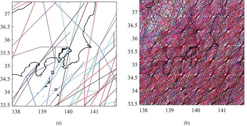
This study analyzes long-term ensemble projections of storm surge for historical and future climate conditions over a 5,000 years period, which gives enough number of events even for particular location. Figure 1 is TC tracks by single ensemble and 100 ensembles of 60 years simulation, showing the benefit of large ensemble for increasing the sample of TC.

Figure 1. TC tracks around Tokyo Bay (200 km × 200 km scale) by (a) single ensemble and (b) 1,000 ensemble simulation.

2.2. Storm surge modeling

Future changes in storm surges were projected using two different empirical models due to large temporal length and computational domain size. First, the storm surge for a regional area was estimated by an empirical formula as a function of the square of the sea surface wind speed, U₁₀, and sea level pressure, P, at particular locations. The empirical model was tuned by a series of numerical simulations based on the nonlinear shallow water equations (NSWE; Kim, Yasuda, and Mase 2008) for 100 major TCs from the stochastic TC model (Nakajo et al. 2014) at the target location. The numerical simulation using the NSWE was conducted using three nested domain starting from a horizontal resolution of Δx = 7.3 km to Δx = 0.81 km, from a high-resolution topography with δx = 10 m provided by the Geospatial Information Authority of Japan. The empirical storm surge model was calibrated based on following equation,

(1) $\eta =a\mathrm{\Delta }P+b{U}_{10}^2$(1)

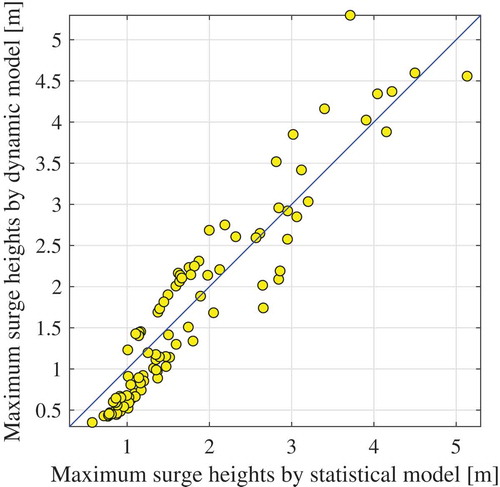
where a is the pressure-induced surge coefficient and b is the wind-induced surge coefficient (b includes bay shape and water depth implicitly). The model coefficient a was fixed as 1 [cm/hPa] and b was tuned for two major bays: Tokyo Bay and Osaka Bay in Japan. The effect of spatial variability of the coastline is implicitly included in the tuned coefficient b. The values of b are 0.00057 and 0.0011 for Tokyo Bay and Osaka Bay, respectively. Figure 2 shows an example of the calibrated model using Equation (1) for Osaka Bay. Although the statistical model has a non-negligible error, with a root mean square error of 0.59 and 0.41 m for Tokyo Bay and Osaka Bay (respectively), they are the first long-term projections of over O(1,000) years by a statistical model at the two target locations for the two bays. Dynamic storm surge modeling for the whole dataset is going to simulate in the near future. Storm surges induced by all TCs passing the target location within 1,000 km were calculated by Equation (1).

Figure 2. Validation of statistical model for maximum surge heights: Osaka Bay.

Second, the future change in storm surge for the global scale was simply estimated same as Equation (1) but the value of b is determined using water depth as,

(2) $b=b_{ref}\cdot h_{ref}/h$(2)

where h is water depth averaged by 50 km radius, $b_{ref}\mathrm{a}\mathrm{n}\mathrm{d}{h}_{ref}$ are 0.0011 and 25 m based on the value at the Osaka bay described above. The upper limit of b is set 0.0022. The spatial resolution of the global statistical storm surge model is the same as the AGCM (Δx = 60 km) and the water depth h for the global model is given by the General Bathymetric Chart of the Oceans (Weatherall et al. 2015). Global storm surges were calculated by the annual maximum wind speed and its SLP based on Equations (1) and (2). Since the global statistical model is not calibrated, the absolute value of storm surge height on a global scale is not discussed; however, the spatial pattern of storm surge height and the rate of change in the surge based on differences between historical and future runs are described. As the value b depends on shape of coastline and bathymetry, the rate of change in the surge is not sensible to the value b in the Equation (2) because of including ratio of characteristic local water depth to reference depth. However, the error can be significant if coast line becomes very complex.

2.3. Contribution analysis of TC intensity and frequency changes to storm surge changes

Contributions of TC intensity and frequency changes to future changes in R-year return value of storm surge are discussed (Shimura, Mori, and Mase 2015). The future change in R-year return value of storm surge ($\mathrm{\Delta }{\eta }_R$) is represented as,

$\mathrm{\Delta }{\eta }_R={\eta }_R^f-{\eta }_R^p$

where ${\eta }_R^f$ and ${\eta }_R^p$ are R-year return value in future and present climate. The variable ${\eta }_R$ is represented by an inverse non-exceedance probability function F and mean yearly occurrence

of storm surge λ and then $\mathrm{\Delta }{\eta }_R$ can be written as follow.

$\mathrm{\Delta }{\eta }_R=F^f\left(\frac{1}{R{\lambda }^f}\right)-F^p\left(\frac{1}{R{\lambda }^p}\right)$

$=F^f\left(\frac{1}{R{\lambda }^p\left(1+\mathrm{\Delta }\lambda \right)}\right)-F^p\left(\frac{1}{R{\lambda }^p}\right)$

where ${\lambda }^f={\lambda }^p\left(1+\mathrm{\Delta }\lambda \right)$. Rewritten by the Taylor series expansion,

$=\left\{F^f\left(\frac{1}{R{\lambda }^p}\right)-F^p\left(\frac{1}{R{\lambda }^p}\right)\right\}-{\dot{F}}^f\left(\frac{1}{R{\lambda }^p}\right)\cdot \frac{1}{R{\lambda }^p}\cdot \frac{\mathrm{\Delta }\lambda }{1+\mathrm{\Delta }\lambda }+E_1$

where $E_1$ includes higher-order terms of the Taylor series expansion. ${\dot{F}}^f$ is replaced by ${\dot{F}}^p+\delta \dot{F}$ and then,

$=\left\{F^f\left(\frac{1}{R{\lambda }^p}\right)-F^p\left(\frac{1}{R{\lambda }^p}\right)\right\}-{\dot{F}}^p\left(\frac{1}{R{\lambda }^p}\right)\cdot \frac{1}{R{\lambda }^p}\cdot \frac{\mathrm{\Delta }\lambda }{1+\mathrm{\Delta }\lambda }-\delta \dot{F}\left(\frac{1}{R{\lambda }^p}\right)\cdot \frac{1}{R{\lambda }^p}\cdot \frac{\mathrm{\Delta }\lambda }{1+\mathrm{\Delta }\lambda }+E_1$

Finally, $\mathrm{\Delta }{\eta }_R$is represented as

(3) $\mathrm{\Delta }{\eta }_R=\left\{F^f\left(\frac{1}{R{\lambda }^p}\right)-F^p\left(\frac{1}{R{\lambda }^p}\right)\right\}-{\dot{F}}^p\left(\frac{1}{R{\lambda }^p}\right)\cdot \frac{1}{R{\lambda }^p}\cdot \frac{\mathrm{\Delta }\lambda }{1+\mathrm{\Delta }\lambda }+\left(E_1+E_2\right)$(3)

where

$E_2=-\delta \dot{F}\left(\frac{1}{R{\lambda }^p}\right)\cdot \frac{1}{R{\lambda }^p}\cdot \frac{\mathrm{\Delta }\lambda }{1+\mathrm{\Delta }\lambda }$

The first term of Equation (3) is represented by the difference in F with the probability of present climate (1/$R{\lambda }^p$), and this term can be considered as a factor of TC intensity change. The second term is represented by F of present climate and frequency change $\mathrm{\Delta }\lambda$, and this term can be considered a factor of TC frequency change. The third term is a residual factor, including frequency–intensity change interaction. In this study, the empirical non-exceedance probability function smoothed by the Kernel smoothing was used for F.

2.4. Representation of tropical cyclones intensities and tracks

Before we discuss future changes in storm surge, it is important to understand that the projected atmospheric climate changes mainly affect TCs briefly. Major regions prone to TCs, including Southeast Asia, East Asia, and eastern US, TCs are generally the key driver of storm surge. Future changes in extreme TCs will be discussed in the next section in more detail. The detection and tracking of TCs for d4PDF use pressure, wind speed, vorticity, and other factors based on the method by Murakami et al. (2012). It basically extract TC center by central pressure and maximum wind speed around TC eye and keep tracking until disappear. The detection threshold value is tuned to adjust to the annual TC number and cyclogenesis number between the observed and historical runs. Although a detailed analysis using the same dataset has been conducted by Yoshida et al. (2017), we will analyze important characteristics of TCs from AGCM for storm surge. Additionally, changes in extra-tropical storms are another important issue for middle to high latitude regions but any analysis of this is excluded here.

Future changes in cyclogenesis number, intensity, and track are compared with satellite observations (Knapp et al. 2010; denoted here as IBTrACS). Data from WMO in IBTrACS was used for comparisons. The cyclogenesis numbers are compared with the projections and IBTrACS directly. The AGCM setup used here includes a 60-km horizontal resolution, which poorly describes the eye wall and vertical convection of a TC when compared with other higher resolution models generally used (e.g. Mori and Takemi 2016). Therefore, validation of TC intensity and assessment of its future change is important to know. The statistical properties of minimum central pressure of TC and annual cyclogenesis number are compared over the globe and WNP directly. The centroids of cyclogenesis, the most developed locations, and cyclolysis locations for characteristic track changes are calculated using the tracks. These three statistical characteristics of TC are important for an impact assessment of storm surge. Although the relation of future changes of TC characteristics and environmental conditions are important, it is still unclear and need to further research in depth. The analysis of TC characteristics itself will not be conducted in this study. Details of the analysis of future change and validation of TC characteristics by d4PDF will be discussed in the next section.

3. Results and discussion

3.1. Future change in tropical cyclone characteristics

We will focus on the analysis of TC characteristics related to storm surge here. The annual cyclogenesis number, probability of minimum central pressure of intense TCs, and changes of tracks are important for impact assessment on storm surges. Validation of basic TC characteristics, spatial distributions over the globe, time series of cyclogenesis number, and frequency of each category 4 and 5 of d4PDF in the historical climate condition have already discussed in Yoshida et al. (2017). Yoshida et al. (2017) showed that the observed TC genesis frequencies for 1979–2010 mostly agree with historical climate conditions (Figure 3 in Yoshida et al. 2017). They also showed that very intense (category 4 and 5) TC occurrences will increase in the WNP but will significantly decrease in d4PDF (Figure 2 in Yoshida et al. 2017).

Based on analysis results from the previous study, we are going to analyze the important TC characteristics for storm surge. First, the intensities of modeled TCs for historical and future climate condition are compared with a dataset of satellite observations (IBTrACS, 2010). Since it is also important to understand the probability of extreme TCs, the non-exceedance probability of the minimum central pressure P_min for each TC is shown in Figure 3 for the historical climate run, the +4K future climate run, and the observed IBTrACS data for global and WNP. Note that the numerical results are based on the whole ensemble product (6,000 years or 5,400 years), but the observed data is based on a period of 36 years (1981–2016). The TC intensities of the historical climate run show good agreement with the observed data in the WNP but are underestimated globally. GCM has bias and need to be corrected generally. Figure 3 shows MRI-AGCM underestimates P_min in the global scale but it gives quite reasonable results in the WNP.

Figure 3. Non-exceedance probability of minimum central pressure P_min for (a) global and (b) WNP (blue line: historical climate, red line: future climate (+4K), black line: observation by IBTrACS, shade: 95% confidence interval).

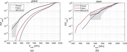
Therefore, the model gives reasonable results for the climatological characteristic of TC intensity in the WNP at least, although the modeled TCs are slightly weaker than TCs in the observed data. The future TC intensity P_min increases dramatically under the +4°C scenario in the WNP but less increased in the global. The deviation of future TC intensity becomes 10 times more frequent for stronger TCs (P_min<920 hPa) in the WNP, if the cyclogenesis number is the same. Note that the signal of future change is also significant in the NAT, which will be shown later.

The future changes in averaged intensity (or power dissipation) of TCs and increasing TC intensity in the WNP are consistent qualitatively with previous studies (e.g. Emanuel 2013). Emanuel (2013) showed +8–80% of power dissipation of TCs globally, with the most evident changes in the North Pacific; Knutson et al. (2010) also demonstrated that the intense TCs will increase on the order of 20% based on GCM ensemble runs. The analysis here indicates that the increase of intense TCs will change monotonically with the minimum central pressure of TCs.

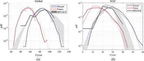
The future cyclogenesis number is expected to decrease due to more stable atmospheric conditions in a warmer climate (e.g. Knutson et al. 2010; Yokoi, Takayabu, and Murakami 2013). A significant decrease in cyclogenesis number is projected globally and in the WNP, as shown in Figure 4. The cyclogenesis number in the future +4K climate run becomes 54.7 #/year (standard deviation σ = 10.5 #/year) for the global average, which is less than the 84.6 #/year (standard deviation σ = 11.5 #/year) for the historical climate run. Additionally, the cyclogenesis number in the WNP in the historical and +4K future climate runs are 28.9 #/year and 14.7 #/year on average, and their standard deviations are 7.8 #/year and 8.0 #/year, respectively. Future cyclogenesis numbers are 35% and 49% less globally and in the WNP, which are larger than values from a RCP8.5 scenario run using the same AGCM (15.2% by Murakami et al. 2012) and GCM ensemble results (6–34% by Knutson et al. 2010). The RCP8.5 scenario reaches a maximum at the end of the 21st century, but the future climate run in this study remains constant from the start to end of this ensemble run. On the other hand, RCP scenario runs by CMIP5 and SRES scenario runs by CMIP3 are transient from present to future. Therefore, the future signal change of mean and deviation in the cyclogenesis number is stronger than the results given by RCP or SRES scenario runs. The range of variation in the ensemble is also large (20–90#/year) and smoothly distributed when compared with a smaller number of ensemble runs. The mega ensemble gives more than double the range in values in the annual cyclogenesis number when compared with a single member (60 years). The range of natural variability of the cyclogenesis number (standard deviation σ = 114 #/year) is 3.8 times larger than the future change (−29.9 #/year). As Knutson et al. (2010) demonstrated, the uncertainty in projection of TC frequency becomes larger depending on the basins and models. The present results show statistically stable projections changing TC frequencies for both globally and the WNP. The use of a mega ensemble, d4PDF, can take account of change in frequency, including natural variability, which is important for assessing natural hazards and impacts on a regional level.

Figure 4. Probability density function of annual cyclogenesis number over (a) global and in (b) WNP (blue solid line: historical climate with 100 ensemble runs, blue dashed line: historical climate with 1 ensemble run, red solid line: future climate (+4K) with 90 ensemble runs, red dashed line: future climate (+4K) with 1 ensemble run, black line: observed (IBTrACS), shade: 95% confidence interval).

Finally, we discuss how TC tracks change due to global warming. TC tracks are expected to shift slightly eastward in the WNP (e.g. Wu and Wang 2004; Yokoi and Takayabu 2009). The TC track shift can occur from a change in the subtropical jet and from intensification of westerly steering flows in the WNP (Yokoi, Takayabu, and Murakami 2013). The shift in TC tracks is important for regional assessments, although the expected change is in the range of a few degrees. For example, if the location where TCs frequently generate shifts to a new location and the total cyclogenesis number decreases globally, the number of TCs approaching the specific target area will increase. Studies investigating changes in TC frequency and intensity have been conducted during the last decade, but investigating how TC tracks shift is not well discussed due to statistically insufficient TC data for the GCMs of each basin. The simple analysis here is to understand changes in characteristics TC tracks by analyzing location shifts of cyclogenesis and others.

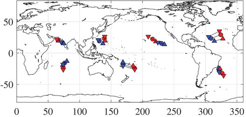
Figure 5 shows the future change in the cyclogenesis location, the most developed location, and the cyclolysis location from d4PDF, respectively. The definition of cyclogenesis and cyclolysis follows Murakami et al. (2012). The locations were calculated by geometric centroids, and in the figure the future change is magnified by a factor of 3 to increase visibility. The mean shifts of cyclogenesis locations from the historical to future climate runs are (Δlon, Δlat) = (1.20°, 1.45°) in the WNP and (4.48°, 1.22°) in the NAT, where a positive value means a shift eastward and northward. The translational shift becomes clearer for cyclolysis. The cyclolysis location shifts from the historical to future climate runs are (Δlon, Δlat) = (3.47°, 1.77°) in the WNP and (5.73°, 3.01°) in the NAT (unit degrees), and therefore the change is significant at higher latitudes (or during the latter part of a TC’s lifetime). The order of track shift in the longitudinal direction is 2–3 times greater than that in the latitudinal direction, and the shift increases from genesis to disappearance. Following our previous study for the CMIP3/CMIP5 data analysis with SRES A1B and RCP8.5 (Mori 2012), the mean shifts in cyclolysis locations are (Δlon, Δlat) = (2.86°, 0.74°) in the WNP and (3.58°, 1.63°) in the NAT. The results of the historical run are basically consistent with previous studies.

Figure 5. Future changes of centroids of TCs (upward triangle: cyclogenesis, circle: most developed, downward triangle: cyclolysis, blue: historical climate, red: future climate (+4K)). Changes are magnified by factor of 3.

Three future changes in TC characteristics, track, intensity and frequency, will strongly influence future changes in storm surge heights. Next, we will discuss how future storm surge will change depending on the change in TC characteristics under the +4K warmer climate condition.

3.2. Future changes in storm surge height

3.2.1. Projection for Tokyo and Osaka Bay

Future projections of storm surge height were conducted using two different methods that depend on target region and accuracy, as described in Section 2. First, we will discuss regional storm surge assessment using a calibrated, local storm surge model at two important mega coastal cities, Osaka Bay and Tokyo Bay in Japan. As the occurrence of severe storm surge is extremely low, the return period of storm surge height is generally discussed for engineering design and assessment.

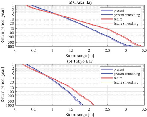
Figure 6 shows the extreme value distribution of regional projections of storm surge heights in Osaka Bay and Tokyo Bay in Japan, respectively. The top two historical, highest storm surges in Osaka Bay were occurred with TC Nancy in 1961 and TC Jebi in 2018, which yielded a 2.85 m water surface elevation (including a 0.41 m astronomical tide; the storm surge height was 2.45 m) and caused 192 causalities and a 3.29 m water surface elevation (including a 0.51 m astronomical tide; the storm surge height was 2.78 m) and caused 13 causalities, respectively. The minimum central pressures of TC Nancy was 888 hPa and became 930 hPa at landfall. The minimum central pressures of TC Jebi was 915 hPa and became 950 hPa at landfall. Since 1961, there have been no other severe storm surge events until TC Jebi in 2018 in Osaka Bay. Therefore, it is difficult to estimate return periods of extreme storm surge in Osaka Bay. Moreover, there is no modern historical record of over 2 m in Tokyo Bay; although several severe storm surges did occur in the 19th century. Other locations face a similar problem with long-term assessments, given the infrequent occurrence of extreme weather phenomena yielding large storm surges. Figure 6(a) for Osaka Bay indicates that the historically highest surge height of 2.4 m corresponds to a 141-year return period in the historical run and corresponds to a 45-year return period in the future climate run (or 3.1 times more frequent in the future). The future climate condition shows shorter intervals between extreme surge events, which is similar to results for a case study for NY (Lin et al. 2012), although they used a statistical TC model instead of GCMs. Similar figure changes in storm surge can be observed in Tokyo Bay as shown in Figure 6(b).

Figure 6. Future change in extreme distribution of storm surge height in Osaka Bay and Tokyo Bay, Japan. (Blue line: historical climate, red libne: future climate (+4K), thick colored line: empirical non-exceedance probability function, thin colored line: smoothed function).

The d4PDF can estimate extreme storm surge events without extrapolation by using extreme value analysis directly. The storm surge heights in the future climate condition with short return periods are slightly smaller than those in the historical climate, but the heights become larger with longer return periods. These storm surge height characteristics in the future climate are balanced between decreasing cyclogenesis frequency and stronger TC intensity. We analyzed how changes in characteristics contribute to storm surges using statistical analysis described in Section 2.3. Figure 7 shows the contribution of the TC characteristics to future change in storm surge: frequency change (red line), intensity change (blue line), and the residual (green line) for two bays. Note that the intensity change includes both change in intensity and TC track shifts and the residual is the frequency–intensity change interaction and higher order error. For the case study of Osaka Bay, the future change in total storm surge changes sign from negative to positive at the 4-year return period, and the future change becomes positive for longer return periods. The total future change in storm surge heights starts at −0.15 m for a 1-year return period and increases up to a maximum of +0.43 m for a 80-year return period. The future change due to TC frequency has a constant negative contribution of about 0.2–0.25 m due to less frequent TC genesis over all of the return periods. Contrarily, intensity change has a positive contribution, monotonically increasing up 0.6 m until a 50 year return period. The residual is small and remains within ±0.05 m. Therefore, change in intensity, including TC track shift, is significant for assessing long-term impacts.

Figure 7. Future change components in extreme distribution of storm surge height in Osaka Bay, Japan. (Thick black line: total change of surge height, red solid line: change due to frequency, blue solid: change due to intensity and track shifts, green line: residual).

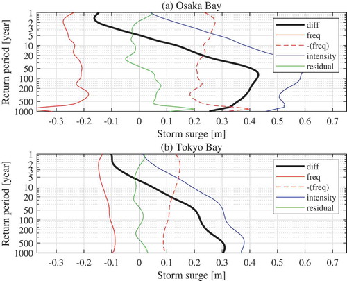
Following the contribution analysis of future changes in storm surge, TC intensity change reaches a maximum around a 50 year return period and becomes constant, although TC frequency change gives a constant, negative effect at about 1/3 of the TC intensity change value. It is difficult to separate the contributions of change due to intensity and track shift, but the influence of track shift is not negligible. A similar change in future storm surge heights can be observed for Tokyo Bay and Ise Bay in Japan (see Tokyo Bay results in Figure 7(b)). Overall, projected future changes in storm surge heights are about 0.5 m, and reach a maximum around the 50- to 100-year return periods for the two bays. This corresponds to about 60% of the projected mean sea-level rise of 0.83 m for the RCP8.5 scenario (IPCC-AR5 WGI 2013), and the two different phenomena occur at the same time.

3.2.2. Global projection

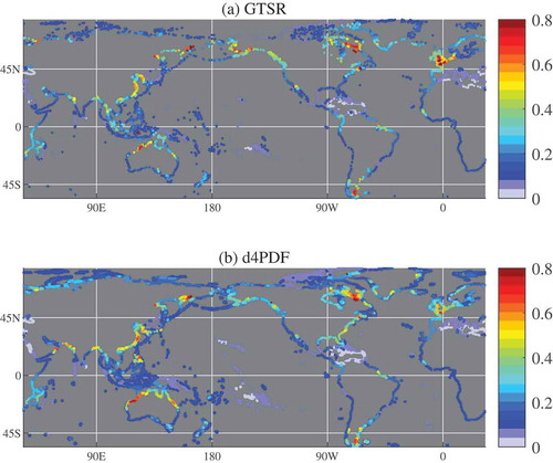
It is important to know future changes in storm surge heights worldwide; however, it is too expensive to simulate storm surge by the method shown in the previous paragraph. Hence, we project the future change ratio of storm surge heights between historical and future runs using a simple statistical model without tuning. First, the comparison of spatial pattern of 100-year return value for storm surge is shown here. Muis, Aerts, et al. (2016) provide the global extreme sea level reanalysis dataset (so-called GTSR) and 100-year return value of extreme sea level is available freely (Muis, Aerts, et al., 2016). Although the extreme sea level consists of tide and storm surge, our analysis just focuses on storm surge. Here, the 100-year return value of extreme sea level was calculated by adding the standard deviation of tide to the 100-year return value of storm surge not considering joint probability between tide and storm surge. The standard deviation of tide was derived from TPXO model (Egbert and Erofeeva 2002). If the maximum value of tide during 1951–2010 is larger than that of extreme sea level, the maximum value of tide is used. Figure 8 shows the qualitative comparison of 100-year return value of extreme sea level between reanalysis data (GTSR: Muis, Verlaan, et al. 2016) and this study. The value in this figure is normalized by being divided by the global maximum value for qualitative comparison. The spatial patterns of current study show good agreement with GTSR data. The results of this study show relatively larger values along the south coast of Japan, the Philippine coast, the Oman coast, and the south and east coast of the US that are prone to intense TC. However, GTSR has underestimation bias of TC (Muis et al. 2017). Therefore, it can be considered that the extreme storm surge at the region prone to TC in this study is plausible.

Figure 8. Comparison of 100-year return value of global extreme sea level along the coast derived from (a) reanalysis data (GTSR; Muis et al., 2016) and (b) this study. The value at each location is normalized by the global maximum value (unit: ratio).

Figure 9 shows the future percent change in storm surge heights and sea surface winds for a 100-year return period. The 100-year return value for storm surge is generally less reliable when a small sample size is used – for example, if historical or 20–50 years of data is used for analysis (e.g. Nakajo et al. 2014). Here we calculated 100-year return values from 6,000 and 5,400 years of data using a nonparametric method without extreme value analysis.

Figure 9. Future percent change in sea surface wind speeds (contour) and storm surges (coast line) in 100-year return periods. The right colorbar shows the range of sea surface wind speed change, the bottom colorbar shows the range of storm surge change, unit: percentage).

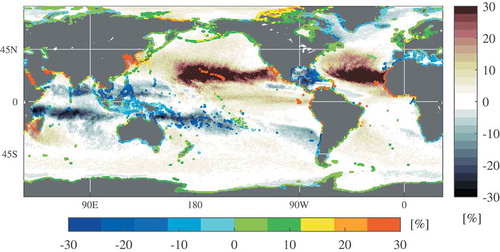
The areas where 100-year wind speeds exceed 40 m/s are located at the middle latitudes or at the Polar Regions and are especially notable in the WNP and the Eastern North Pacific (ENP) due to TC activity. The spatial distribution of 100-year return wind speed values in the historical run is similar to results from the JRA-55 analysis data (figure not shown). Regarding future change in wind speed, it is expected to increase in the Northern Hemisphere and decrease in the Southern Hemisphere by d4PDF. Although trends and intensity differ from satellite observation (e.g. Young, Zieger, and Babanin 2011) and GCMs (e.g. Knutson et al. 2010), here we have extreme changes without extrapolations (or fitting by distributions). Large areas with an increase or decrease of more than 20% relative to the historical climate values are located in the middle latitudes and extend in the longitudinal direction in both hemispheres. The regions with negative, relative values are mainly located in the Southern Hemisphere; they result from a decreasing TC frequency and weaker TC intensity in future climate projections for those areas by same analysis for the South Indian Ocean, the Southern Pacific Ocean and the Southern Atlantic Ocean in the Section 3.1.

A detailed analysis of the wind speed change is necessary and is consistent with a previous study based on the CMIP5 (e.g. Figure 2 in Mendelsohn et al. 2012). Such large, future change in extreme wind speeds is caused by a change in TC track shifts and intensity changes. The projected future change for storm surges also has a similar tendency because of the change in extreme wind speeds. Future 100-year return values of storm surge increase 20% along the East Asian eastern and US western coasts, although future 100-year return values of wind speed increase 10% due to TCs in these areas. A moderate, future change in storm surge within a 10% increase is found in the higher latitudes; this is due to a change in polar circulation in both hemispheres. These changes in the extreme storm surges depend on the length of return periods. Note that as we discussed in the previous section for Tokyo Bay and Osaka Bay, a warmer climate gives lower storm surge heights for shorter return periods (<10 years) but gives larger surge heights for longer return periods. Therefore, the results in Figure 9 show one part of projections and detail of assessment needs depends on the locations. Additionally, while changes in extra-tropical storms were not analyzed in detail here, changes more than 10% in the higher latitude in the WNP, the Northern Atlantic, the North Sea, and the Polar Regions can be seen in Figure 9. Changes in wind speed by the extra-TCs will be stronger in the higher WNP but will not be significant in the higher Northern Atlantic. As such, it is necessary to analyze how extra-TCs and related storm surges will change in the near future.

To summarize the above discussion, extreme changes in storm surge mainly occur due to changes in TC frequency, intensity, and track as illustrated in Figures 6 and 7. Although the projected changes in extreme wind speed and surge depends greatly on the GCM and future scenario used, it is important to assess impacts and start exploring adaptation strategies for coastal hazards by projecting both sea level rise (SLR) and storm surge changes in future climate conditions. Note that a bias correction for wind speed and pressure is necessary in order to obtain quantitative projections, due to the coarse grid size (60 km) used for the TC modeling (Yasuda et al. 2014). Additionally, projected spatial distributions of future change in storm surge differ from spatial distribution of SLR shown in IPCC-AR5. Although the projected SLR is significant in ocean current system, such as Kuroshio but the projected storm surge changes are mainly located middle latitude in the Northern Hemisphere.

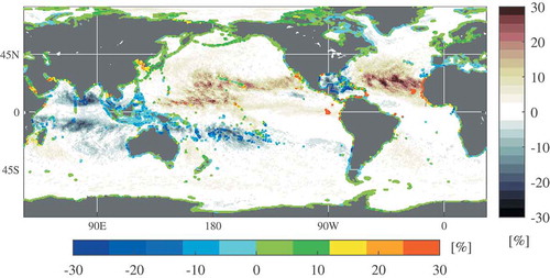
Finally, note that the sensitivity of storm surge as a function of temperature rise is also important to know. The shorter length (2,051–2,110 years × 54 members = 3,240 years) of +2K warming experiment as a subset of d4PDF will be available soon. The preliminary results are shown here. Figure 10 shows the future percent change in storm surge heights and sea surface winds for a 100-year return period. Compared with Figure 9, the projected future change of +2K warming experiment is similar in spatial pattern to that of +4K warming experiment, but the magnitude is smaller by 1/2 roughly than +4K warming experiment. This result can indicate pattern scaling by temperature change to future change in storm surge works well (e.g. Mitchell 2003).

Figure 10. Same as Figure 9 (+4K warming experiment) but for +2K warming experiment.

4. Conclusion

The projection of future storm surge heights worldwide has been discussed based on analysis from mega ensemble experiments, the so-called d4PDF, for an extreme future climate condition using a constant +4°C warmer condition (compared with the pre-industrial period). Based on the mega ensemble results (6,000 years for historical runs and 5,400 years for future climate runs), Future changes in extreme 100-to-1,000-year-rare tropical-cyclone-events and their related storm surges can be projected without using statistical extrapolation.

Characteristics of the projected future changes in extreme storm surges are summarized as follows:

1. TCs will decrease in frequency but increase in intensity, and the mean tracks will shift. Therefore, the future change in TC disaster risks will change depending on the changes in frequency, intensity, and track in the warmer climate for specific locations.

2. Storm surges are expected to increase about 0.3–0.45 m in Tokyo Bay and Osaka Bay in Japan.

3. Storm surges over the globe are expected to increase 10–30% in the middle latitudes around 15–35°N but are expected to decrease in the Southern Hemisphere. Surge changes are related to the future change in TC activities.

4. Storm surges in the future climate are moderately expected to increase in the higher latitudes due to changes in extreme winds in the high latitude regions.

Although quantitative values of global storm surge heights are not shown due to the difficulty of storm surge modeling on a global scale, relative changes in storm surge are discussed qualitatively on a global scale. The future projection of storm surge worldwide is very important and will be investigated in more detail in the near future.

This study used AGCM projections with horizontal 60 km resolution and it is insufficient to resolve TCs in detail (e.g. Emanuel 2013). The use of super resolution GCM with 20 km or finer resolution, downscaling by RCM or bias corrections need to project extreme TCs in detail. Additionally, changes in extra-TCs and related storm surges are important to know in detail. Furthermore, the influence of sea-level rise is an important facet of assessing the impact of climate change in low-lying areas of these regions. Combining future changes in extreme storm surge and sea-level rise is important in order to understand how climate change may influence risk in coastal regions.

Acknowledgments

This study was supported by the Integrated Research Program for Advancing Climate Models (TOUGOU), the Social Implementation Program on Climate Change Adaptation Technology (SI-CAT), the Data Integration and Analysis System (DIAS), which are sponsored by the Ministry of Education, Culture, Sports, Science and Technology of Japan (MEXT). The part of this research was also supported by Environment Research and Technology Development Fund (ERDF). This study utilized the database for Policy Decision making for Future climate change (d4PDF), which was produced using the Earth Simulator as “Strategic Project with Special Support” of JAMSTEC.

Disclosure statement

No potential conflict of interest was reported by the authors.

Additional information

Funding

This work was supported by the Japan Society for the Promotion of Science [Kakenhi]; MEXT [Social Implementation Program on Climate Change Adaptation Technology]; MEXT [Integrated Research Program for Advancing Climate Models]; Environment Research and Technology Development Fund of Japan [2-1712].

References

- Aerts, J. C. J. H., W. J. W. Botzen, K. Emanuel, N. Lin, H. de Moel, and E. O. Michel-Kerjan. 2014. “Evaluating Flood Resilience Strategies for Coastal Megacities.” Science 344 (6183): 473–475. doi:10.1126/science.1248222.
- Bender, M. A., T. R. Knutson, R. E. Tuleya, J. J. Sirutis, G. A. Vecchi, S. T. Garner, and I. M. Held. 2010. “Modeled Impact of Anthropogenic Warming on the Frequency of Intense Atlantic Hurricanes.” Science 327 (5964): 454–458. doi:10.1126/science.1180568.
- Egbert, G. D., and S. Y. Erofeeva. 2002. “Efficient Inverse Modeling of Barotropic Ocean Tides.” Journal of Atmospheric and Oceanic Technology 19 (2): 183–204. doi:10.1175/1520-0426(2002)019<0183:EIMOBO>2.0.CO;2.
- Emanuel, K. A. 2013. “Downscaling CMIP5 Climate Models Shows Increased Tropical Cyclone Activity over the 21st Century.” Proceedings of the National Academy of Sciences 110 (30): 12219–12224. doi:10.1073/pnas.1301293110.
- Hallegatte, S., C. Green, R. J. Nicholls, and J. Corfee-Morlot. 2013. “Future Flood Losses in Major Coastal Cities.” Nature Climate Change 3 (9): 802–806. doi:10.1038/nclimate1979.
- IPCC-AR5 WGI. 2013. The physical science basis. Contribution of Working Group I to the Fifth Assessment Report of the Intergovernmental Panel on Climate Change. 1535.
- Ishii, M., A. Shouji, S. Sugimoto, and T. Matsumoto. 2005. “Objective Analyses of Sea‐Surface Temperature and Marine Meteorological Variables for the 20th Century Using ICOADS and the Kobe Collection.” International Journal of Climatology 25 (7): 865–879. doi:10.1002/(ISSN)1097-0088.
- Kim, S. Y., T. Yasuda, and H. Mase. 2008. “Numerical Analysis of Effects of Tidal Variations on Storm Surges and Waves.” Applied Ocean Research 30 (4): 311–322. doi:10.1016/j.apor.2009.02.003.
- Knapp, K. R., M. C. Kruk, D. H. Levinson, H. J. Diamond, and C. J. Neumann. 2010. “The International Best Track Archive for Climate Stewardship (Ibtracs) Unifying Tropical Cyclone Data.” Bulletin of the American Meteorological Society 91 (3): 363–376. doi:10.1175/2009BAMS2755.1.
- Knutson, T. R., J. L. McBride, J. Chan, K. Emanuel, G. Holland, C. W. Landsea, I. M. Held, J. P. Kossin, A. K. Srivastava, and M. Sugi. 2010. “Tropical Cyclones and Climate Change.” Nature Geoscience 3 (3): 157. doi:10.1038/ngeo779.
- Lin, N., K. A. Emanuel, J. A. Smith and E. Vanmarcke. 2010. “Risk Assessment of Hurricane Storm Surge for New York City.” Journal of Geophysical Research: Atmospheres 115(D18). doi:10.1029/2009JD013630.
- Lin, N., K. Emanuel, M. Oppenheimer, and E. Vanmarcke. 2012. “Physically Based Assessment of Hurricane Surge Threat under Climate Change.” Nature Climate Change 2 (6): 462–467. doi:10.1038/nclimate1389.
- Mendelsohn, R., K. Emanuel, S. Chonabayashi, and L. Bakkensen. 2012. “The Impact of Climate Change on Global Tropical Cyclone Damage.” Nature Climate Change 2 (3): 205–209. doi:10.1038/nclimate1357.
- Mitchell, T. D. 2003. “Pattern Scaling: An Examination of the Accuracy of the Technique for Describing Future Climates.” Climatic Change 60 (3): 217–242. doi:10.1023/A:1026035305597.
- Mizuta, R., H. Yoshimura, H. Murakami, M, Matsueda, H. Endo, T. Ose, K. Kamiguchi et al. 2012. “Climate Simulations Using MRI-AGCM3. 2 With 20-Km Grid”. Journal of the Meteorological Society of Japan. Ser. II 90: 233–258. doi:10.2151/jmsj.2012-A12.
- Mizuta, R., A. Murata, M. Ishii, H. Shiogama, K. Hibino, N. Mori, O. Arakawa, et al. 2017. “Over 5000 Years of Ensemble Future Climate Simulations by 60 Km Global and 20 Km Regional Atmospheric Models.” Bulletin of the American Meteorological Society (BAMS), July: 1383–1398. doi:10.1175/BAMS-D-16-0099.1.
- Mori, N. 2012. Projection of Future Tropical Cyclone Characteristics Based on Statistical Model. Cyclones Formation, Triggers and Control, 24. New York, USA: Nova Science Publishers.
- Mori, N., M. Kato, S. Kim, H. Mase, Y. Shibutani, T. Takemi, K. Tsuboki, and T. Yasuda. 2014. “Local Amplification of Storm Surge by Super Typhoon Haiyan in Leyte Gulf.” Geophysical Research Letters 41 (14): 5106–5113. doi:10.1002/2014GL060689.
- Mori, N., and T. Takemi. 2016. “Impact Assessment of Coastal Hazards Due to Future Changes of Tropical Cyclones in the North Pacific Ocean.” Weather and Climate Extremes 11: 53–69. doi:10.1016/j.wace.2015.09.002.
- Muis, S., M. Verlaan, H. C Winsemius, J. C. Aerts, and P. J. Ward. 2016. “A Global Reanalysis of Storm Surges and Extreme Sea Levels.” Nature Communications 7, 11969.
- Muis, S., J. C. Aerts, M. Verlaan, P. J. Ward, and H. C. Winsemius. 2016. “Global Tide and Surge Reanalysis (GTSR) (2016).” 4TU.Research Data, access April 2018. doi:10.4121/uuid:aa4a6ad5-e92c-468e-841b-de07f7133786
- Muis, S., M. Verlaan, R. J. Nicholls, S. Brown, J. Hinkel, D. Lincke, A. T. Vafeidis, P. Scussolini, H. C. Winsemius, and P. J. Ward. 2017. “A Comparison of Two Global Datasets of Extreme Sea Levels and Resulting Flood Exposure.” Earth’s Future 5: 379–392. doi:10.1002/eft2.2017.5.issue-4.
- Murakami, H., Y. Wang, H. Yoshimura, R. Mizuta, M. Sugi, E. Shindo, Y. Adachi, et al. 2012. “Future Changes in Tropical Cyclone Activity Projected by the New High-Resolution MRI-AGCM.” Journal of Climate 25 (9): 3237–3260. doi:10.1175/JCLI-D-11-00415.1.
- Nakajo, S., N. Mori, T. Yasuda, and H. Mase. 2014. “Global Stochastic Tropical Cyclone Model Based on Principal Component Analysis and Cluster Analysis.” Journal of Applied Meteorology and Climatology 53 (6): 1547–1577. doi:10.1175/JAMC-D-13-08.1.
- Peduzzi, P., B. Chatenoux, H. Dao, A. De Bono, C. Herold, J. Kossin, F. Mouton, and O. Nordbeck. 2012. “Global Trends in Tropical Cyclone Risk.” Nature Climate Change 2 (4): 289. doi:10.1038/nclimate1410.
- Sasaki, H., K. Kurihara, I. Takayabu, and T. Uchiyama. 2008. “Preliminary Experiments of Reproducing the Present Climate Using the Non-Hydrostatic Regional Climate Model.” SOLA 4: 25–28. doi:10.2151/sola.2008-007.
- Schiermeier, Q. 2013. “Did Climate Change Cause Typhoon Haiyan?” Nature 11. doi:10.1038/nature.2013.14139.
- Shimura, T., N. Mori, and H. Mase. 2015. “Future Projections of Extreme Ocean Wave Climates and the Relation to Tropical Cyclones: Ensemble Experiments of MRI-AGCM3. 2H.” Journal of Climate 28 (24): 9838–9856. doi:10.1175/JCLI-D-14-00711.1.
- Taylor, K. E., R. J. Stouffer, and G. A. Meehl. 2012. “An Overview of CMIP5 and the Experiment Design.” Bulletin of the American Meteorological Society 93 (4): 485–498. doi:10.1175/BAMS-D-11-00094.1.
- Weatherall, P., K. M. Marks, M. Jakobsson, T. Schmitt, S. Tani, J. E. Arndt, M. Rovere, D. Chayes, V. Ferrini, and R. Wigley. 2015. “A New Digital Bathymetric Model Of The World's Oceans.” Earth and Space Science 2 (8): 331–345.
- Woodruff, J. D., J. L. Irish, and S. J. Camargo. 2013. “Coastal Flooding by Tropical Cyclones and Sea-Level Rise.” Nature 504 (7478): 44–52. doi:10.1038/nature12855.
- Wu, L., and B. Wang. 2004. “Assessing Impacts of Global Warming on Tropical Cyclone Tracks.” Journal of Climate 17 (8): 1686–1698. doi:10.1175/1520-0442(2004)017<1686:AIOGWO>2.0.CO;2.
- Yasuda, T., S. Nakajo, S. Y. Kim, H. Mase, H. Mori, and K. Horsburgh. 2014. “Evaluation of Future Storm Surge Risk in East Asia Based on State-Of-The-Art Climate Change Projection.” Coastal Engineering 83: 65–71. doi:10.1016/j.coastaleng.2013.10.003.
- Yokoi, S., and Y. N. Takayabu. 2009. “Multi-Model Projection of Global Warming Impact on Tropical Cyclone Genesis Frequency over the Western North Pacific.” Journal of the Meteorological Society of Japan. Ser. II 87 (3): 525–538. doi:10.2151/jmsj.87.525.
- Yokoi, S., Y. N. Takayabu, and H. Murakami. 2013. “Attribution of Projected Future Changes in Tropical Cyclone Passage Frequency over the Western North Pacific.” Journal of Climate 26 (12): 4096–4111. doi:10.1175/JCLI-D-12-00218.1.
- Yoshida, K., M. Sugi, R. Mizuta, H. Murakami, and M. Ishii. 2017. “Future Changes in Tropical Cyclone Activity in High-Resolution Large-Ensemble Simulations.” Geophysical Research Letters 44 (19): 9910–9917. doi:10.1002/2017GL075058.
- Young, I. R., S. Zieger, and A. V. Babanin. 2011. “Global Trends in Wind Speed and Wave Height.” Science 332 (6028): 451–455. doi:10.1126/science.1197219.