Development of an imagery-based monitoring system for nearshore bathymetry by using wave breaking density

ABSTRACT

An imagery-based monitoring system was developed for nearshore topography. The system was based on the wave breaking density observed using a land-based camera and calculated the bathymetry using a depth-controlled breaking wave model. The system was applied to the Fukude-Asaba Coast, Shizuoka Prefecture, where rapid topography change was expected around the outlet of pipeline-based sand bypassing. The validity of the system was verified through comparisons with bathymetry survey data. It is observed that the system can successfully capture the nearshore bathymetry change owing to a typhoon. It is also suggested that the accuracy is sensitive to the incident wave properties and therefore can be improved by introducing selective averaging in which only appropriate imageries were used for the depth estimation depending on the target depth zones.

KEYWORDS:

• Nearshore bathymetry monitoring
• image analysis
• Argus
• wave breaking density
• beach deformation

1. Introduction

Fukude-Asaba Coast is a sandy beach in Shizuoka Prefecture, Japan, located in the east of the Ota River mouth (Figure 1). The primary source of beach sediments is the Tenryu River, located 10 km west of the Fukude-Asaba Coast. The longshore sand transport rate is estimated at 130 × 10³ m³/year in the direction to the east (Uda et al. 2013). The construction of breakwaters of the Fukude Harbor has blocked the longshore sediment transport, causing significant deposition on the west side of the harbor and severe erosion on the Fukude-Asaba Coast located on the east side of the harbor (Figure 2). Although various countermeasures have been introduced, such as dredging the navigation channels and bypassing sand by boats and dump trucks from west to east, coastal erosion is still significant on the downdrift coasts. In 2014, Shizuoka Prefecture decided to introduce a pipeline-based sand bypassing system for the first time in Japan, inspired by the successful practice in Australia (Dyson, Victory, and Connor 2001). The system sucks up marine sand deposited on the west side of the harbor with jet pumps, carries it to the east side through a 2.2-km-long pipeline and discharges it on the Fukude-Asaba Coast with a design rate of 80 × 10³ m³/year. As the operation of the system must be conducted with careful and precise monitoring of nearshore environment, it is desired to monitor the nearshore topography change, which is highly variable in broad time scales from hours to decades, with emphasis on understanding the impact/response of the sand bypassing. It is therefore essential to develop a monitoring system of nearshore topography with high resolutions both in time and space.

Figure 1. Fukude-Asaba Coast located 10 km west of the Tenryu River mouth. Sediments are transported from west to east. Waves and tide data used for the bathymetry estimation are obtained from the Ryuyo Wave Station located at the Tenryu River mouth and the Omaezaki tide gauge.

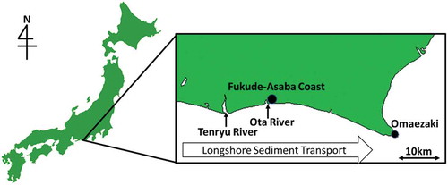
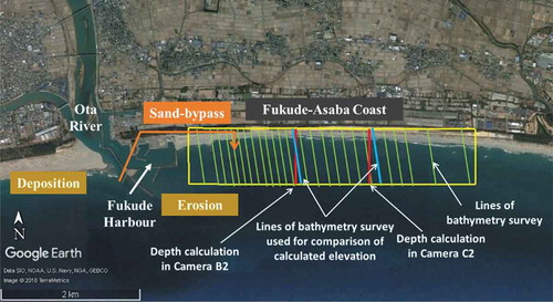
Figure 2. Map of Fukude-Asaba Coast, Shizuoka Prefecture, Japan. Pipeline-based sand bypassing system (indicated by the orange line) carries sediments from west to east with a design rate of 80 × 10³ m³/year.

Coastal Imaging Lab at Oregon State University has developed a coastal monitoring system called Argus Station (Holman and Stanley 2007). It is a nearshore monitoring system based on imagery captured using land-based video cameras, acquiring a large amount of data on nearshore processes, such as tides, waves, currents, and beach morphology with a relatively low cost. Many studies discussed the movement of sand bars and beach morphology cycles by using time exposure (TIMEX) images averaged for 10 to several minutes. Lippmann and Holman (1990) observed that the movement of sand bars was highly variable with short time scales, especially after storms. In addition to qualitative analyses, the imagery-based monitoring system has been used for the quantitative estimation of nearshore bathymetry by inversely using the dispersion relationship based on the wave period and wavelength estimated from the imagery (e.g. Stockdon and Holman 2000). However, the accuracy of the estimation appears to be dependent on the wave conditions and may include significant error owing to the difficulty in measuring wave speed from the movement of wave crests by using land-based cameras situated at limited elevations. The difficulty in the inverse depth estimation using the dispersion relationship was also remarked by Matsuba and Sato (2018) who estimated nearshore bathymetry using an unmanned aerial vehicle. They remarked that the exclusive extraction of swell components with relatively long wave periods is essential to ensure accuracy even in pictures captured from the top.

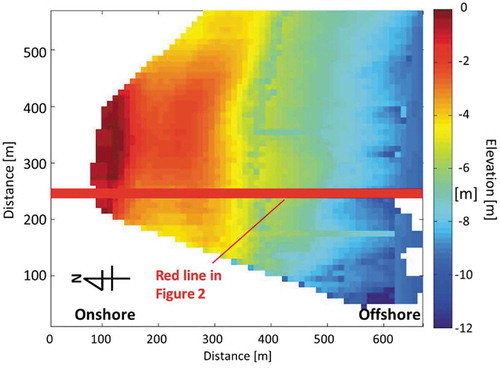
A nearshore bathymetry survey on the Fukude-Asaba Coast is conducted by Shizuoka Prefecture annually with survey lines at the intervals of every 100–200 m illustrated by the green lines in Figure 2. The monitoring frequency and density are designed to evaluate the long-term trend of beach erosion. However, detailed monitoring data with higher frequency and density are required to evaluate the performance of the sand bypassing system although such monitoring will not be allowed by the limited budget and high cost of the bathymetry survey. To complement the scarcity of nearshore bathymetry data, Okabe and Kato (2017) developed a low-cost big-data oriented bathymetry monitoring system by logging the tracks of fishing boats. The color map in Figure 3 illustrates the bathymetry estimated by Okabe and Kato (2017) in which the nearshore bathymetry averaged over 4–6 months was estimated by collecting water depths along the track path of many fishing boats moving around the nearshore area. The system can estimate the nearshore bathymetry with a relatively low cost although the estimation must be restricted to the area with moderate water depth where sufficient number of track paths can be collected by fishing boats tracking school of fish. Figure 3 also shows a typical time-averaged picture (TIMEX) of the eight cameras introduced in this study. Each camera, situated on the top of a pole approximately 20 m above the sea level, captures pictures every 2 s during 10:00–10:21 and 15:00–15:21 every day. The distribution of the whitish area in Figure 3 represents the location of the sand bar variable temporarily and spatially. However, quantitative monitoring of nearshore bathymetry is required to understand the relationship between the beach recovery and the amount of bypassed sand and thus to evaluate the performance of the sand bypassing system. In this study, we considered that the quantitative estimation of depth-controlled wave breaking density through an imagery-based system could be used as a proxy for nearshore bathymetry. Individual snapshots of nearshore imagery are used to estimate the spatial distribution of the wave breaking density, the probability of wave breaking per unit area. The wave breaking density is thereafter used to estimate the bathymetry by introducing an appropriate model for depth-controlled breaking of random waves.

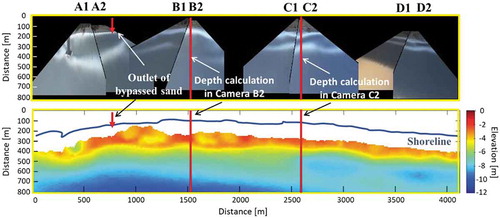
Figure 3. Rectified TIMEX image of eight cameras (top) and the bathymetry estimated by Okabe and Kato (2017) by using fish finder log (bottom). The area is represented by the yellow rectangle in Figure 2. The location of the outlet pipe of sand bypassing is indicated by the arrow. The red lines represent the cross-shore transects analyzed in this study.

2. Monitoring system of nearshore bathymetry by using wave breaking density

Many studies on the transformation of wave heights have been conducted since the 1970s, e.g. Goda (1975), Battjes and Janssen (1978), Thornton and Guza (1983), and Dally, Dean, and Dalrymple (1985), in which various models were presented for the change of nearshore wave heights due to shoaling and breaking. In this study, we assumed that the nearshore wave breaking could be described by Goda’s model for random waves (Goda 1975). The model can calculate the depth-controlled breaking deformation of shoaling random waves with a simple equation by assuming the Rayleigh distribution for incident wave heights. Therefore, for a given bathymetry, the cross-shore distribution of wave breaking density could be estimated using the model. Furthermore, the wave breaking density could also be estimated from a series of snapshots of nearshore imagery. We considered that the video imagery and the wave breaking model could be linked to estimate the bathymetry by using the wave breaking density as a proxy. Goda’s model is a one-dimensional model and does not consider wave breaking in the longshore direction. Therefore, in this study, we considered the wave breaking density as the probability of wave breaking per unit cross-shore distance.

2.1. Estimation of wave breaking density using nearshore imagery

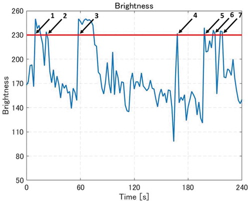
One bathymetry data was estimated for pictures taken in 21 min, therefore 630 pictures were used to make one bathymetry data. The photos captured by the land-based cameras were rectified to the horizontal-plane rectangular coordinates (x,y) based on Holland et al. (1997). The change in RGB brightness of each grid was analyzed. The wave breaking was identified by the rapid increase in the brightness. For a given distance dx in the cross-shore direction, the fraction of wave breaking was calculated by the number of rapid increases divided by the number of total waves. This was then divided by the given distance dx in order to calculate the brightness-based wave breaking density $p_0\left(x,y\right)$, calculated directly from the imagery taken by the land-based cameras using the brightness of pictures, as expressed by Equation (1),

(1) $p_0\left(x,y\right)=\frac{N}{W}\frac{1}{dx},$(1)

where N denotes the number of rapid increases in the brightness exceeding a certain threshold, W is the total number of waves calculated from the mean wave period observed at the Ryuyo Wave Station, located 10 km to the west from the Fukude-Asaba Coast, and dx is the grid size in the cross-shore direction. The threshold of brightness was appropriately determined so as to capture wave breaking accurately. In this study, 230 (maximum 255) was used for the threshold of brightness for all pictures. As an example, the brightness of a certain grid for 240s can be shown as Figure 4. From image analysis, the threshold of brightness was determined at 230, therefore N is 7. If we consider the average wave period to be 6 s and the grid size to be 0.2 m, p₀ is 0.875 (1/m). It is expected that the actual wave breaking density is proportional to $p_0\left(x,y\right)$, which represents the occurrence of wave breaking in a specific horizontal area in the nearshore imagery. However, attention must be paid to the distortion of imagery owing to the conversion of imagery to a rectified image in the horizontal coordinate.

Figure 4. Method to calculate the rapid increase of brightness.

Figure 5 illustrates a schematic diagram of a breaking wave observed from a land-based camera. In the imagery recorded by the camera, each pixel represents a footprint area on the sea surface. The size of the footprint will be larger in the offshore area, where the stretching factor is proportional to $r^2$, where r is the distance from the camera. As the white-colored bright breaking waves tend to be enhanced as compared with dark non-breaking waves, the wave breaking in the area far from the camera tends to be overestimated in proportion to $r^2$. In addition to the stretching in the horizontal plane, the stretching of the steep front face of breaking wave must be considered in the shadow zone of breaking waves. As the shadow stretching factor will be larger when the depression angle $\theta$ of the camera is small, a larger shadow stretching will be introduced for the offshore zone where the depression angle of camera becomes smaller. This will lead to an overestimation of wave breaking in the area far from the camera. Larger breaking wave heights, likely to be observed in the offshore zone, tend to increase the overestimation rate in the area far from the camera. To compensate the overestimation introduced by these mechanisms, we assumed that $p_0$ could be converted to the wave breaking density by multiplying with a decaying function proportional to $r^{-n}$. The empirical coefficient n was determined in this study by the comparisons of $p_0$ and the wave breaking density calculated using Goda’s model along the cross-shore line with known bathymetry. We selected a cross-shore transect, as indicated by the red line in the area of the picture captured using camera B2 in Figures 2 and 3, and assumed the bathymetry profile there as provided by Okabe and Kato (2017). The frequency of breaking waves $p_0$ was calculated along the red line by using the imageries captured with the camera B2. Subsequently, the model-based wave breaking density $p_0^{\prime }$ was calculated using Goda’s model for the given wave properties and bathymetry by Okabe and Kato (2017). The incident wave properties were obtained from those observed at the Ryuyo Wave Station. The ratios $p_0^{\prime }/p_0$ were calculated for five different days and are plotted in Figure 6, where the horizontal axis represents the distance r from the camera. Figure 6 shows that the ratio could be approximated by $r^{-4}$, especially in the offshore area where long-crested wave breaking is observed. It is therefore considered that the corrected wave breaking density p, which is to be used for the estimation of water depth, was calculated from $p_0$ in this study according to the following equation:

(2) $p\left(x\right)=p_0\left(x\right)\times \frac{K}{r^4},$(2)

Figure 5. Shadow zone behind a breaking wave leading to the overestimation of wave breaking density. $\theta$ shows the depression angle, H shows the wave height, r shows the distance between the camera and the wave, $H_c$ shows the height of the camera.

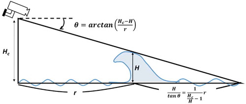
Figure 6. Relationship between the overestimation rate and the distance r from the camera. The overestimation of wave breaking density can be compensated by $r^{-4}$.

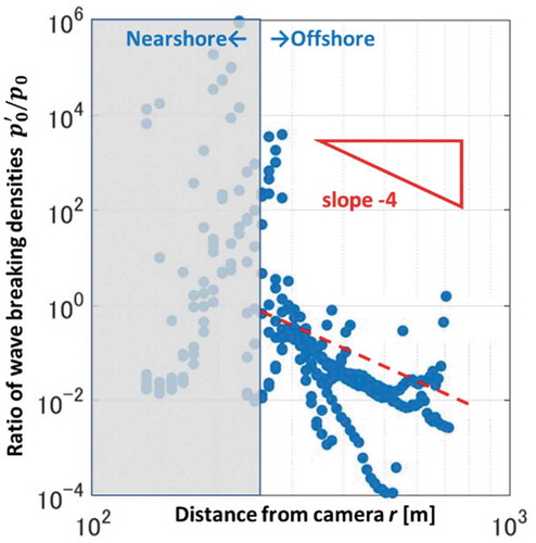
where K [m⁴] is a coefficient to be determined for individual camera conditions. The value of K was determined via a sensitivity test for the relatively less variable offshore bathymetry, by reference to Figure 6, so that the offshore bathymetry can be estimated accurately.

2.2. Estimation of bathymetry based on Goda’s wave breaking model

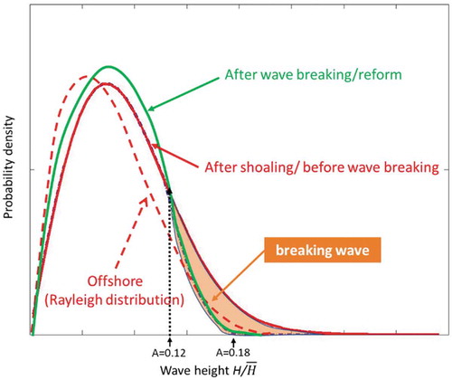
Goda (1975) developed a model to calculate the change of wave height distribution owing to random wave breaking. The model is based on the assumption of the wave breaking density and wave reformation after breaking. In Goda’s wave breaking model, the incident wave height distribution is given as a Rayleigh distribution.

(3) $p_0^{\ast }\left(x^{\ast }\right)=\frac{\pi }{2}{x}^{\ast }exp\left[-\frac{\pi }{4}{x^{\ast }}^2\right],$(3)

where x* is a non-dimensional variable showing the ratio of the wave height and the mean wave height. The change of wave heights at the onshore location will be calculated by considering shoaling and breaking. The wave breaking condition is given by the following equation:

(4) $H_b=A\cdot L_0\left\{1-exp\left[-\frac{1.5\pi h_b}{L_0}\left(1+k\mathrm{t}\mathrm{a}{\mathrm{n}}^s\theta \right)\right]\right\},$(4)

where $H_b$ is the breaking wave height, $L_0$ is the offshore wavelength, h_b is the wave breaking water depth, $\mathrm{t}\mathrm{a}\mathrm{n}\theta$ is the bed slope and $k=15$, $s=\frac{4}{3}$ is a parameter, determined in Goda (1975), to account for the sensitivity of wave breaking on the bed slope. The parameter A represents the probability of wave breaking. Goda (1975) proposed $A=0.12$ for the lower limit and $A=0.18$ for the upper limit. No waves will break if the corresponding A values are smaller than 0.12 whereas all waves will break when the corresponding A values are larger than 0.18. Waves in the range 0.12 < A < 0.18 were assumed to break with probability increasing linearly with A value.

Figure 7 shows a schematic diagram of the wave height distribution at offshore and two nearby locations assumed in the nearshore area. The dashed line represents the Rayleigh distribution in the offshore whereas the red line is the wave height distribution at a nearshore location x and the green line is that at the adjacent onshore location x + dx after shoaling/breaking/reformation in [x, x + dx]. In this diagram, the orange area represents the fraction of waves broken in [x, x + dx], therefore wave breaking density can be calculated by dividing the area of the orange part by dx. Goda’s model assumes that broken waves are reformed in proportion to the probability density of unbroken waves. By repeating this procedure step by step from offshore to onshore, we can estimate the wave breaking density together with wave deformation owing to depth-controlled shoaling and breaking.

Figure 7. Change of wave height distribution before and after wave breaking. H shows the wave height and $\bar{H}$ shows the mean wave height.

The detailed calculation method of the model is as follows. Goda’s model uses Shuto’s shoaling model (1974) to estimate the wave height after shoaling. The wave height distribution after shoaling is $p_1^{\ast }\left(x\right)$. $x_1^{\ast }$ and $x_2^{\ast }$ are the upper and lower limits of the ratio of wave height and mean wave height. $p_r^{\ast }\left(x^{\ast }\right)$ represents the wave height distribution in the Goda’s model before introducing wave reformation.

(5) $x_1^{\ast }=\frac{H_b|A=0.18}{\bar{H}},$(5)

(6) $\begin{array}{c}{x}_2^{\ast }=\frac{H_b|A=0.12}{\bar{H}},\end{array}$(6)

(7) $\begin{array}{c}{p}_r^{\ast }\left(x^{\ast }\right)=p_1^{\ast }\left(x^{\ast }\right):x^{\ast }\le x_2^{\ast }\\ =p_1^{\ast }\left(x^{\ast }\right)-\frac{x^{\ast }-x_2^{\ast }}{x_1^{\ast }-x_2^{\ast }}{p}_1^{\ast }\left(x_1^{\ast }\right):x_2^{\ast }<x^{\ast }\le x_1^{\ast }\\ =0:x_1^{\ast }<x^{\ast }\end{array},$(7)

The probability of the remaining waves is shown by $\alpha$ expressed by Equation (8), therefore the wave height distribution after the reformation of broken waves is shown as $p^{\ast }\left(x^{\ast }\right)$.

(8) $\alpha =\underset{0}{\overset{x_1^{\ast }}{\int }}{p}_r^{\ast }\left(x^{\ast }\right)d{x}^{\ast },$(8)

(9) $p^{\ast }\left(x^{\ast }\right)=\frac{1}{\alpha }{p}_r^{\ast }\left(x^{\ast }\right),$(9)

From the equations above, the wave breaking density can be calculated as $\frac{1-\alpha }{\mathrm{d}\mathrm{x}}$.

In this study, we utilized Goda’s model to calculate the water depth inversely from the wave breaking density estimated using Equation (2) through image analysis. First, by using the significant wave height and the mean wave period given in the offshore, the water depth at the first wave breaking was calculated where the wave breaking density became non-negligible. In this study, the wave breaking density was assumed to be non-negligible if it is larger than 10⁻⁶ (1/m), considering the statistical error in the camera image analysis. Subsequently, the water depth at one-step onshore location was estimated from the wave breaking density such that the calculated wave breaking density from imageries is consistent with the wave breaking density from Goda’s model assuming the most appropriate water depth for the onshore location. This procedure was repeated until the shoreline with the grid size of dx = 10 m.

To confirm the applicability of the inverse depth estimation, we conducted a sensitivity test as shown in Figure 8. A bar-type coastal profile was assumed as shown by the dashed line. The green line represents the wave breaking density calculated using Goda’s model for a specific wave condition with H_1/3 = 2.0 m and $\bar{T}$ = 8.0 s. During the wave shoaling, as indicated in the top panel of Figure 8, wave breaking is developed from larger waves, causing a shift in the wave height distribution to the waves with smaller heights. The wave breaking density becomes large on the bar and becomes smaller behind the bar. Subsequently, by masking the bathymetry, the water depth was inversely estimated by using Goda’s model from the breaking wave density step by step from the offshore to the onshore. The result is shown by the pink line in Figure 8. It is observed that the pink line generally overlaps with the dashed line, thus showing the applicability of the inverse depth estimation. However, it is also noted that the inverse estimation is not applicable where the wave breaking density becomes negligibly small. In this example, the estimation is applicable only in the zone shallower than 5 m where the first wave breaking is observed. The estimation is not applicable, however, in the area behind the sand bar, where no waves will break owing to the large water depth there. In such a situation, as shown by the pink line in Figure 8, the water depth was assumed as the minimum water depth that guarantees no wave breaking.

Figure 8. Change of wave height distribution and wave breaking density for an assumed topography.

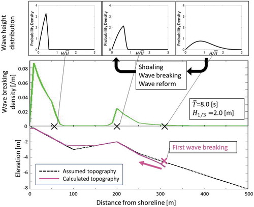
Figure 9 shows the sensitivity tests for different wave conditions. It is observed that the applicable range of the inverse depth estimation is dependent on the incident wave height and period. Larger waves with longer periods tend to expand the applicable zone in the offshore zone whereas the applicability in the shallow zone (behind bar) is better enhanced for smaller waves. In practice, as waves are highly variable daily and hourly, the inverse depth estimation was conducted at various timings under different wave conditions. The final bathymetry was thereafter calculated as an ensemble average of water depth estimations. It is noted that the small discrepancy observed at the first wave breaking as noted in the middle panel of Figure 9 is considered to be due to the ignorance of small breaking events in the area further offshore.

3. Results

The results obtained from the imagery-based inverse depth estimation were compared with annual bathymetry surveys and the bathymetry data compiled from fish finder log by Okabe and Kato (2017). Okabe’s data used for comparison is the average bathymetry for September 2016 to January 2017. The bathymetry was estimated in Tokyo Peil (T.P.), the standard datum in Japan, by accounting for the tide variation by using the tide data at Omaezaki, located 30 km to the east of the Fukude-Asaba Coast (Figure 1).

3.1. Estimation procedures

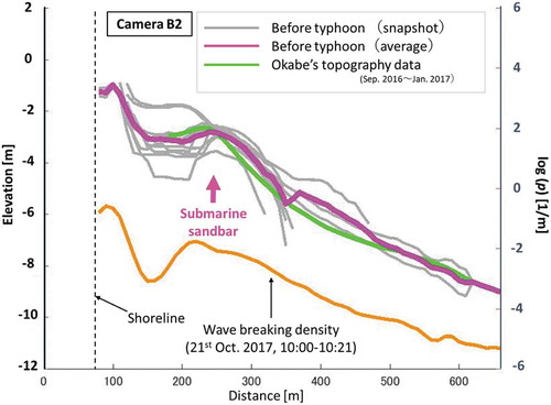
The nearshore bathymetry was estimated by using imageries captured using two cameras, B2 and C2 (Figure 3). Bathymetries in the period from October 2017 to January 2018 were targeted, as significant bathymetry changes were introduced by Typhoon No. 21, which landed at the nearby coast on October 23 2017 with the largest significant wave height of 8.6 m. Figure 10 shows the variation of H_1/3 and the mean wave period in the period from October 11 to October 31, 2017. Clear pictures capturing the depth-controlled wave breakings of moderate long-period waves were selected for 7 days (indicated by pink arrows) before the typhoon impact and 4 days (indicated by blue arrows) after the typhoon. Figure 11 shows an example of rectified imageries of Camera B2 and Figure 12 shows the bathymetry estimated as an ensemble average in the area covered by Camera B2.

Figure 10. Wave conditions in October 2017 and the dates used to calculate water depth.

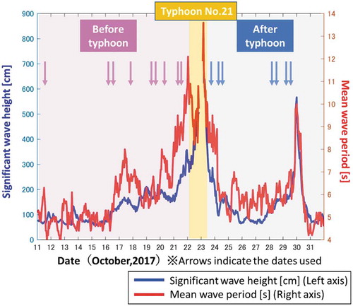
Figure 11. Rectified image of B2 Camera with the line used for the profile comparison.

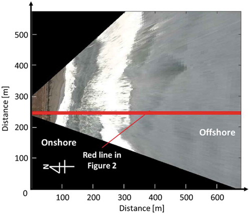
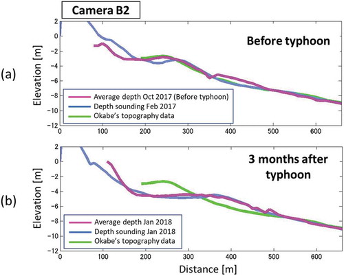
Figure 12. Estimated bathymetry before the typhoon (Camera B2).

3.2. Results of bathymetry survey

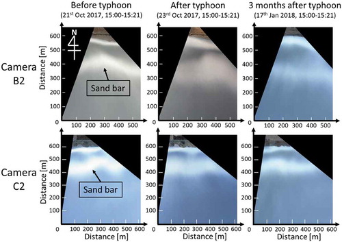
Bathymetry survey using a single-beam sonar is conducted every year by the Shizuoka Prefecture. Data from February 2017 and January 2018 were used to validate the model in this study. Figure 13 shows the result of bathymetry survey along the blue lines in Figure 2. The results were shown along a line perpendicular to the shoreline. It is observed that Okabe’s estimation (green) is consistent with the bathymetry survey in February 2017 (pink). The profiles after the typhoon (orange) indicate significant erosion in the area close to the shore and the accretion in the offshore probably owing to the offshore sand transport developed by the typhoon storm. The longshore sand bar was eroded and moved offshore in the area of Camera B2 whereas the location of the sand bar was less variable in the area of Camera C2 where the erosion close to the shore deepened the trough behind the sand bar. These responses of nearshore topography to the typhoon impact can be qualitatively observed also in the TIMEX image illustrated in Figure 14. The whitish area representing the position of the longshore sand bar became obscured and moved offshore on October 23 2017 and on January 17 2018 for Camera B2 whereas it was less variable for Camera C2. It is also observed that the whitish area for Camera C2 became more significant in January 2018 probably owing to the deepened trough behind the bar.

Figure 13. Nearshore profiles in the area covered by Camera B2 and C2. The bathymetry surveys were conducted in February 2017 and January 2018. Okabe’s data represent the bathymetry in the period from September 2016 to January 2017.

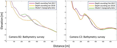
Figure 14. Time-averaged imageries for Camera B2 and C2.

3.3. Results of imagery-based bathymetry estimation in the area covered by Camera B2

Figure 15 shows the wave breaking density and the bathymetry estimated using Camera B2. A typical distribution of the wave breaking density, observed on October 21 2017 at 10:00–10:21, is shown as the orange line by logarithmic scale (right axis). It shows a secondary peak at approximately 120 m from the shoreline, probably representing the location of the longshore sand bar. The gray lines show the bathymetry estimated for nine timings before the typhoon and the dark purple line shows the ensemble average. The green line indicates the bathymetry estimated by Okabe and Kato (2017). The consistency between the dark purple line and the green line demonstrates the validity of the inverse depth estimation developed in this study. Especially, it is noted that the sand bar located 120 m offshore from the shoreline is successfully reproduced.

Figure 15. Coastal profile with wave breaking density for the area of Camera B2 before the typhoon in October 2017.

Figure 16 shows the bathymetry estimated after the typhoon in October 2017. The comparisons before and after the typhoon, as illustrated in Figure 17, indicate that the sand bar moved approximately 50 m offshore after the typhoon, probably owing to offshore-ward sand transport by erosional storm waves. Figure 18 shows the comparison of profiles with the bathymetry surveys, demonstrating the applicability of the model.

Figure 16. Coastal profile with wave breaking density for the area of Camera B2 after the typhoon in October 2017.

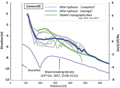
Figure 17. Comparison of bathymetries and wave breaking density before and after Typhoon No. 21.

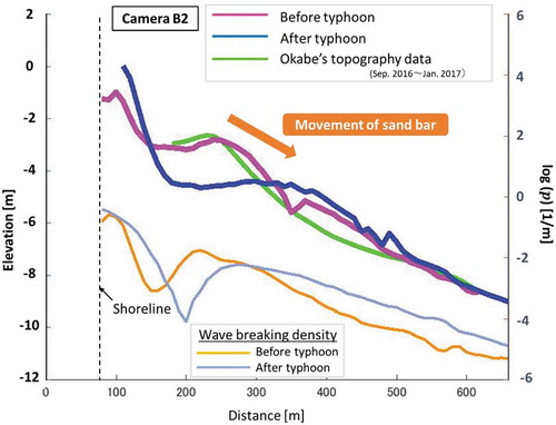
Figure 18. Comparison of profiles with depth sounding data in the area of Camera B2.

3.4. Results of imagery-based bathymetry estimation in the area covered by Camera C2

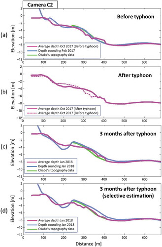
Figure 19 shows the comparisons of nearshore profiles in the area covered by Camera C2. An ensemble average was obtained for 11 snapshots selected from pictures captured in January 2018. Notably, the movement of the sand bar for Camera C2 was less significant than that for Camera B2, which is consistent with the bathymetry survey data shown in Figure 13. The imagery-based estimations successfully represent the erosion close to the shore and the slight accretion in the offshore zone. However, as illustrated in Figure 19(c), the model fails to estimate the deepening of the trough of the sand bar observed three months after the typhoon. This is considered to be due to the difficulty of the inverse depth estimation in the area where only a small number of waves will break, as confirmed in Figure 9. To overcome the difficulty, a selective averaging technique is introduced such that the average is obtained only for snapshots expected with moderate accuracy. As confirmed from a comparison of Figure 9(a,c), the estimation obtained using smaller waves achieves better accuracy in the trough zone as more waves will break in the trough zone as compared with the poor estimation obtained using larger waves breaking mostly in the offshore zone. It is therefore considered that the selective ensemble average obtained only using smaller waves will better estimate the deepened trough behind the sand bar. Figure 19(d) shows the estimation based on such selective averaging, in which only six snapshots with smaller waves were used out of the total 11 snapshots used in the estimation in Figure 19(c). The better representation of deepened trough in Figure 19(d) suggests the advantage of the selective averaging in which only qualified snapshots with moderate accuracy are selectively used depending on the target zones.

Figure 9. Topography calculation under different wave conditions ($\bar{T}$ is the mean wave period and $H_{1/3}$ is the significant wave height).

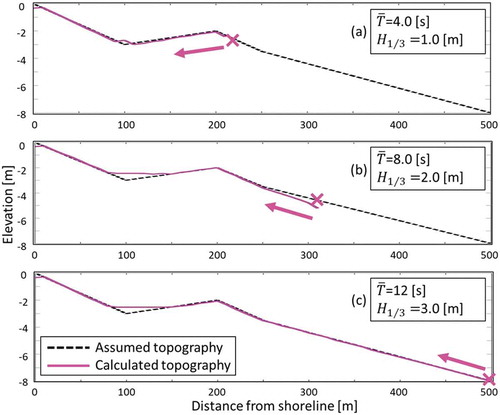
Figure 19. Bathymetry estimation using Camera C2. (a) Before typhoon (b) after the typhoon (c) 3 months after typhoon (d) 3 months after typhoon with selective averaging.

4. Concluding remarks

An imagery-based monitoring system was developed for nearshore topography. The spatial distribution of wave breaking density was estimated from snapshot imageries of the nearshore wave field captured using land-based cameras with appropriate image corrections. The nearshore bathymetry was estimated by comparing the wave breaking density calculated using the depth-controlled breaking wave model proposed by Goda (1975). The system was applied to the Fukude-Asaba Coast, Shizuoka Prefecture, where rapid topography change was expected owing to the continuous operation of pipeline-based sand bypassing. It is observed that the system can successfully estimate the nearshore bathymetry changes owing to a typhoon occasionally attacking during the monitoring period, such as the erosion close to the shore, accretion in the offshore, and movement of the longshore sand bar to the offshore. It is also suggested that the accuracy of the bathymetry estimation will be enhanced by introducing a selective averaging procedure in which only appropriate imageries with moderate wave heights were used for the depth estimation depending on the target depth zones.

Further studies are required on the robustness of the system for various incident wave properties and on the selection criteria to exclude the estimation with poor accuracy.

Acknowledgments

This study was financially supported by JSPS KAKENHI Grant Number JP17K18898. The authors appreciate the Shizuoka Prefecture and Dr. Okabe, Toyohashi University of Technology, for providing the bathymetry data.

Disclosure statement

No potential conflict of interest was reported by the authors.

Additional information

Funding

This work was supported by the The Japan Science of Promotion of Science [17K18898].

References

- Battjes, J. A., and J. P. F. M. Janssen. 1978. “Energy Loss and Set-Up Due to Breaking of Random Waves.” Proceedings of 16th Coastal Engineering Conference, Vol. 1, 569–587.
- Dally, W. R., R. G. Dean, and R. A. Dalrymple. 1985. “Wave Height Variation across Beaches of Arbitrary Profile.” Journal of Geophysical Research 90 (C6): 11917–11927. doi:10.1029/JC090iC06p11917.
- Dyson, A., S. Victory, and T. Connor. 2001. “Sand Bypassing the Tweed River Entrance: An Overview.” Coasts & Ports 2001: Proceedings of the 15th Australasian Coastal and Ocean Engineering Conference, the 8th Australasian Port and Harbour Conference: 310–315.
- Goda, Y. 1975. “Deformation of Irregular Waves Due to Depth-Controlled Wave Breaking.” Report of the Port and Harbour Research Institute 14 (3): 59–106.
- Holland, K., R. A. Holman, T. C. Lippmann, J. Stanley, and N. Plant. 1997. “Practical Use of Video Imagery in Nearshore Oceanographic Field Studies.” IEEE Journal of Oceanic Engineering 22 (1): 81–92. doi:10.1109/48.557542.
- Holman, R. A., and J. Stanley. 2007. “The History and Technical Capabilities of Argus.” Coastal Engineering 54 (I6–I7): 477–491. doi:10.1016/j.coastaleng.2007.01.003.
- Lippmann, T. C., and R. A. Holman. 1990. “The Spatial and Temporal Variability of Sand Bar Morphology.” Journal of Geophysical Research 95 (C7): 11575–11590. doi:10.1029/JC095iC07p11575.
- Matsuba, Y., and S. Sato. 2018. “Nearshore Bathymetry Estimation Using UAV.” Coastal Engineering Journal 60 (I1): 51–59. doi:10.1080/21664250.2018.1436239.
- Okabe, T., and S. Kato. 2017. “Monitoring Bathymetric Changes in Fukude Fishing Port and Adjacent Coast.” Journal JSCE, B2 (Coastal Engineering) in Japanese 73 (2): I_607-I_612. doi: 10.2208/kaigan.73.I_607.
- Shuto, N. 1974. “Nonlinear Long Waves in a Channel of Variable Section.” Coastal Engineering in Japan, JSCE 17: 1–12. doi:10.1080/05785634.1974.11924178.
- Stockdon, H. F., and R. A. Holman. 2000. “Estimation of Wave Phase Speed and Nearshore Bathymetry from Video Imagery.” Journal of Geophysical Research 105 (C9): 22015–22033. doi:10.1029/1999JC000124.
- Thornton, E. B., and R. T. Guza. 1983. “Transformation of Wave Height Distribution.” Journal of Geophysical Research 88 (C10): 5925–5938. doi:10.1029/JC088iC10p05925.
- Uda, T., T. San-Nami, T. Ishikawa, Y. Ito, N. Shiraishi, and J. Sato. 2013. “Effect of Ground Subsidence to Beach Changes on Omaezaki Coast.” Journal of JSCE, B2 (Coastal Engineering) 69 (2): I_666–670.