Quantifying blue carbon for the largest salt marsh in southern British Columbia: implications for regional coastal management

Abstract

Understanding blue carbon storage and accumulation prior to engineering projects is essential for assessing the potential co-benefit of carbon storage for natural climate solutions. This study collected sediment cores from the western portion of Boundary Bay, Delta, British Columbia (BC), where implementation of a living dike pilot project is planned to alleviate impacts of sea level rise. Total carbon stocks were 10,034 ± 3,148 Mg C for the western 140 ha of marsh, with stocks averaging 83.3 ± 29.3 Mg C/ha (high marsh) and 39.3 ± 24.2 Mg C/ha (low marsh). Carbon accumulation rates (CARs) exhibited substantial variability, ranging from 19.5 to 454 g C/m²/yr (median 70.1 g C/m²/yr). Both stocks and accumulation rates were at least 45% lower than globally averaged estimates, likely due to the shallow depth and dominant vegetation type of the marsh. Despite historical modifications to the marsh, our study indicates that the western marsh has expanded by about 20% since 1930, which we estimate increased carbon stocks by about 1,549-1,698 Mg C. This study’s quantification of carbon stocks and CARs is an important first step towards leveraging the co-benefit of salt marshes for improved management, restoration, and preservation. However, additional data are needed to document the greenhouse gas budgets for carbon accounting purposes, along with exploration of law and policy issues related to carbon stewardship in a multi-jurisdictional coastal environment. We outline subsequent research needed for salt marshes such as Boundary Bay to be included in voluntary carbon markets in British Columbia.

KEYWORDS:

• Blue carbon
• salt marsh
• carbon accumulation
• British Columbia
• coastal management

Introduction

Salt marshes are intertidal ecosystems found on sheltered marine coastlines that can sequester large amounts of “blue carbon” in their soils, relative to their small areal extent (Chmura et al. 2003; Bridgham et al. 2006; Drake et al. 2015). Their effective carbon sequestering abilities are primarily due their high primary productivity, ongoing sediment deposition, ongoing burial of autochthonous vegetation (litter and roots), and relatively low decomposition rates (Callaway et al. 2012; Drake et al. 2015). Due to the vertical sediment accretion in response to rising sea level, carbon stocks and accumulation rates may increase over time (Stagg et al. 2016). Furthermore, polyhaline (salinity >18) tidal marshes have been shown to have negligible methane emissions (Poffenbarger, Needelman, and Megonigal 2011). Seawater contains sulfate ions which undergo sulfate reduction and outcompete methanogenesis in soil, thus limiting methane production (Kroeger et al. 2017). As a result, polyhaline marshes can become net carbon sinks that can help mitigate climate change.

Salt marsh ecosystems are highly influenced by the tide and can be separated into two distinct high and low marsh zones (Pennings and Callaway 1992; Weinmann et al. 1984). The low marsh is inundated daily by the tide whereas the high marsh is only flooded once or twice a month during high tides and storms (Pennings and Callaway 1992; Weinmann et al. 1984). Elevation differences of only a few centimeters are sufficient to alter the intertidal environment from a low marsh to a high marsh zone (Scholten and Rozema 1990; Zedler et al. 1999). Still, these zones have markedly different vegetation, such that the low marsh is dominated by species that are more tolerant to waterlogged soils and higher salinities (Pennings and Callaway 1992; Weinmann et al. 1984). Moreover, these zones can have different carbon stock and accumulation abilities (Connor, Chmura, and Beth Beecher 2001; Chmura et al. 2003; Elsey-Quirk et al. 2011; Pendleton et al. 2012; Duarte et al. 2013; Ouyang and Lee 2014). Therefore, the proportion of high and low marsh zones is important for estimating carbon storage capacity, especially when designing and managing an ecologically engineered marsh such as a living dike system.

In addition to their importance as carbon sinks, coastal wetlands can help coastal communities with climate change adaptation through shoreline stabilization and storm surge and flood protection (Lau 2013). Unfortunately, coastal ecosystems are threatened yearly by reclamation, development, and sea level rise, with estimates ranging from 1% to 2% losses annually (Bridgeham et al, 2006; Duarte et al. 2008). As a result, coastal communities are increasingly vulnerable to flooding associated with sea level rise and storm intensification (Spalding et al. 2014). Increasingly, communities are exploring strategies to harness ecosystem services in coastal wetlands through conservation, restoration, and management (Sutton-Grier, Wowk, and Bamford 2015).

Recent calls for nature-based solutions suggest that enhanced engineering of coastal wetlands could provide sustainable approaches to protect communities against effects of sea-level rise while serving as potential carbon sinks (Temmerman et al. 2013). These approaches, while promising, require further investigation to understand the extent of their benefits and limitations (Möller 2019; Seddon et al. 2020). Information about the underlying sedimentary dynamics and carbon sequestration processes are needed about individual projects to assess their long-term effectiveness as protective barriers and carbon sinks. The paucity of salt marsh carbon storage and sequestration data in specific regions creates difficulties in designing regional plans that incorporate a role for blue carbon, either as a co-benefit for other ecosystem services or an explicit target for carbon markets or policies (Pendleton et al. 2012, 2013; Ullman, Bilbao-Bastida, and Grimsditch 2013; Sutton-Grier and Moore 2016; Sheehan et al. 2019; Villa and Bernal 2018). In regions with little or no data, using generalized global estimates rather than site-specific data could result in inaccurate estimates of carbon burial rates and stocks (Ewers Lewis et al. 2018). This is because local carbon dynamics can vary in response to many site-specific factors, including vegetation assemblages, hydrodynamic pressures, sediment type, age, and geological processes (Zhou et al. 2006; Mahaney, Smemo, and Gross 2008; Elsey-Quirk et al. 2011; Connor, Chmura, and Beecher 2001; Ouyang and Lee 2014; Kelleway et al. 2017). The Pacific coast of Canada is notably absent from recent synthesis efforts because of the lack of published data (Chmura et al. 2003; Ouyang and Lee 2014). Thus, quantifying carbon stocks and carbon accumulation rates can help to inform national, regional, and local carbon strategies as well as conservation and rehabilitation efforts (Sutton-Grier and Moore 2016; Sheehan et al. 2019; Moomaw et al. 2018).

Boundary Bay, British Columbia (BC) is the largest salt marsh in southwestern Canada, playing a pivotal role for critical habitat, flood protection, and as a potentially important blue carbon ecosystem. The marsh is within an area designated as a provincial Wildlife Management Area since 1986 (Government of British Columbia 2020 a). More recently, the government of Canada has committed to help fund a “living dike” pilot project with the City of Delta, City of Surrey, and the Semiahmoo First Nation, in which small sections of the Boundary Bay marsh will be managed and enhanced (City of Surrey n.d.; Readshaw, Wilson, and Robinson 2018). Over the course of the 9-year project, an adaptive management framework will be used to design, implement, monitor, and evaluate the effectiveness of different methods, materials, and approaches. A living dike system that integrates protection and enhancement of salt marsh ecosystems with management of existing conventional dikes can provide coastal flood protection for communities landward of the dikes, by buffering wave energy and mitigating storm surge. This hybrid approach – combining management and protection of coastal ecosystems with traditional, engineered flood protection – may be more cost-effective and use less raw materials than conventional approaches alone (Van Der Nat et al. 2016). The living dike in Boundary Bay is also intended to support the adaptation of the salt marsh to sea level rise and avoid its loss through coastal squeeze (Readshaw, Wilson, and Robinson 2018).

In addition to protecting vulnerable agricultural land, residential areas, and regional infrastructure, management and protection of the salt marsh in Boundary Bay could help mitigate climate change by maintaining and increasing the salt marsh carbon storage capabilities (Sutton-Grier and Moore 2016). Incorporating carbon as a measured co-benefit of nature-based shoreline protection requires estimation of the marsh’s long-term carbon storage potential and would be relevant to design considerations of larger-scale implementation of the living dike in Boundary Bay. At the policy level, the regional government of Metro Vancouver has recently included Boundary Bay and its existing salt marsh in a regional carbon storage data set that is aimed at supporting connections between land-use decision-making and carbon storage in the region (Wellham and Seely 2019).

Quantification of blue carbon ecosystem services in places such as Boundary Bay Marsh also presents new opportunities to meet carbon reduction goals via the emerging economic carbon market, in Canada and other countries (Ullman, Bilbao-Bastida, and Grimsditch 2013; Sheehan et al. 2019). British Columbia has legislated greenhouse gas reduction targets of 40% below 2007 by 2030, 60% by 2040, and 80% by 2050 (Climate Change 2007), and since 2008 has had a carbon tax that applies to the purchase and use of fossil fuels (Government of British Columbia n.d.). Salt marshes are currently not part of any regulatory offset program in British Columbia nor any regulated carbon market. However, coastal wetland restoration activities are currently available through the voluntary carbon market (Sheehan et al. 2019), which allows government authorities, corporations, associations, and individuals to offset GHG emissions outside of legally mandated GHG reduction commitments. Several protocols and certification standards have been developed to support integrity in the voluntary carbon market (Vanderklift et al. 2019). These all emphasize a high standard in establishing a baseline for carbon accounting projects as well as robust and transparent monitoring (IPCC 2000; Emmer et al. 2015; American Carbon Registry 2017).

This research provides new and essential baseline data regarding the role of salt marshes in carbon storage and sequestration on the north Pacific coast of North America and the Lower Mainland of British Columbia. Our study provides important quantification of the ongoing sequestration of blue carbon in the western portion of the salt marsh in Boundary Bay, Delta, British Columbia, prior to its modification from the development of a living dike project. We also introduce a new volumetric approach to measure carbon stocks, which may prove useful for accurate estimation of total carbon stocks in young, shallow marshes. This case study demonstrates the kind of information that is crucial for integrating the blue carbon dynamics of a salt marsh ecosystem into regional coastal planning of nature-based solutions for climate change mitigation.

1. Methods

1.1. Study Area

Our study focuses on the largest part of the salt marsh situated in the western side of Boundary Bay, Delta, B.C (Figure 1). The western portion of the marsh is 8.0 km long and 0.5 km wide at its widest point, with a total area of 1.4 km² (140 ha). Sampling occurred in the far western ~0.55 km² (55 ha) portion of the marsh. The salt marsh is bounded to the north by a large, man-made dike. While the original date of construction is unknown, the dike was strengthened and heightened in 1948 (Shepperd 1981). The land north of the dike consists of farmland, a small airport (Boundary Bay Airport), a golf course, and sparse residential housing.

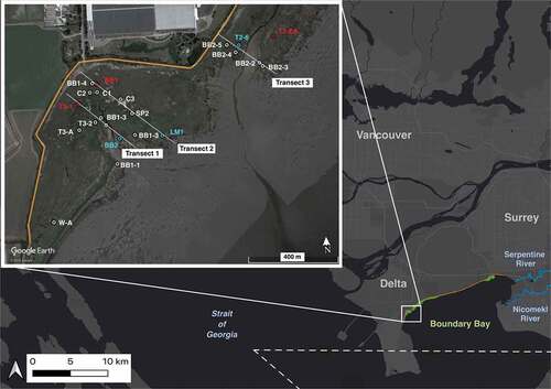
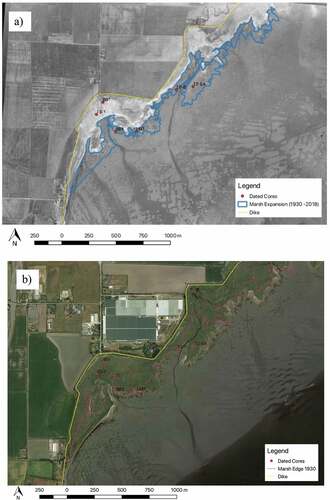
Figure 1. Map of the location of Boundary Bay marsh, Delta, B.C. in relation to the Lower Mainland, B.C. the inlay map shows the location of three transects and coring sites in the western portion of Boundary Bay. All cores were collected for carbon analysis. The red dots indicate the three high marsh cores that were dated, the blue dots indicate the three low marsh cores that were dated, and white dots indicate all other cores. The orange lines in the base map and the inlay represent the dike. In the base map, the green shading represents the marsh, and the white dashed line represents the Canada–United States Border

The water near the leading edge of the marsh has a salinity of 24 to 29, similar to that of the Strait of Georgia (Swinbanks and Murray 1981). The Serpentine and Nicomekl rivers flow into Mud Bay in Surrey, B.C., approximately 7 km east of the study area (Baldwin and Lovvorn 1994). The tides in Boundary Bay are a mixed semidiurnal type, with two high and two low tides (Shepperd 1981). The mean tidal range is 2.7 m, with a maximum spring tidal range of at least 4.1 m and a minimum neap tidal range of 1.5 m (Swinbanks and Murray 1981).

Boundary Bay is considered the inactive southern flank of the Fraser Delta because most sediment from the Fraser River plume is blocked from entering the bay by Point Roberts peninsula (Swinbanks and Murray 1981). Sediment is brought into the bay via loose sediment from the cliffs at Point Roberts. The Serpentine and Nicomekl rivers discharge only a minor amount of sediment into the eastern part of the bay (Swinbanks and Murray 1981).

1.2. Field sampling

All sampling occurred at the widest portion of the western marsh, west of 72nd St, in Delta, BC (Figure 1). Sampling included vegetation surveys, sediment coring, and marsh depth measurements.

For sediment coring, three transects were chosen to characterize variability across the transition from high to low marsh (Table A1). Transects were parallel to one another positioned perpendicular to the dike’s edge. We attempted to evenly sample from both high and low marsh zones. Additional sites away from transect lines were sampled to capture full variability in marsh vegetation (Figure 1).

Low and high marsh zones were differentiated through vegetation surveys at each coring site. At each site, a 50 × 50 cm quadrat was placed, and percent cover of each species was recorded. Sampling sites were then classified as high or low marsh based on the dominant plant species (Table A2). The only exception to this marsh zonation were two cores sampled in salt pannes (cores SP2 and C1). Salt pannes are depressed, poorly drained areas where tidal water pools and salinity concentrate through evaporation (Pennings and Bertness 2001). Salt panne sampling sites were distinguishable in the high marsh through visible depressions in the marsh, standing water in the middle of the depression or desiccated bare soil, and Salicornia virginica monocultures that clearly transitioned to high marsh plant species at the edges of the panne. These sites were considered high marsh cores because they do not experience the same tidal pressures as the low marsh and are only filled with tidal waters during storms or high tides (Pennings and Bertness 2001).

Twenty-two sediment cores were collected using a Livingstone piston corer. Eight cores were collected in the summer of 2014, two cores in June 2017, and 12 cores during May–September 2018. Each sediment core was extruded from the corer onto PVC tubing that was cut in half. The 5.5-cm diameter cores were stored in the Parks Canada laboratory and refrigerated at 4°C. One “core” (Core W-A) was a pit that was dug until sand was reached, and samples were taken every 5 cm.

During coring, the piston corer was pushed into the ground to the depth of refusal (Table A1). Depth of refusal is considered a reasonable estimate of organic soil thickness because it assumes that organic soil is easier to penetrate than underlying sands and/or bedrock (Howard et al. 2014). For this study, we assumed that the underlying sand layer was formed prior to marsh initiation (Howard et al. 2014). Once cores were extracted from the corer, the length of the core was measured along with the depth of the core hole from which they were extracted (length of core penetration, or depth of refusal). Core lengths were generally shorter than the depth of refusal due to compression that was caused by the core extraction method (Table A1).

For estimates of volume, carbon stocks, and carbon accumulation rates (below), a compression factor was needed to correct for sediment compaction during the coring process. Compression was estimated by dividing the length of core penetration by the length of core recovered:

(1) $CompressionFactor=\frac{lengthofcorepenetration\left(cm\right)}{lengthofcore\left(cm\right)}$(1)

This correction factor was used to estimate the corrected depth (Howard et al. 2014):

(2) $CorrectedDepth=compressionfactor\times depthofsamplefromcore\left(cm\right)$(2)

The compression factor is used for the entire length of the core, which assumes that all sections of the core are compacted equally. We recognize that this assumption may be an oversimplification as compaction is may vary with the core due to several factors (Howard et al. 2014; Morton and White 1997). We also note that depth of core penetration was not recorded (and therefore compression not assessed) for cores collected in summer 2014 (high marsh n = 3 and low marsh n = 5) and in two cores collected in summer 2018 (high marsh n = 2). These 10 cores were not used to calculate any metrics that required uncompressed data (e.g. volume carbon stocks and CARs).

Depth profiles, vegetation surveys, and GPS coordinates were recorded at an additional 154 sampling sites throughout the western portion of the marsh (Table A3, Figure A6). Depth profiles were collected by pushing a metal meterstick down until the sand layer was felt; this depth is considered the depth of organic matter. Depth profiles were used to calculate marsh thickness to provide a more robust estimate of marsh carbon stock. Vegetation surveys were used to create an accurate map of low marsh and high marsh zones (Tables A2, A3; Figure 4, A5).

1.3. Marsh area and volume

To estimate the area of high and low marsh zones, QGIS 3.0 tools were used with a 50 × 50 m resolution Google satellite base map compiled from images taken on July 23, 2018. High and low marsh zones were delineated by eye using differences in vegetation color on Google Satellite base map imagery (Figure 4 and Figure A5). The halophyte-dominated low-marsh plant assemblage was a lighter shade of green compared to the darker green of the high marsh plant assemblages (Chastain 2017). Additionally, high and low marsh zones were identified using vegetation surveys at 176 sample points (22 sediment core sites and 154 additional sample sites). The designations determined using vegetation surveys aligned perfectly with the visual delineations made using satellite color (Table A2 and Table A3). As a result, the remaining 55% (77 ha) of high and low marsh area to the east of the sampled zone was delineated only by eye using 2018 Google Satellite base map vegetation coloration (Figure 4).

Air photos taken on May 5, 1930, (provided by NRCan, National Earth Observation Data) allowed us to estimate changes in the areal extent of the western marsh between 1930 and 2018. Using QGIS 3.0 tools, the 1930 air photo was georeferenced and then overlaid on the 50 × 50 m Google Satellite base map to measure how much the marsh had grown (Figure 5).

To test some new, volumetric approaches for measuring carbon stocks, we also estimated the volume of a specified bounded area in the western portion of Boundary Bay west of 72nd street using ArcMap 10.3 tools. The marsh volume was calculated using 139 depth profiles and a kriging geostatistical method (Figure A6). A second, simpler volumetric method involved multiplying the bounded area by the average of the 22 un-compacted core lengths.

1.4. Laboratory analyses

Sediment cores (n = 22) were split in the laboratory and measurements of dry bulk density, percent carbon, soil carbon density, and carbon stock made for every core (Table 1). Sedimentology was logged for cores that were sampled in summer 2017 and 2018 (n = 14) (Figure A1). One-cm³ volumes of sediment were sampled at 1-cm increments for the entire length of each core. Samples were oven-dried (72 hrs at 60 °C) and weighed to determine dry bulk density (DBD, g/cm³). Samples were then ground using a mortar and pestle, combusted in a muffle furnace (4 hrs at 550 °C), and weighed to calculate loss-on ignition (LOI), to quantify the fraction of organic carbon lost (Howard et al. 2014):

(3) $\mathrm{\%}LOI=\left(\frac{D{W}_i-D{W}_f}{D{W}_i}\right)\times 100$(3)

Table 1. Summary of core sediment data (depth of core, dry bulk density (DBD), average percent carbon (%C), average soil carbon density (SCD), and carbon stock) collected for cores in Boundary Bay, Delta, B.C. The % of total core C stock represents the percentage of the total core carbon found above the 13 cm horizon.^a

Core ID	Depth of core (cm)	Average DBD (g/cm^3) ± SD	Average %C ± SD	Average SCD (gC/cm^3) ± SD	Carbon stock (MgC/ha)	Carbon Stock at 13cm	% of total core C stock
High Marsh Cores
T3 - 2	25	0.32 ± 0.09	21.1 ± 6.1	0.061 ± 0.010	159.2	79.1	49.7
T3 - A	27	0.42 ± 0.09	11.1± 5.4	0.043± 0.011	115.4	66.9	58.0
C2	16	0.76 ± 0.31	6.5 ± 6.6	0.031 ± 0.017	52.7	46.8	88.8
C3	20	0.59 ± 0.23	9.0 ± 7.5	0.047 ± 0.037	78.0	54.1	69.4
BB1	21	0.51 ± 0.23	10.3 ± 2.4	0.039 ± 0.013	82.4	57.9	70.3
BB1-4	18	0.41 ± 0.12	11.4 ± 3.7	0.044 ± 0.011	79.1	60.9	77.0
BB1-3	24	0.78 ± 0.41	5.3 ± 5.4	0.024 ± 0.019	58.7	47.2	80.4
BB2-5	20	0.56 ± 0.46	12.2 ± 2.5	0.034 ± 0.020	68.9	55.3	80.3
T2-EA	20	0.44 ± 0.26	14.0 ± 7.9	0.045± 0.024	93.7	68.7	73.3
W-A	45	0.41 ± 0.29	20.6 ± 12.2	0.069 ± 0.025	62.5	n/a
C1	21	0.55 ± 0.16	10.0 ± 4.6	0.048 ± 0.010	106.2	63.9	60.2
SP2	15	0.66 ± 0.26	6.5 ± 5.6	0.030 ± 0.020	44.3	44.3	100
T3 - 1	21	0.50 ± 0.21	8.6 ± 5.4	0.034 ± 0.016	81.9	51.7	63.1
Average ± SD	23 ± 7	0.53 ± 0.14	11.3 ± 4.9	0.042 ± 0.013	83.3 ± 29.3	58.1 ± 10.3	72.5 ± 14.0
Low Marsh Cores
BB1 - 2	25	0.61 ± 0.25	3.9 ± 2.8	0.018 ± 0.011	42.6	24.8	58.2
BB2	23	0.94 ± 0.16	1.2 ± 1.1	0.010 ± 0.008	23.5	17.6	74.9
BB1 - 1	17	0.74 ± 0.21	2.3 ± 2.4	0.013 ± 0.012	22.4	20.2	90.2
BB2 - 4	19	0.58 ± 0.21	2.8 ± 2.5	0.013 ± 0.009	22.6	20.8	92.0
BB2 - 3	13	0.42 ± 0.14	6.7 ± 3.6	0.029 ± 0.015	31.7	31.7	100
BB2 - 2	20	0.83 ± 0.33	1.6 ± 1.8	0.008 ± 0.008	12.0	11.8	98.3
T2 −6	27	0.41 ± 0.27	8.6 ± 5.0	0.024 ± 0.012	68.0	41.5	61.0
LM1	29	0.78 ± 0.30	3.9 ± 6.1	0.015 ± 0.016	44.7	35.2	78.7
LM2	29	0.54 ± 0.19	7.2 ± 5.4	0.030 ± 0.010	86.3	47.3	54.8
Average ± SD	22 ± 6	0.65 ± 0.18	4.3 ± 2.6	0.018 ± 0.008	39.3 ± 24.2	27.9 ± 11.8	78.7 ± 17.6

^a13 cm horizon was chosen because it represented the shallowest core and therefore allowed us choose a constant depth horizon that used all cores.

where $D{W}_i$ is the initial dry weight and $D{W}_f$ is the dry weight after burning.

In a subset of samples (cores BB1 (n = 8) and BB2 (n = 8)), organic carbon content (%C) was also determined by measuring the total carbon and inorganic carbon contents in the same samples, using CHN elemental and coulometric analysis, respectively. Elemental analysis (EA) was completed at the University of British Columbia’s Department of Earth, Ocean, and Atmospheric Sciences (Postlethwaite et al. 2018; Chastain 2017; Howard et al. 2014). Replicate analysis of certified reference material (MESS-3 standards) had a standard deviation of ± 0.01% for total carbon content. Percent inorganic carbon (IC) was measured using a UIC CM5014 CO₂ coulometer connected to a UIC CM5130 acidification module at the Climate, Oceans, and Paleo-Environments laboratory at Simon Fraser University. Percent IC was negligible in all samples (maximum = 0.01% IC) and assumed to be zero for all %C calculations (Howard et al. 2014; Postlethwaite et al. 2018; Hodgson and Spooner 2016; Chastain 2017).

A regional relationship between %C and %LOI (Figure A2; Eqn 4)(4) $\mathrm{\%}C=0.44\left(\mathrm{\%}LOI\right)-1.33$(4) was calculated with a least-squares regression, using %C and %LOI data from this study and additional paired data from marshes on the Pacific coast of Canada (Chastain 2017). We combined the data to develop a robust regional relationship between %C-%LOI for west coast marshes. Although Boundary Bay salt marsh is larger and more complex than the Pacific coast marshes, the vegetation communities were similar, we used the same methods to calculate %C and %LOI, and both data sets had negligible amounts of IC. Including data from Chastain (2017) does not markedly change the relationship, which is not surprising given that the relationship between %C and %LOI is relatively homogenous among tidal salt marshes (Howard et al. 2014; Craft, Seneca, and Broome 1991). The fraction of organic carbon (%C) in each sample was then calculated using the following relationship (r² = 0.97):

(4) $\mathrm{\%}C=0.44\left(\mathrm{\%}LOI\right)-1.33$(4)

1.5. Carbon stocks

In estimating carbon we first measured carbon stocks in all cores (n = 22, n = 13 for high marsh, n = 9 for low marsh) and then scaled up these measurements to estimate the amount of carbon per hectare (Mg C/ha) in the high marsh, low marsh, and the entire western portion of Boundary Bay marsh (Figure 4). In all cores, carbon stocks were only calculated for the layers where % carbon was non-negligible, and all carbon stocks are represented as organic carbon stocks. The carbon stock for each core $Cstoc{k}_{core}$ (g C/cm²) was calculated as (Howard et al. 2014):

(5) $Cstoc{k}_{core}\left(\frac{gC}{c{m}^2}\right)=\sum _{i=0}^{n}SC{D}_i\times 1cm$(5)

where n is length of the core (cm) in which % C is greater than zero, and $SC{D}_i$ is the soil carbon density (SCD) measured at 1-cm intervals (i):

(6) $SCD\left(\frac{gC}{c{m}^3}\right)=\left(\frac{\mathrm{\%}C}{100}\right)\times DBD\left(\frac{g}{c{m}^3}\right)$(6)

where %C is the carbon content and DBD is the dry bulk density for each interval.

The marsh carbon stock (Mg C) for the entire western marsh was calculated by adding together the total low marsh and high marsh carbon stocks, which were estimated by multiplying the average carbon stocks for each strata (high and low marsh) by the marsh strata areas determined in QGIS3.0 tools (Table 1; Figure 4).

To understand potential uncertainties in total carbon stock estimates, we calculated carbon stocks (Mg C) using three different methods for a specified bounded area of the marsh where we were able to complete detailed depth profiles (Table 2; Figure A6): (1) a traditional approach, (2) a kriging volumetric approach, and (3) a simplified volumetric approach. The first, traditional approach is most widely used; carbon stock is estimated by multiplying the area of the marsh by the average of carbon stocks calculated from the sediment cores. The traditional method involved multiplying the average C stock (combining high and low marsh data) by specified bounded area. For the traditional approach, SCDs do not need to be uncompressed because carbon stock is calculated by summing the total amount of carbon in each core down to marsh initiation (Eqn 5(5) $Cstoc{k}_{core}\left(\frac{gC}{c{m}^2}\right)=\sum _{i=0}^{n}SC{D}_i\times 1cm$(5) ), which ensures that the total amount of carbon is included in the carbon stock determination. The second and third volumetric methods are new approaches using the volume of the marsh multiplied by the average sediment carbon density estimated from the sediment cores. The kriging volumetric approach used the kriging geostatistical method to derive marsh volume from 136 depth profiles. This volume was then multiplied by the average of the uncompressed SCD ($\frac{gC}{m^3}$) for all cores:

(7) $UncompressedSCD=AverageSCD\times CompressionFactor$(7)

Table 2. Comparison of carbon stock estimates (Mg C) for a specified bounded area in the western portion of Boundary Bay, derived from three different methods: the traditional method using the area (m²) multiplied by the average core carbon stocks, and two volumetric methods that multiply volume (m³) by the average soil carbon density (g C/cm³). Volumes are estimated using a kriging geostatistical method (see text), and a simplified approach of multiplying average core lengths by area (m²). A is the bounded marsh area, $\overline{\mathit{C}\mathit{s}\mathit{t}\mathit{o}\mathit{c}{\mathit{k}}_{\mathit{c}\mathit{o}\mathit{r}\mathit{e}}}$ ^b is the average of the carbon stocks (Eqn 5(5) $Cstoc{k}_{core}\left(\frac{gC}{c{m}^2}\right)=\sum _{i=0}^{n}SC{D}_i\times 1cm$(5) ), V_kriging is the volume derived through using the kriging geostatistical method, $\overline{\mathit{u}\mathit{n}\mathit{c}\mathit{o}\mathit{m}\mathit{p}\mathit{r}\mathit{e}\mathit{s}\mathit{s}\mathit{e}\mathit{d}\mathit{S}\mathit{C}\mathit{D}}$ is the average value of uncompressed soil carbon densities (Eqn 7(7) $UncompressedSCD=AverageSCD\times CompressionFactor$(7) ), and $\overline{{\mathit{Z}}_{\mathit{c}\mathit{o}\mathit{r}\mathit{e}}}$ ^b is the average of all uncompressed core lengths

Method	Equation	Volume (m^3)	Area (m^2)	Average uncompressed SCD (g C/cm^3) +/−SD	Carbon Stock (Mg C)^a
Traditional Method	$A\times \overline{Cstoc{k}_{core}}$	-	324,599	-	2,120 ± 1,145
Kriging Volume	$V_{kriging}\times \overline{uncompressedSCD}$	133,664	-	0.024 ± 0.014	3,192 ± 1,862
Simplified Volume	$A\times \overline{Z_{core}}\times \overline{uncompressedSCD}$	131,610	324,599	0.024 ± 0.014	3,186 ± 2,269

^aUncertainty estimates are associated with the SDs of the average of Cstock_core (Traditional Method), SD of the average of uncompressed SCDs (Volumetric approaches 2 and 3), and the SD of the average of uncompressed core depths (Volumetric approach 3).

^b$\overline{\mathit{C}\mathit{s}\mathit{t}\mathit{o}\mathit{c}{\mathit{k}}_{\mathit{c}\mathit{o}\mathit{r}\mathit{e}}}$= 65± 35 Mg C ha⁻¹ and $\overline{{\mathit{Z}}_{\mathit{c}\mathit{o}\mathit{r}\mathit{e}}}$ = 40.9 ± 16.7 cm

where the uncompressed SCD for each core is the average SCD multiplied by compression factor for that core. The third, simplified method used the marsh area (m²) multiplied by the average length of the uncompressed core depths (m) to calculate volume (m³). This simplified volume is then multiplied by the average of uncompressed SCDs ($\frac{gC}{m^3}$) (Eqn 7)(7) $UncompressedSCD=AverageSCD\times CompressionFactor$(7) . For both volumetric methods, the volume is derived from depth profiles where no compression occurred (pushing a meter stick into the ground until sand layer is felt). Therefore, these approaches require that we correct the SCDs for depth compression that occurred during the coring process. We note again that the eight cores collected in summer 2014 and two cores collected in summer 2018 were not used in the volumetric calculations because we did not record compression (Table A1).

1.6. Carbon accumulation rates

To determine carbon accumulation rates (CARs), subsamples from six of the 22 cores (n = 3 for high marsh, n = 3 for low marsh) were sent for ²¹⁰Pb (lead) and ²²⁶Ra (radium) radiometric dating analysis (Table A4). Cores selected for radiometric dating were chosen to best represent the spatial variability and typical sediment layers found in the marsh cores. All cores used for dating purposes were corrected for depth compression to ensure accurate sedimentation rates (Eqn 1(1) $CompressionFactor=\frac{lengthofcorepenetration\left(cm\right)}{lengthofcore\left(cm\right)}$(1) and 2(2) $CorrectedDepth=compressionfactor\times depthofsamplefromcore\left(cm\right)$(2) ) (Morton and White 1997). Four cores were sent to GEOTOP laboratories at the Université du Québec à Montréal (Montreal, QC), and two cores were sent to Flett Research Ltd (Winnipeg, MB).

All samples sent for radiometric dating were oven-dried (72 hrs at 60 °C), weighed to determine DBD, and homogenized using a mortar and pestle. Between eight and 11 dried sub-samples per core were analyzed for ²¹⁰Pb measurements. One ²²⁶Ra measurement per core was measured and assumed to equal the supported ²¹⁰Pb (²¹⁰Pb_sup) (Arias-Ortiz et al. 2018). The excess, or unsupported, ²¹⁰Pb (²¹⁰Pb_exs) was calculated by subtracting ²¹⁰Pb_sup from the total ²¹⁰Pb activity. The estimated rate of decline of ²¹⁰Pb_exs with depth in each core was used to calculate the sediment accumulation rates (SARs), mass accumulation rates (MARs), and ultimately also the carbon accumulation rates (CARs) (Arias-Ortiz et al. 2018).

We used both the Constant Initial Concentration (CIC) and the Constant Rate of Supply (CRS) models to derive ²¹⁰Pb chronologies for each of the six cores (Appleby and Oldfield 1978; Ghaleb 2009; MacKenzie et al. 2011; Arias-Ortiz et al. 2018). Ultimately, the CIC model was chosen for this analysis because it provided more accurate estimates of the age of marsh initiation, based on independent corroboration using aerial photographs from the 1930s (Gailis 2020). CRS derived core basal ages (i.e. marsh initiation) were either too young or too old relative to the 1930s photographs whereas the CIC derived core basal ages were consistent with photographic estimates of marsh extent during the 1930s (Gailis 2020) and therefore also likely to provide more accurate estimates of SAR, MAR, and CAR.

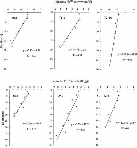
The CIC model assumes that the amount of ²¹⁰Pb_exs deposited at the sediment surface remains constant through time, that there is negligible migration of ²¹⁰Pb and associated radionuclides in the sediment, and that SARs remain constant through time. The CIC model uses age-depth relationships constructed using the ²¹⁰Pb_exs measurements and the deepest, uncompressed depth in the core above which mixing has not affected the downcore distribution of ²¹⁰Pb_exs (Figure 2). We note that some of the dated cores had visible mixing in the sediments below 28 cm, coincident with the deposition of the sand horizon below the marsh soil. Thus, even though ²¹⁰Pb_exs was detected below 28 cm, these measurements were not included in the CIC age models.

Figure 2. Downcore distribution of ²¹⁰Pb_ex in ln from the high marsh (top panels) and low marsh (bottom panels) in the western portion of Boundary Bay. Blue dots represent peat, orange dots represent silt, and red dots represent sand

The age of this deepest uncompressed depth (t, yr) was derived as:

(8) $t\left(yr\right)=-\frac{1}{\lambda }\times \mathrm{l}\mathrm{n}\left(\frac{A_x}{A_0}\right)$(8)

where A_x is the deepest ²¹⁰Pb_exs measurement, A₀ is the surface ²¹⁰Pb_exs measurement, and $\lambda$ (0.03114) is the decay constant of ²¹⁰Pb. We first plotted the natural log (ln) of the ²¹⁰Pb_exs against uncompressed depth and calculated the slope using a linear regression (Figure 2) (Callaway et al. 2012). This linear regression line was used to select points A_x and A₀ and determine the age of the sediment (Eqn 8)(8) $t\left(yr\right)=-\frac{1}{\lambda }\times \mathrm{l}\mathrm{n}\left(\frac{A_x}{A_0}\right)$(8) . Once basal ages were determined, the sediment accumulation rate (SAR, $cm/yr$) was calculated as:

(9) $SAR\left(\frac{cm}{yr}\right)=\frac{i}{t_x-t_0}$(9)

where t_x is the basal age estimated at the depth of A_x and t₀ is the age at the top of the core, and i is the uncompressed depth (cm) between the core top and A_x.

The mass accretion rate (MAR, g/cm²/yr) was calculated as:

(10) $MAR\left(\frac{g}{c{m}^{2}yr}\right)=\overline{DB{D}_i}\times SAR\left(\frac{cm}{yr}\right)$(10)

where $\overline{DB{D}_i}$ is the average DBD for samples between t_x and t_o (Table 3).

Table 3. Geochronological analyses (²¹⁰Pb dating) and carbon content were used to estimate individual core, high marsh means ±SD, low marsh means ±SD, and entire marsh means ±SD, sedimentation rates (SAR), mass accumulation rates (MAR), and carbon accumulation rates (CAR). Depth of uncompressed core represents the maximum depth at which carbon was recorded for samples that were sent for ²¹⁰Pb dating and the depth that was used to calculate SAR, MAR, and CAR

Core ID	Zone	Uncompressed core depth (cm)	Average DBD ± SD (g/cm^3)	SAR (cm/yr)	MAR (g m^-2 yr^-1)	CAR (g C m^-2 yr^-1)	Basal Age (yr)
BB1	H	18	0.451± 0.184	0.19	870 ± 355	81.8 ± 33.4	93
T3-1	H	18	0.398 ± 0.178	0.15	587 ± 263	58.6 ± 26.2	124
T2-EA (East)	H	28	0.334 ± 0.098	0.85	2843 ± 830	454.0 ±133	33
High Marsh Average ± SD	H	21 ± 6	-	0.40 ± 0.39	1433 ± 1230	198.1 ± 228.9	83 ± 46
BB2	L	17	0.911± 0.164	0.17	1554 ± 280	19.5 ± 3.5	100
LM1	L	19	0.55 ± 0.261	0.22	1184 ± 563	54.1 ± 25.7	90
T2-6 (East)	L	26	0.283 ± 0.062	0.50	1413 ± 311	151.5 ± 33.3	51
Low Marsh Average ± SD	L	21 ± 5	-	0.30 ± 0.18	1384 ± 187	75.0 ± 68.4	80 ± 25
Marsh Average ± SD	-	21 ± 5	-	0.35 ± 0.28	1408 ± 787	136.6 ± 161.6	82 ±33

H = high marsh zone; L = low marsh zone; Average DBD is calculated for samples between t_x and t_o (see Eqn 10(10) $MAR\left(\frac{g}{c{m}^{2}yr}\right)=\overline{DB{D}_i}\times SAR\left(\frac{cm}{yr}\right)$(10) and Figure 2); Stanrdard deviation on DBD is propagated to estimates of MAR and CAR.

For all cores sent for ²¹⁰Pb dating, CARs were calculated from uncompressed core depths down to the depth at which percent carbon became negligible and ²¹⁰Pb_exs activity was still detectable (Table 3). Carbon accumulation rates are calculated in two steps. First, the fraction of carbon (C_i) was estimated as the total mass of carbon divided by the total mass of the bulk sediment in each core. This fraction was estimated by summing the soil carbon densities and dry bulk densities for each depth interval:

(11) $C_i=\frac{{\sum }_0^{n}SCD\left(\frac{gC}{c{m}^3}\right)}{{\sum }_0^{n}DBD\left(\frac{g}{c{m}^3}\right)}$(11)

Second, the carbon accumulation rate (CAR, ($\frac{gC}{m^{2}yr}$)) is calculated as the product of the mass accretion rate and the carbon fraction for each core:

(12) $CAR\left(\frac{gC}{m^{2}yr}\right)=C_i\times MAR\left(\frac{g}{m^{2}yr}\right)$(12)

1.7. Statistical analysis

All data were tested for normality using the Shapiro–Wilk test for normality. T-tests were conducted to compare high and low marsh dry bulk densities, percent carbon content (%C), carbon stocks, sedimentation accumulation rates, mass accumulation rates, carbon accumulation rates, and core ages to test for any significant differences. The significance level of all the tests was set at α = 0.05. All statistical analyses were performed in R (RStudio 2015).

2. Results

2.1. Sediment properties

Depth of cores ranged from 13 to 29 cm (omitting “core” W-A as this was a pit, not a core) (Table 1). Compression occurred in most cores during field sampling due to the method used to extract cores. Compression was highest in high marsh cores and ranged between 0% and 67% (n = 6). Low marsh compression ranged between 0% and 31% (n = 4).

In all cores, weight percent of carbon (%C) was highest in the top peat layers (ranging from 2.56% to 28.05 %C) and declined with depth until the sand or silt layer was reached (Table 1; Figure A3). Sand layers contained the lowest %C values of 0.0–2.0 %C which were recorded in the bottom centimeter. In cores with no sand layer, a silt layer was found in the bottom centimeter where %C ranged from 1.7 − 10.2 %C. Only cores in the high marsh did not have sand in the deepest core layers. However, in high marsh cores, a silt layer was present before the sand layer and was considered indicative of nearing the depth of marsh initiation (Table 1; Figure A1).

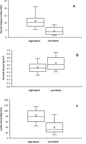
Average high marsh %C was significantly higher than average low marsh %C, at 11.3 ± 4.9 and 4.3 ± 2.6, respectively (p-value < 0.05) (Figure 3a). The average DBD in high marsh cores was 0.53 ± 0.14 g/cm³, which was not significantly different from the average DBD in low marsh cores at 0.69 ± 0.16 g/cm³ (p-value = 0.05) (Figure 3b). Soil carbon densities (SCD) for high marsh averaged 0.042 ± 0.013 g C/cm³ and were significantly higher than low marsh soil carbon densities that averaged 0.018 ± 0.008 g C/cm³ (p-value < 0.05) (Table 1; Figure A4).

Figure 3. Distribution of (a) percent organic carbon (%C), (b) dry bulk densities (g/cm³), and (c) carbon stocks (MgC/ha) for high marsh (n = 13) and low marsh cores (n = 9). The middle line is the median and the top and bottom of the box are quantiles (Q1 and Q3), the error bar is the largest and smallest value, and the x is the mean. Differences between high and low marsh are statistically significant for percent organic carbon (t-value = 3.918, p-value = 0.0004, p < 0.05) and carbon stocks (t-value = 3.602, p-value = 0.0009, p < 0.05), but insignificant for dry bulk density (t-value = −1.724, p-value = 0.050, p < 0.05)

2.2. Marsh area, carbon stocks, and accumulation rates

The western part of Boundary Bay marsh is 140 ha with high marsh accounting for 74% (103 ha) and low marsh accounting for 26% (37 ha) of marsh area (Figure 4). Comparison with the 1930 aerial photograph indicates that the western portion of Boundary Bay marsh has expanded by about 26 ha (~20%) between 1930 and 2018 (Figure 5).

Figure 4. High marsh and low marsh area in the western portion of Boundary Bay, Delta, British Columbia. High marsh (103 ha) is represented by the cross hatch fill and low marsh (37 ha) is represented by the solid fill. The green color represents area determined by variations in vegetation color using google satellite base map imagery, vegetation surveys at 176 sample points and field notes. The blue color represents area determined by variations in vegetation color using google satellite base map imagery only. Base map: Google Maps 2018

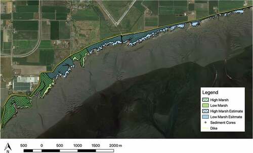
Figure 5. Marsh expansion from 1930 to 2018. (a) Air photo from 1930 was georeferenced and superimposed onto 2018 base map allowing for marsh area comparison. Base map source: NRCan, National Earth Observation data. (b) Map of the western portion of Boundary Bay salt marsh in 2018 in relation to the leading edge of the marsh in 1930. Base map source: Google Earth 2018

Average core carbon stocks for high marsh (n = 13, 83.3 ± 29.3 Mg C/ha) were significantly higher compared to average low marsh core carbon stocks (n = 9, 39.3 ± 24.2 Mg C/ha) (p < 0.05) (Figure 3c). The average carbon stocks for high marsh were still significantly higher compared to average low marsh core carbon stocks (p < 0.00001) when carbon stocks were calculated for a consistent depth horizon across all cores (compressed depth of 13 cm, which is the depth of the shortest core collected, Table 1). On average, the carbon stocks in this surface horizon (13 cm) make up 75 ± 15% of the entire organic layer of the marsh.

The entire western portion of Boundary Bay marsh (140 ha) had a total carbon stock of 10,034 ± 3,148 Mg C (traditional method), with 8,580 ± 3,018 Mg C in the high marsh (103 ha) and 1,454 ± 895 Mg C in the low marsh (37 ha) (Figure 4). For the specified bounded area where depth profiles were collected (Figure A6), the estimated carbon stocks were 2,120 ± 1,145 Mg C (traditional method) and 3,186 ± 2,269 to 3,192 ± 1,862 Mg C using the two volume-based methods (simplified and kriging approaches, respectively) (Table 2). For all three calculations of the bounded area, marsh strata were not differentiated.

SARs, MARs, and CARs exhibited high variability throughout the marsh (Table 3; Figure 6). High marsh SARs ranged from 0.15 to 0.85 cm/yr and low marsh SARs ranged from 0.17 to 0.50 cm/yr (Table 3). High marsh MARs ranged from 587 to 2843 g m⁻² y⁻¹ and low marsh MARs ranged from 1184 to 1554 g m⁻² y⁻¹. CARs ranged from 19.5 to 453.9 g C m⁻² yr⁻¹ (median = 70.1 g C m⁻² y⁻¹; average = 136.6 ± 161.6 g C m⁻² y⁻¹). No significant differences were found between the high and low marsh SARs, MARs, and CARs (all p-values > 0.05) (Table 3). High marsh CARs ranged from 58.6 to 98.4 g C m⁻² yr⁻¹ while low marsh CARs ranged from 19.5 to 151.5 g C m^-2 yr^-1.

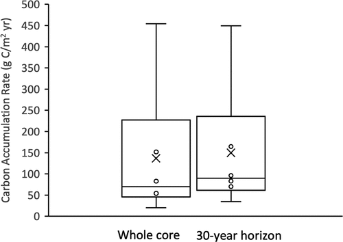
Figure 6. Carbon accumulation rates (g C m⁻² yr⁻¹) for all dated sites for the entire core and at the 30 year horizon. The middle line is the median (entire core = 70.1 g C m⁻² yr⁻¹, 30 yr = 89.7 g C m⁻² yr⁻¹), the top and bottom of the box are quantiles (Q1 and Q3), the error bar is the largest and smallest value, and the x is the mean

The basal ages of the sediment cores (depth of sand layer) ranged from 33 to 124 years, with no statistically significant difference between high and low marsh settings sampled (p = 0.464) (Table 3). High marsh cores ranged from 33 to 124 years while low marsh cores ranged from ~51 to 100 years old.

To compare the CARs for the same period of accumulation, we estimated the CARs for the last 30 years (the youngest of our dated cores) (Table A5). The results are similar to the CARs estimated for the whole cores in that no significant differences were found between the high and low marsh SARs, MARs, and CARs (all p-values > 0.05) (Figure 6, Table A5). The lack of significant differences is likely due to the high spatial variability of the marsh. However, high marsh CARs are still on average higher when compared to the low marsh CARs. Furthermore, the CARs for the last 30 years are on average 20 ± 17% higher than CARs for the entire core. Low marsh CARs were as much as 43% higher and high marsh CARs 19% higher for the 30 yr horizon compared to the entire core CARs (Table A5).

Using the median and average CARs for the marsh, we estimate that the 140 ha of the western marsh accumulates carbon at rates between 98 and 191 ± 226 Mg C/yr. If we use the average of CAR estimates for the last 30 years, this number increases to 209 ± 211 Mg C/yr.

3. Discussion

3.1. Carbon stocks

When considering the total carbon stocks in western Boundary Bay marsh, low marsh areas made up only 15% of the total carbon stock of 10,034 ± 3,148 Mg C. This lower carbon stock is likely driven by the small area and the significantly lower carbon stocks in low marsh sediment cores. Similar results were found in the Blackwater estuary, United Kingdom (Adams, Andrews, and Jickells 2012) and in the Bay of Fundy, Canada (Connor, Chmura, and Beth Beecher 2001). The high marsh typically has higher carbon storage because of deeper rooting plants, increased production of below ground biomass, and a more mature plant canopy that enables larger pieces of both in-situ and ex-situ organic matter to be stored in the soil (Connor, Chmura, and Beth Beecher 2001; Adams, Andrews, and Jickells 2012). Many studies have found that the top marsh layers have the highest amount of carbon, and carbon content declines at deeper soil depths due to diagenesis of labile material and ongoing decomposition (Adams, Andrews, and Jickells 2012; Elsey-Quirk et al. 2011; Callaway et al. 2012; Jensen et al. 2006; Patrick Jr. and DeLaune 1990).

This result could have implications for the engineering of a living dike. For example, the expansion of low-marsh zones with patchy low-marsh vegetation and shallower root systems could be less stable and less likely to hold large amounts of carbon. This is especially concerning when taken with the potential for marsh edge erosion due to sea-level rise (Kirwan et al. 2016; FitzGerald and Hughes 2019). Buildup of carbon may depend on development of a mature, dense plant canopy that can trap and store more in-situ and ex-situ carbon (Best et al. 2018), although other research suggests that even densely vegetated marsh areas are prone to channel development and associated erosion (Temmerman et al. 2007). In terms of carbon, our results imply that marsh enhancement would need substantial components of high marsh to maximize a carbon co-benefit. Thus, the development of sediment elevation suitable to mid and high marsh vegetation will be essential to maximize blue carbon sequestration and storage.

Our core carbon stocks of 39.3 ± 24.2 Mg C/ha for low marsh and 83.3 ± 29.5 Mg C/ha for high marsh are lower than the estimated global carbon stock of 250 Mg C/ha (Chmura et al. 2003; Pendleton et al. 2012). The leading reason for this difference is that the global estimate was calculated for the top meter of soil (Duarte et al. 2013) while our carbon stocks only reached depths of refusal of 21–70 cm (mean of 32 ± 16 cm), which is considered marsh initiation. Our shallow depths may simply indicate a younger marsh (Shepperd 1981), in which the depths of refusal ranged from 33 to 124 years old. Sedimentological studies also suggest that the current marsh is underlain by a sandy gravel beach-ridge complex (Engels and Roberts 2005; Dashtgard 2011). Our results support this assumption because in the nine cores that have a distinct bottom sand layer, six of them have no carbon recorded in the sand layer (Figures A1 and A4, Table A4). Notably, Crooks et al. (2014) found similar carbon stocks of 71.7 Mg C/ha and 53.7 Mg C/ha for the top 30 cm of two marshes in the nearby Snohomish Estuary, Washington.

If we were to extrapolate our carbon stocks to 1 m (multiplying the average uncompressed SCDs of low and high marsh samples by 1 m), the carbon stocks for Boundary Bay would be 140 ± 60 Mg C/ha and 284 ± 140 Mg C/ha for the low and high marsh, respectively. These extrapolated high marsh values align closely with the global average while the low marsh stocks are still substantially lower. Our mean uncompressed SCD of 0.024 ± 0.014 g/cm³ (for both high and low marshes) is slightly lower but still within range of the global salt marsh SCD mean of 0.039 ± 0.003 g/cm³ (Chmura et al. 2003). Only limited carbon stock data from the Pacific coast of North America have been included in global syntheses (Chmura et al. 2003; Ouyang and Lee 2014), and most data are from the Atlantic coast of North America and the Gulf of Mexico. Thus, the “global” estimate is skewed toward regions that may have marsh depths of 1 m or deeper, are older in age, have different geological processes, and have different climate and vegetation assemblages.

Our extrapolated results indicate that if the marsh’s organic carbon layer were to become deeper with age, Boundary Bay marsh could compare to the global average. The oldest marsh ages in Boundary Bay indicate that the current marsh has only been accumulating for 33–124 years (Table 3). Thus, one might expect that any carbon co-benefits of a living dike structure will be measured over longer (decadal-to centennial) rather than shorter (annual) time scales.

Our discussion above indicates that extrapolating salt marsh carbon stocks to a fixed depth can substantially overestimate regional carbon stocks, in particular for marshes with depths of marsh initiation shallower than the reference horizon of 1 meter. For this study, we undertook a novel sensitivity test of two new volumetric approaches that might provide more accurate estimates of marsh carbon content. To our knowledge, no other study considers the volume of the marsh when calculating carbon stock (Howard et al. 2014; Connor, Chmura, and Beth Beecher 2001; Elsey-Quirk et al. 2011). Our sensitivity test indicates that the method for calculating carbon stock can influence the final estimate of carbon stored, but the spatial variability in marsh characteristics imparts an uncertainty that is comparable in magnitude to the differences between methods. Specifically, the volumetric-based methods estimated carbon stocks that were 35% higher than the traditional method (Table 2). However, uncertainties in our estimates are larger than the differences between methods, ranging from ± 54% (traditional method) to 58% (kriging volume) to 71% (simplified volume). The uncertainties in these calculations can be attributed to several factors, including spatial variability in (a) carbon stocks calculated for each core $\overline{Cstoc{k}_{core}}$ (SD ± 54%); (b) estimated depths of refusal $Z_{core}$ (SD ± 41%), and (c) uncompressed SCDs (SD ± 58%). Additional factors, such as assuming a constant compression factor when uncompressing core depths, contribute further to this uncertainty, although their values are not known. We note, however, that assuming global C stock estimates (250 Mg C/ha) and accumulation to a depth of 1 m would substantially overestimate the carbon stocks, resulting in a value of 8115 Mg C for the bounded area (more than 2.5 times greater than our highest estimate).

3.2. Carbon accumulation rates

While high marsh carbon stocks are substantially greater than those in the low marsh, our CARs do not show any significant differences between high and low marsh, for either the entire core or the 30-yr horizon CARs. Boundary Bay marsh exhibits strong spatial variability in accumulation rates, ranging from 19.5 to 454.0 g C m⁻²yr⁻¹ (Table 3; Figure 6). The average CAR of 136.6 ± 161.6 g C m^-2 yr^-1 is clearly skewed by the high marsh core T2-EA (CAR of 454.0 g C m^-2yr^-1). Due to the financial limitations of this study, we have not dated enough cores throughout the marsh to indicate if high CARs are localized or representative of a larger area of the marsh. However, because all other cores are in the range of 19.5–151.5 g C m^-2yr^-1, the median of the CARs (70.1 g C m^-2yr^-1) may be a more appropriate indicator of the CAR in the western portion of Boundary Bay. The median is also similar to the average CAR (73.1 ± 49.1 g C m^-2yr^-1) when T2-EA is omitted.

The median (70.1 g C m^-2yr^-1) and average (136.6 ± 161.6 g C m^-2yr^-1) CARs in western Boundary Bay marsh are similar to other marshes on the Pacific coast of North America. Callaway et al. (2012) reported an average CAR of 79 g Cm^-2yr^-1 for four salt marshes and two brackish marshes in San Francisco Bay and similarly found no significant differences between high and low marsh. In the Snohomish Estuary in Washington, USA, the natural saline marsh on which ²¹⁰Pb dates were measured (Quilceda Marsh) had CARs of 110.2 g C/m^-2 yr^-1 (Crooks et al. 2014), while CARs in Clayoquot Sound, BC, average 115 ± 34.2 g C m^-2yr^-1 (Chastain et al. manuscript in preparation). Notably, these estimates are all substantially lower than global estimates of 244.7 ± 26.1 g C m^-2yr^-1 (Ouyang and Lee 2014).

While our study found no significant differences between high marsh and low marsh CARs, the higher percent carbon, higher soil carbon densities, and higher carbon stocks in high marsh sediments indicates that the high marsh may have a greater ability to accumulate carbon compared to the low marsh. In nearby Clayoquot Sound, BC, high marsh sites had significantly higher CARs when compared to low marsh CARs (Chastain et al. manuscript in preparation). In contrast, studies from the east coast of North America find that low marsh cores have significantly higher CARs (Elsey-Quirk et al. 2011; Connor, Chmura, and Beth Beecher 2001; Ouyang and Lee 2014). This difference may be driven partially by vegetation type, which can contribute varying qualities and quantities of litter to sediments (Zhou et al. 2006; Mahaney, Smemo, and Gross 2008; Kelleway et al. 2017). Elsey-Quirk et al. (2011) found that Spartina alterniflora dominated the low marsh and had a CAR of 154 g C m⁻²yr⁻¹, and Juncus roemerianus dominated the high marsh and had a CAR of 119 g C m⁻²yr⁻¹. Ouyang and Lee (2014) found that among five halophyte genera, Spartina spp demonstrated the highest capacity for carbon accumulation. In contrast to many east coast sites, the low marsh sites in Boundary Bay were dominated by Salicornia virginica and Triglochin martima, and Spartina spp were absent. Kelleway et al. (2017) found that Salicornia spp. had a lower carbon deposition and lower ability to retain and preserve organic inputs compared to Juncus spp.

The difference in vegetation structure has implications for potential future carbon sequestration of a living dike structure in Boundary Bay. Many Spartina species are classified as invasive in BC and are being actively managed (BC Spartina Working Group 2016). Controls on Spartina spp. are designed to keep them from colonizing the low marsh and displacing the dominant Salicornia spp. We anticipate that the living dike expansion of low marsh zones with Salicornia spp. will increase carbon accumulation rates overall, but at lower rates than in ecosystems dominated by Spartina spp, and therefore will have lower CARs than recorded elsewhere. Knowing the vegetation composition will be important to projecting how CARs are likely to increase.

As stated above, Boundary Bay marsh is relatively young, with basal ages from 33 to 124 years old. We are therefore able to measure the CARs from various marsh initiation points throughout the marsh and provide valuable information of how the marsh has accumulated carbon over time (Table 3; Table A5). Most studies have not indicated that they reached the point of marsh initiation and therefore must choose a constant horizon at which to compare rates (Elsey-Quirk et al. 2011; Callaway et al. 2012; Crooks et al. 2014). Estimating CARs for a 30-yr marker horizon allows us to compare CARs across the marsh for a consistent time period, but also to examine how CARs differ between marsh initiation and the most recent 30 years (Figure 6). Specifically, CARs average 20 ± 17% higher during the last 30 years than for the entire core, likely due to higher carbon concentrations in the upper layers of the marsh (Figure A3 and A4). If only measuring CARs from a relatively young horizon marker, researchers may overestimate the overall long-term ability of the marsh to accumulate carbon.

3.3. Marsh processes and expansion

Salt marshes are complex systems which exhibit spatial variability in depositional rates (Chmura, Coffey, and Crago 2001; Fagherazzi et al. 2012), and our analysis indicates that Boundary Bay is no exception. Two cores collected further east, low marsh core T2-6 and high marsh core T2-EA, have higher SARs and CARs than cores collected further west (Table 3). Tidal range, sediment supply, elevation, proximity to tidal channels, and vegetation assemblages can all contribute to this spatial variability in deposition (Roner et al. 2016; Van De Broek et al. 2018; Kelleway et al. 2017; Fagherazzi et al. 2012; Temmerman et al. 2005). In Boundary Bay, a large and deep tidal channel runs east-west across the eastern portion of the marsh and may contribute to more frequent flooding, different water velocities, and greater amounts of sediment and carbon deposition.

The marsh further east also appears to be younger, which may contribute to its higher CARs. Callaway et al. (2012) found that younger sites exhibit higher CARs than older, established marshes because stored carbon had not decomposed. As marshes age, the soils naturally lose some of the carbon in outflow waters as well as through slow rates of decomposition (Callaway et al. 2012; Villa and Bernal 2018). The eastern portion of the marsh tends to be deeper, which suggests that natural compaction of the soils has not yet taken place (Figure A6) (Allen 1999).

Higher CARs in the eastern part of the study area may also be indicative of the marsh’s historical response to human alterations and disturbances over the past 150 years. In the 1880s, farmers began protecting farmland from flooding by diking the northern part of the marsh. After the great flood of 1948, the City of Delta reinforced the dike along Boundary Bay (Shepperd 1981), and it serves as the landward boundary of the marsh today. The marsh has also experienced modifications to freshwater inputs, disturbances, and sedimentation (Boyle et al. 1997). The 1930 air photo shows a small creek to the northeast of the cores T2-6 and T2-EA which no longer exists today (Figure 5). Studies of Boundary Bay in the 1960s and 1970s suggest that the rise of the logging industry in BC resulted in increased disturbances from logs washing up and rafting over the marsh surface (Kellerhalls and Murray 1969; Porter 1982). Dredging of the Serpentine and Nikomekl Rivers in the far east of Boundary Bay, dredging of the Fraser River, and upstream deforestation may all have altered sediment supply over the years (Boyle et al. 1997).

Despite historical modification of the marsh, the western portion of the Boundary Bay marsh is growing (Figure 5). Marsh expansion is a rare event in coastal marshes and is usually due to anthropogenic land changes and accumulation of debris from hydraulic mining (Watson 2008). Kellerhals and Murray (1969) hypothesized that western Boundary Bay marsh is prograding in response to tidal influence, sedimentation and vegetation growth, and ecological interactions that influence the growth of hummocks and eventual cohesion with the marsh. They surmised that the large quantities of eelgrass and algae are rafted onto hummocks and then covered with sand from strong winter storms. The new relief is then colonized with blue-green algal mats which then allow for typical sediment trapping and eventual halophyte propagation. The farthest western portion of the marsh contains a large beach ridge that was not present in the 1930s (Figure 5 and A6) (Engels and Roberts 2005). The area contained large logs and flotsam that blocked a large channel and has since been overgrown by vegetation (Kellerhalls and Murray 1969).

One interesting question is how much this 26-ha marsh expansion could have contributed to additional carbon storage since the 1930s. A simple calculation using the average carbon stock (65.3 ± 35.3 Mg C/ha) suggests that expansion may have added 1,698 ± 918 Mg C, at a rate of approximately 20 Mg C/y over 85 years. If we calculate carbon accumulation for the same 85-year period using the median CAR (70.1 g C/m²/yr), we gain a similar result of 1,549 Mg C (18 Mg C/yr). The average CAR (136.6 ± 161.6 g C/m²/yr) produces a higher estimate of 3,028 Mg C (or 36 Mg C/yr), but obviously with a substantially larger uncertainty (± 3,582 Mg C). The similarity between the estimates using the average carbon stocks and median CAR suggest that the likely range is 1,549–1,698 Mg C, or 18–20 MgC/y. Nevertheless, the high spatial variability in our marsh carbon accumulation rates underscores the uncertainties with this calculation.

Our analysis of historical marsh development has implications for the monitoring and long-term development of carbon sequestration in Boundary Bay especially with future inclusion of a living dike structure. First, the monitoring of carbon sequestration as part of a living dike plan may be challenging if the plan is to create islands of marsh that will eventually grow together; this plan is likely to increase the spatial heterogeneity of high- and low-lying areas, leading to spatially variable accumulation rates like the ones calculated above. Thus, monitoring will be required to sample different geomorphological types and marsh ages. Second, there also needs to be a cautious approach regarding initially high sequestration rates in young, high marsh areas, as these are likely to overestimate overall, long-term accumulation rates. Ultimately, a comprehensive assessment of marsh dynamics will require additional knowledge of processes in the east and central parts of Boundary Bay where evidence has been found of marsh degradation (Dashtgard 2011; Engels and Roberts 2005; Kellerhalls and Murray 1969). Understanding these sediment transport dynamics will be essential to the strategic design and emplacement of a living dike structure.

3.4. Blue carbon and climate change mitigation

Previous studies have suggested that the quantification of a salt marsh’s blue carbon potential can be used to prioritize restoration efforts, as well as support management decisions that help communities adapt to climate change and mitigate greenhouse gas emissions (Duarte et al. 2013; Sheehan et al. 2019). For example, restoration efforts can be prioritized for areas that allow marsh migration into agricultural or rural areas near the coast, to increase salt marsh area, and reduce the threat of coastal squeeze (Elsey-Quirk et al. 2011; Temmerman et al. 2013; Schuerch et al. 2018). In areas where hard barriers cannot be removed, applying living shoreline management and restoration techniques can be used to enhance the resiliency of a marsh in the face of sea-level rise (Temmerman et al. 2013; Sheehan et al. 2019).

In Boundary Bay, this study demonstrates that the western part of the marsh has a significant carbon stock that continues to accumulate carbon every year and can be deemed a local hot spot for carbon storage and accumulation. However, marsh sediments elsewhere in Boundary Bay may not keep pace with sea-level rise or may already be eroding. Understanding the dynamics of sediment transport, as well as the incorporation of sea-level models, will be essential to creating a successful blue carbon sequestration and storage function to the living dike. Attention to the development of dike elevations suitable to mid and high marsh vegetation will be essential to maximize blue carbon sequestration and storage.

3.5. Valuing blue carbon

Incorporating BC salt marshes into carbon offset initiatives could also offer a valuable backstop for ecosystem protection by providing a new lens through which to view their importance, and by engaging local governments, businesses, and the general public. The benefits of incorporating salt marshes into offset/credit systems calls attention to the economic importance of their carbon sequestration services and raises the political agenda to support blue carbon initiatives and policy (Ullman, Bilbao-Bastida, and Grimsditch 2013). Additionally, these offsetting/credit programs could provide direct protection as well as ongoing funding for the conservation, restoration, and monitoring of these ecosystems (Luisetti, Jackson, and Turner 2013; Vanderklift et al. 2019).

However, the inclusion of salt marshes into offsetting initiatives, or the management of natural carbon sinks more generally, will be difficult with the current state of research, policy design, economic analysis, and policy advocacy (Ullman, Bilbao-Bastida, and Grimsditch 2013). Our study provides a first step in documenting the baseline of carbon sequestration processes in Boundary Bay, but on-going monitoring, reporting, and maintenance of a project and its carbon potential (sequestration and stock) would be required (Emmer et al. 2015; Watson et al. 2000). There are also significant issues related to governance and jurisdiction of salt marshes, and of coastal ecosystems in BC more broadly, that need to be considered, including the inherent jurisdiction and constitutionally protected title and rights of Indigenous Peoples (The Constitution 1982), and the implementation of the United Nations Declaration on the Rights of Indigenous Peoples (United Nations 2011; Declaration 2019).

Based on our research and experiences, future research should involve: (a) quantification of other BC salt marsh CARs and carbon stocks, (b) a full understanding of marsh specific carbon budgets, including potential GHG emissions; and (c) modeling and mapping to determine marsh persistence into the future. This research may take several years to complete, and therefore salt marsh inclusion in potential offsetting initiatives in BC is still some years away. Nonetheless, this ecosystem valuation mechanism has potential as a robust and efficient way of supporting the sustainability of salt marshes and their carbon mitigation abilities in the future (Ullman, Bilbao-Bastida, and Grimsditch 2013).

3.6. Next steps

While this study has led to an improved understanding of marsh processes in western Boundary Bay, additional research is needed to incorporate Boundary Bay marsh as a carbon co-benefit for green infrastructure or as part of any carbon accounting scheme. These research steps include determining: (1) allochthonous and autochthonous carbon composition in the sediment, (2) permanency of the marsh in relation to projected sea level rise, and (3) the greenhouse gas budget and marsh topography of the entire Boundary Bay marsh.

First, understanding the contributions of allochthonous and autochthonous carbon is essential for avoiding the overestimation of marsh carbon sequestration and the “double accounting” of ex-situ carbon from neighboring ecosystems (Macreadie et al. 2019; Van De Broek et al. 2018). Most estimated carbon stocks and accumulation rates are based on the assumption that the organic carbon stored in the marsh is autochthonous (Van De Broek et al. 2018), which can result in an overestimation of overall carbon sequestration (Van De Broek et al. 2018; Macreadie et al. 2019). In reality, salt marshes have a combination of allochthonous terrestrial and oceanic organic matter inputs, as well as autochthonous carbon produced by above and below ground macrophyte litter (Zhou et al. 2006; Van De Broek et al. 2018). The amount of external inputs into the marsh depends on several factors, such as catchment area size, land-use, and the duration of exposure to ocean waters, which differs between marshes (Gillis et al. 2014). In addition to carbon and nitrogen isotope tracers, n-alkane distributions, C/N elemental ratios, lignin, lipids, and amino acid biomarkers can help determine carbon sources in salt marsh sediments (Kumar et al. 2020; Zhou et al. 2006; Tanner et al. 2010; Canuel and Hardison 2016; Bianchi et al. 2011; Macreadie et al. 2019). In the case of Boundary Bay marsh, carbon contributions are anticipated from in-situ marsh production, but also riverine sources from the east, outflow from farmland, terrestrial inputs from nearby Roberts Point, as well as oceanic sources. Ultimately, accounting for the appropriate amount and source of carbon within the marsh will allow for greater confidence in including Boundary Bay marsh in carbon accounting/credit programs.

Another important analysis for Boundary Bay salt marsh is the detailed mapping of marsh elevation to understand its resiliency to future sea level rise. Salt marshes are threatened by sea level rise if they do not have space to migrate inland or accretion rates that exceed projected sea level rise (Mcleod et al. 2011; Chmura 2013). Assessing whether a salt marsh will persist into the future is essential for verifying if the site is appropriate for a greenhouse gas offset credit or program (Chmura 2013; Macreadie et al. 2019). If a marsh is drowned and permanently lost, then the carbon stored in the marsh will be released into the atmosphere, contributing to greenhouse gas emissions (Duarte et al. 2013; Sheehan et al. 2019). While digital elevation models infer elevations of land close to sea level (Amante 2018), most are too coarse to provide accurate estimates of marsh elevation within centimeters (Chmura 2013; Kulp and Strauss 2019). Topographic Lidar could provide digital elevation models with vertical resolution relevant to marshes and would help determine the permanency of Boundary Bay marsh – and its blue carbon – in relation to projected sea level rise (Chmura 2013).

Finally, investigations of the greenhouse gas budget and a comprehensive survey of the entire marsh are still needed. Poffenbarger, Needelman, and Patrick Megonigal (2011) found that polyhaline marshes (salinity > 18) have negligible amounts of methane emissions, whereas fresh (salinity = 0–0.5) and mesohaline (salinity = 5–18) marshes have variable methane emissions that could emit more methane than carbon being stored. Although Boundary Bay has a salinity range of 24 to 29 at the leading edge of the marsh (Swinbanks et al. 1981) and the vegetation assemblage suggests that the marsh on a whole has a salinity greater than 18 (Porter 1982; Weinmann et al. 1984), further investigation of porewater salinities is needed to ensure Boundary Bay salt marsh is a carbon sink. A comprehensive sampling of porewater salinity and quantification of methane fluxes throughout the entire marsh would allow for greater certainty in the carbon sequestration (Poffenbarger, Needelman, and Patrick Megonigal 2011). Similar quantification of greenhouse gas budgets (as well as vegetation, extent, salinity, and carbon dynamics) are required in the ~85 ha of marsh in the eastern portion of Boundary Bay, as well as the marshes found in the far east in Mud Bay.

In conclusion, this study provided the first quantification of carbon storage and accumulation rates in the high and low marsh zones of the western portion of the Boundary Bay salt marsh in Delta, British Columbia, thus contributing to the estimation of blue carbon potential on the Pacific Coast of Canada. This study also provides an essential first step in understanding the carbon dynamics of Boundary Bay marsh prior to the initiation of living dike solutions designed to protect against sea-level rise. To ensure the marsh continues to sequester and store carbon, especially with the implementation of engineered living dike structures, we recommend that on-going monitoring, such as erosion, sea level rise, and species composition of the marsh, will be needed. If Boundary Bay marsh were to be incorporated into an offsetting initiative or other carbon management program in British Columbia, all of these steps, including determining the composition of the allochthonous and autochthonous carbon and the measuring of elevation, would need to be completed to have a robust and comprehensive baseline of carbon sequestration in Boundary Bay.

Acknowledgments

We are very grateful to B. Galeb (University of Quebec at Montreal) for assistance and expertise with ²¹⁰Pb analysis, and M Soon (UBC) for technical assistance with elemental analysis, and three anonymous reviewers who greatly improved the manuscript. Assistance with fieldwork, laboratory work, and data support was provided by S. Murphy, J. Morra, N. Mohr, S. Chastain, V. Postlethwaite, J. Jones, and I. Sukse. Parks Canada provided in-kind and logistical support for laboratory and field analysis. This project was funded by a Mitacs Accelerate grant awarded to KEK and MG, jointly funded by Canadian National Science and Engineering Research Council (NSERC) and West Coast Environmental Law; NSERC [Discovery Grant RGPIN342251] to KEK; NSERC Canada Research Chair Award to KEK, and several SFU scholarships and awards to MG (VanCity Environmental Graduate Scholarship, Travel and Minor Research Award, Graduate Fellowship, and a Special Graduate Entrance Scholarship).

Disclosure statement

The authors have no potential competing interests.

Additional information

Funding

This work was supported by a grant from the Mitacs Accelerate Program and West Coast Environmental Law to KEK and MG; the National Science and Engineering Research Council [RGPIN342251] to KEK; and a Canada National Science and Engineering Research Council Canada Research Chair to KEK.

Appendix A.

Supplemental Figures and Tables

Figure A1. Soil horizons of each core sampled in summer 2017 and summer 2018 in relationship to length of core (cm) (n = 14). Dark gray represents wood, brown represents sand, dark blue represents sand and peat mix, dark green represents silt and sand mix, yellow represents silt, light blue represents peat and silt mix, and green represents the top peat layer. Core W-A was not a core, but a pit with soil samples taken every 5 cm. All cores are shown with compressed depths

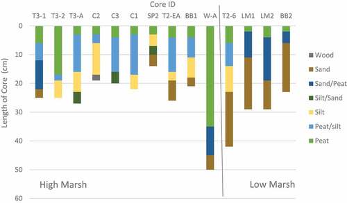
Figure A2. Percent total carbon (EA) to percent loss-on-ignition (LOI) least-squares regression relationship. Percent total carbon calculated using elemental analyzer data from this study (BB1 and BB2) and EA and LOI data from Chastain (2017), whose data is calculated from cores sampled in marshes in Clayoquot Sound, British Columbia

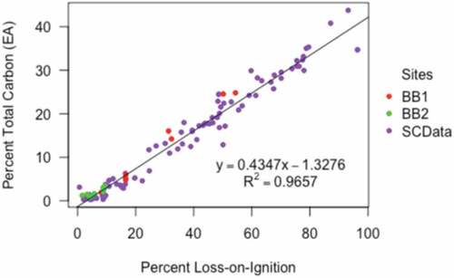
Figure A3. Profiles of sediment percent carbon (%C) for each core in relationship to depth of each core (cm). Red dotted lines represent high marsh cores and blue dotted lines represent low marsh cores

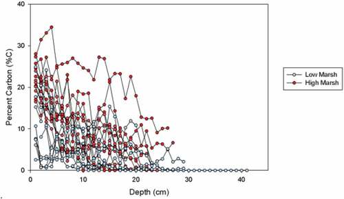
Figure A4. Profiles of sediment soil carbon densities (g C/cm³) for each core in relationship to depth of each core (cm). Red dotted lines represent high marsh cores and blue dotted lines represent low marsh cores

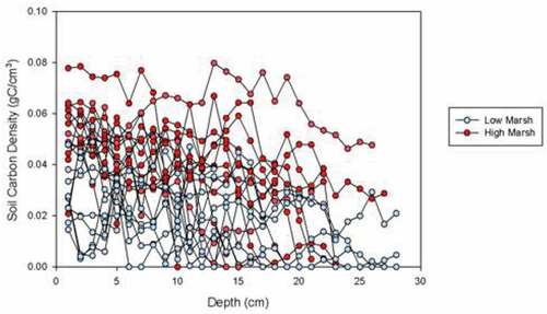
Figure A5. Marsh zonation with specific vegetation distributions in relation to collected cores in the western portion of Boundary Bay. Base Map Source: Google Earth 2018. Base Data. Source: QGIS 3.0

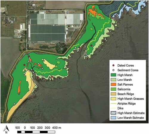
Figure A6. The kriging spatial analysis completed in ArcMap 10.3 to estimate the marsh volume based on the bounded area. Surface elevation is measured in meters. Base map source: Google Earth 2018

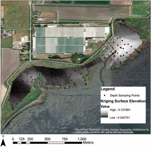
Table A1. Sediment core sampling information collected in the western portion of Boundary Bay, Delta, BC. Core W-A was not a core, but a pit with soil samples taken every 5 cm. The core length represents the length of the core once extracted from the core, and the depth of refusal represents the depth of the core hole once the core had been extracted (length of core penetration)

Core ID	Latitude 49 –	Longitude 123 02’ –	Date Collected Summer -	Marsh Zonation	Core Length	Depth of Refusal	Soil Type at Bottom of Core
T3 - 2	02’ 50.1”	45.2”	2018	HM	25	75	Silt
T3 - A	02’ 49.1”	48.8”	2018	HM	27	52	Silt/Sand
C2	02’ 54.4”	46.1”	2018	HM	19	n/a	Woody Debris
C3	02’ 53.2”	39.4”	2018	HM	20	25	Silt/Sand
BB1	02’ 55.6”	44.6”	2017	HM	21	21	Sand
BB1-4	02’ 55.7’’	45.5’’	2014	HM	18	n/a	Unknown
BB1-3	02’ 50.7’’	43.9’’	2014	HM	24	n/a	Unknown
BB2-5	03’ 00.2’’	15.3’’	2014	HM	24	n/a	Unknown
T2-EA	03’ 01.1”	04.9”	2018	HM	27	50	Sand
W-A	02’ 36.2”	55.3”	2018	HM	45*	45 (pit)	Sand
C1	02’ 54.4”	44.5”	2018	S	21	n/a	Silt
SP2	02’ 51.1”	37.0”	2018	S	16	23	Sand
T3 - 1	02’ 52.8”	48.7”	2018	HM	25	35	Sand
BB1 - 2	02’ 49.6’’	42.9’’	2014	LM	29	n/a	Unknown
BB2	02’47.6”	40.0”	2017	LM	23	23	Sand
BB1 - 1	02’ 44.0’’	40.8’’	2014	LM	17	n/a	Unknown
BB2 - 4	02’ 59.1’’	13.4’’	2014	LM	19	n/a	Unknown
BB2 - 3	02’ 57.4’’	08.3’’	2014	LM	13	n/a	Unknown
BB2 - 2	02’ 56.9’’	07.6’’	2014	LM	20	n/a	Unknown
T2 -6	03’ 00.1”	12.6”	2018	LM	42	60	Sand
LM1	02’ 47.7”	30.6”	2018	LM	29	40	Sand
LM2	01’ 48.0”	36.6”	2018	LM	29	42	Sand

HM = high marsh; LM = low marsh; S = salt panne; * pit

Table A2 Species composition and marsh zonation of coring sites in Boundary Bay, Delta, BC. Sites were considered (a) low marsh if the dominant plant species were Salicornia virginica, Triglochin martima, and Spergularia marina (Porter 1982; Weinmann et al. 1984); (b) high marsh if the dominant plant species were Atriplex patula, Distichlis spicata, Grindelia integrifolia, Aster subspicatus, Deschampsia cespitose, Scirpus maritimus, and Achillea millefolium (Porter 1982; Weinmann et al. 1984). Salicornia virginica was found across both strata, but it was most prevalent in the low marsh.

Core ID	Species	Percent Cover	Marsh Zonation
BB1-1	Jaumea	<1%	Low Marsh
	Salicornia	95%
	Triglochin	<1%
	Atriplex	2%
BB1-2	Salicornia	75%	Low Marsh
	Atriplex	25%
BB1-3	Atriplex	99%	High Marsh
	Salicornia	>1%
BB1-4	Distichlis	98%	High Marsh
	Atriplex	>1%
	Salicornia	>1%
BB2-2	Salicornia	70%	Low Marsh
	Atriplex	30%
	Deschampsia	<1%
BB2-3	Salicornia	85%	Low Marsh
	Atriplex	15%
BB2-4	Salicornia	60%	Low Marsh
	Distichlis	20%
	Atriplex	20%
BB2-5	Atriplex	70%	High Marsh
	Distichlis	30%
BB – 1	Salicornia	20%	High Marsh
	Deschampsia	5%
	Grindelia	10%
	Distichis	25%
BB – 2	Salicornia	50%	Low Marsh
	Triglochin	25%
	Juncus	25%
C1	Salicornia	-	High Marsh (salt panne)
	Dead Salicornia	97%
	Live Salicornia	3%
C2	Grindelia	30%	High Marsh
	Elymus	45%
	Atriplex	2%
	Distichlis	10%
	Achillea	2%
C3	Juncus	99%	High Marsh
	Salicornia	1%
T3-1	Salicornia	40%	High Marsh
	Grindelia	40%
	Distichlis	20%
T3-2	Achillea millefolium	25%	High Marsh
	Elymus	45%
	Solidago	5%
	Atriplex	20%
T3 -A	Atriplex (dead)	80%	High Marsh
	Salicornia	20%
T2 -EA	Atriplex	50%	High Marsh
	Salicornia	25%
	Distichlis	15%
	Grindelia	10%
T2 − 6	Triglochin	45%	Low Marsh
	Salicornia	25%
	Distichlis	25%
	Atriplex	5%
LM1	Salicornia	95%	Low Marsh
	Atriplex	5%
LM2	Salicornia	95%	Low Marsh
	Distichlis	5%
SP2	Salicornia	2%	High Marsh (salt panne)
	Bare ground	98%
W-A	Distichlis	100%	High Marsh

Table A3. Coordinates, species composition, and depth of organic layer of 154 additional sampling sites in Boundary Bay, Delta, BC. Twenty-seven transects separated every 50 m were selected, and each sampling site was approximately every 50 m in each transect. Of the 154 additional sampling sites, 139 depth measurements were collected by pushing a metal meter stick one meter in length into the ground until sand was hit

Latitude	Longitude	Species Composition	Depth (cm)
N 49° 02’36.6”	W 123° 02’55.6”	Scirpus maritimus	23
N 49° 02’36.7”	W 123° 02’55.8”	Distichlis spicata	51
N 49° 02’37.6”	W 123° 02’55.8 “	Atriplex patula	38
		Scirpus maritimus
N 49° 02’38.4”	W 123° 02’56.2”	Scirpus maritimus	47
N 49° 02’39.5”	W 123° 02’56.7”	Scirpus maritimus	n/a
N 49° 02’40.5”	W 123° 02’57.6”	Distichlis spicata	30
N 49° 02’43.3”	W 123° 02’56.7”	Distichlis spicat0a	30
N 49° 02’41.7”	W123° 02’55.8”	Distichlis spicata	28
N 49° 02’40.2”	W 123° 02’55.0”	Achillea millefolium	34
		Distichlis spicata
N 49° 02’38.6”	W 123° 02’53.7”	Distichlis spicata	48
N 49° 02’40.1”	W 123° 02’51.6”	Distichlis spicata	45
N 49° 02’40.3”	W 123° 02’51.8”	Salicornia virginica	35
		Distichlis spicata
N 49° 02’41.1”	W 123° 02’52.4”	Salicornia virginica	30
N 49° 02’41.6”	W123° 02’53.0”	Salicornia virginica	30
N 49° 02’43.4”	W 123° 02’53.6”	Distichlis spicata	30
		Achillea millefolium
N 49° 02’45.5”	W 123° 02’54.5”	Distichlis spicata	25
N 49° 02’49.0”	W 123° 02’55.6”	Scirpus maritimus	20
		Salicornia virginica
N 49° 02’49.2”	W 123° 02’55.1”	Distichlis spicata	30
N 49° 02’47.7”	W 123° 02’53.5”	Distichlis spicata	30
		Atriplex patula
N 49° 02’47.2”	W 123° 02’53.1”	Salicornia virginica	20
N 49° 02’46.6”	W 123° 02’52.7”	Salicornia virginica	20
		Atriplex patula
N 49° 02’45.5”	W 123° 02’52.0”	Salicornia virginica	30
N 49° 02’45.2”	W 123° 02’51.7”	Bare soil	7
N 49° 02’42.2”	W 123° 02’49.4”	Distichlis spicata	35
		Achillea millefolium
N 49° 02’44.2”	W 123° 02’47.7”	Distichlis spicata	40
N 49° 02’46.3”	W 123° 02’48.9”	Distichlis spicata	45
N 49° 02’46.3”	W 123° 02’48.9”	Grindelia integrifolia	20
		Salicornia virginica
		Distichlis spicata
N 49° 02’47.5”	W 123° 02’50.0”	Salicornia virginica	30
		Grindelia integrifolia
N 49° 02’47.8”	W 123° 02’49.9”	Grindelia integrifolia	n/a
		Distichlis spicata
		Salicornia virginica
N 49° 02’49.3”	W 123° 02’50.8”	Distichlis spicata	35
N 49° 02’49.4”	W 123° 02’50.7”	Grindelia integrifolia	n/a
		Salicornia virginica
N 49° 02’51.6”	W 123° 02’51.6”	Distichlis spicata	25
		Grindelia integrifolia
		Salicornia virginica
N 49° 02’53.0”	W 123° 02’52.1”	Distichlis spicata	32
N 49° 02’55.1”	W 123° 02’49.3”	Aster subspicatus	30
		Grindelia integrifolia
		Distichlis spicata
N 49° 02’53.7”	W 123° 02’48.6”	Grindelia integrifolia	25
		Distichlis spicata
		Salicornia virginica
N 49° 02’53.7”	W 123° 02’48.6”	Salicornia virginica	30
N 49° 02’51.8”	W 123° 02’47.7”	Grindelia integrifolia	n/a
		Salicornia virginica
		Atriplex patula
N 49° 02’51.1”	W 123° 02’47.0”	Atriplex patula	60
		High marsh grasses
N 49° 02’51.1”	W 123° 02’47.1”	Atriplex patula	58
		Achillea millefolium
N 49° 02’49.9”	W 123° 02’46.4”	Atriplex patula	60
		Achillea millefolium
		Aster subspicatus
		Distichlis spicata
N 49° 02’48.9”	W 123° 02’46.6”	High marsh grasses	45
N 49° 03’29.3”	W 123° 01’23.6”	Salicornia virginica	8
		Atriplex patula
		Distichlis spicata
		Juncus roemerianus
N 49° 03’29.6”	W 123° 01’22.8”	Juncus roemerianus	3
		Salicornia virginica
		Triglochin martima
N 49° 03’31.6”	W 123° 01’22.6”	Juncus roemerianus	24
		Salicornia virginica
		Grindelia integrifolia
N 49° 03’34.3”	W 123° 01’20.0”	Atriplex patula	23
		Salicornia virginica
N 49° 03’34.4”	W 123° 01’15.9”	Distichlis spicata	30
		Salicornia virginica
		Atriplex patula
N 49° 03’33.1”	W 123° 01’13.0”	Atriplex patula	40
		Grindelia integrifolia
		Salicornia virginica
N 49° 03’31.5”	W 123° 01’14.5”	Atriplex patula	36
N 49° 03’30.4”	W 123° 01’15.7”	Atriplex patula	32
		Salicornia virginica
N 49° 03’29.7”	W 123° 01’17.8”	Atriplex patula	37
		Salicornia virginica
		Grindelia integrifolia
		Triglochin martima
N 49° 03’23.8”	W 123° 01’11.1”	Juncus roemerianus	0
		Atriplex patula
		Salicornia virginica
N 49° 03’24.5”	W 123° 01’11.2”	Grindelia integrifolia	18
		Atriplex patula
		Salicornia virginica
		Juncus roemerianus
N 49° 03’31.0”	W 123° 01’25.1”	Distichlis spicata	35
		Atriplex patula
		Grindelia integrifolia
N 49° 02’56.0”	W 123° 02’25.0”	Salicornia virginica	35
		Grindelia integrifolia
		Atriplex patula
N 49° 02’56.3”	W 123° 02’23.3”	Salicornia virginica	35
		Distichlis spicata
		Atriplex patula
N 49° 02’55.5”	W 123° 02’22.8”	Salicornia virginica	20
		Distichlis spicata
		Eelgrass Wrack
N 49° 02’56.5”	W 123° 02’21.2”	Atriplex patula	45
N 49° 02’56.2”	W 123° 02’21.1”	Salicornia virginica	25
		Atriplex patula
N 49° 02’55.3”	W 123° 02’20.2”	Salicornia virginica	15
		Triglochin martima
		Eeelgrass Wrack
N 49° 02’56.3”	W 123° 02’18.6”	Salicornia virginica	23
		Triglochin martima
		Distichlis spicata
N 49° 02’56.7”	W 123° 02’19.0”	Salicornia virginica	22
		Juncus roemerianus
N 49° 02’57.5”	W 123° 02’20.0”	Atriplex patula	30
		Distichlis spicata
N 49° 02’58.2”	W 123° 02’18.7”	Atriplex patula	40
		Distichlis spicata
N 49° 02’59.0”	W 123° 02’17.6”	Atriplex patula	47
N 49° 02’58.3”	W 123° 02’17.1”	Salicornia virginica	25
		Triglochin martima
		Distichlis spicata
N 49° 02’58.7”	W 123° 02’13.7”	Salicornia virginica	22
		Distichlis spicata
		Triglochin martima
N 49° 02’59.9”	W 123° 02’14.6”	Atriplex patula	50
		Salicornia virginica
		Distichlis spicata
		Grindelia integrifolia
N 49° 03’00.0”	W 123° 02’12.3”	Distichlis spicata	42
		Salicornia virginica
		Triglochin martima
N 49° 03’ 01.5”	W 123° 02’13.3”	Salicornia virginica	35
		Atriplex patula
		Grindelia integrifolia
N 49° 03’01.6”	W 123° 02’13.3”	Salicornia virginica	28
		Atriplex patula
N 49° 03’01.6”	W 123° 02’10.7”	Triglochin martima	40
		Salicornia virginica
		Atriplex patula
		Distichlis spicata
N 49° 03’02.4”	W 123° 02’08.8”	Artriplex patula	50
		Salicornia virginica
		Triglochin martima
N 49° 03’03.0”	W 123° 02’09.5”	Atriplex patula	60
		Salicornia virginica
		Distichlis spicata
		Triglochin martima
N 49° 03’04.7”	W 123° 02’11.3”	Grindelia integrifolia	33
		Atriplex patula
		Distichlis spicata
N 49° 03’05.8”	W 123° 02’09.6”	Distichlis spicata	31
		Grindelia integrifolia
		Atriplex patula
		Salicornia virginica
N 49° 03’05.1”	W 123° 02’08.9”	Salicornia virginica	30
		Triglochin martima
N 49° 03’04.4”	W 123° 02’08.5”	Distichlis spicata	40
		Salicornia virginica
		Triglochin martima
N 49° 03’03.5”	W 123° 02’07.5”	Salicornia virginica	50
N 49° 03’03.2”	W 123° 02’07.1”	Grindelia integrifolia	80
		Atriplex patula
		Salicornia virginica
N 49° 03’04.8”	W 123° 02’04.7”	Grindelia integrifolia	80
		Atriplex patula
		Salicornia virginica
N 49° 03’05.1”	W 123° 02’05.1”	Grindelia integrifolia	69
N 49° 03’06.0”	W 123° 02’06.3”	Salicornia virginica	45
		Triglochin martima
		Distichlis spicata
N 49° 03’07.5”	W 123° 02’08.3”	Grindelia integrifolia	60
		Aster subspicatus
		Tall grasses
N 49° 03’09.3”	W 123° 02’06.3”	Distichlis spicata	32
		Salicornia virginica
		Atriplex patula
N 49° 03’09.6”	W 123° 02’05.2”	Distichlis spicata	50
		Atriplex patula
		Salicornia virginica
N 49° 03’08.2”	W 123° 02’04.2”	Distichlis spicata	56
		Salicornia virginica
		Atriplex patula
		Triglochin martima
N 49° 03’06.4”	W 123° 02’03.0”	Atriplex patula	80
		Grindelia integrifolia
		Salicornia virginica
N 49° 02’55.2”	W 123° 02’44.2”	Salicornia virginica	30
		Grindelia integrifolia
N 49° 02’54.2”	W 123° 02’43.8”	Salicornia virginica	25
N 49° 02’52.4”	W 123° 02’43.0”	Atriplex patula	70
		Grindelia integrifolia
N 49° 02’56.1”	W 123° 02’41.2”	Distichlis spicata	27
		Salicornia virginica
		Atriplex patula
N 49° 02’54.8”	W 123° 02’40.3”	Atriplex patula	25
N 49° 02’53.4”	W 123° 02’39.5”	Salicornia virginica	25
		Atriplex patula
		Distichlis spicata
N 49° 02’53.2”	W 123° 02’39.2”	Salicornia virginica	20
N 49° 02’51.8”	W 123° 02’38.2”	Atriplex patula	26
N 49° 02’50.5”	W 123° 02’37.3”	Salicornia virginica	40
		Grindelia integrifolia
		Atriplex patula
N 49° 02’49.0”	W 123° 02’36.9”	Atriplex patula	60
		Grindelia integrifolia
N 49° 02’48.2”	W 123° 02’36.6”	Atriplex patula	62
		Grindelia integrifolia
N 49° 02’47.4”	W 123° 02’36.0”	Salicornia virginica	20
		Distichlis spicata
		Triglochin martima
N 49° 02’47.1”	W 123° 02’33.1”	Salicornia virginica	26
		Atriplex patula
		Juncus roemerianus
N 49° 02’47.6”	W 123° 02’33.5”	Grindelia integrifolia	38
		Atriplex patula
N 49° 02’48.7”	W 123° 02’34.6”	Atriplex patula	40
N 49° 02’50.4”	W 123° 02’35.2”	Atriplex patula	28
		Distichlis spicata
		Grindelia integrifolia
N 49° 02’50.9”	W 123° 02’35.3”	Atriplex patula	25
		Grindelia integrifolia
N 49° 02’52.6”	W 123° 02’36.6”	Salicornia virginica	23
		Distichlis spicata
N 49° 02’54.1”	W 123° 02’37.2”	Distichlis spicata	21
N 49° 02’56.2”	W 123° 02’37.4”	Aster subspicatus	n/a
		Distichlis spicata
		High marsh grasses
N 49° 02’56.4”	W 123° 02’34.9”	Distichlis spicata	n/a
N 49° 02’55.0”	W 123° 02’34.2”	Grindelia integrifolia	38
		Distichlis spicata
N 49° 02’54.4”	W 123° 02’33.7”	n/a	28
N 49° 02’53.2”	W 123° 02’30.8”	n/a	33
N 49° 02’52.2”	W 123° 02’28.9”	pear tree	n/a
		Achillea millefolium
		thistle
		dandilion
		Juncus roemerianus
N 49° 02’52.4”	W 123° 02’28.5”	Salicornia virginica	32
		Distichlis spicata
		Atriplex patula
N 49° 02’51.3”	W 123° 02’28.8”	Salicornia virginica	20
		Grindelia integrifolia
		Atriplex patula
		Distichlis spicata
N 49° 02’49.7”	W 123° 02’27.9”	Atriplex patula	58
N 49° 02’48.5”	W 123° 02’26.6”	Salicornia virginica	45
N 49° 02’47.7”	W 123° 02’26.4”	Distichlis spicata	28
		Salicornia virginica
N 49° 02’47.5”	W 123° 02’21.1”	Salicornia virginica	15
		Distichlis spicata
		Triglochin martima
N 49° 02’48.0”	W 123° 02’21.4”	Atriplex patula	50
		Salicornia virginica
N 49° 02’48.2”	W 123° 02’21.4”	Salicornia virginica	45
		Grindelia integrifolia
N 49° 02’49.7”	W 123° 02’21.7”	Atriplex patula	47
		Salicornia virginica
N 49° 02’50.9”	W 123° 02’22.7”	Atriplex patula	60
		Salicornia virginica
N 49° 02’52.8”	W 123° 02’23.6”	Atriplex patula	60
		Salicornia virginica
N 49° 02’54.4”	W 123° 02’24.5”	Salicornia virginica	60
		Atriplex patula
		Grindelia integrifolia
N 49° 02’54.1”	W 123° 02’26.3”	Salicornia virginica	40
		Atriplex patula
N 49° 02’55.5”	W 123° 02’09.4”	Distichlis spicata	15
		Salicornia virginica
N 49° 02’57.5”	W 123° 02’04.8”	Salicornia virginica	25
		Artriplex patula
		Distichlis spicata
N 49° 02’58.1”	W 123° 02’05.1”	Atriplex patula	30
		Juncus roemerianus
N 49° 02’59.5”	W 123° 02’06.2”	Atriplex patula	45
		Salicornia virginica
N 49° 03’01.0”	W 123° 02’07.7”	Salicornia virginica	90
N 49° 03’02.4”	W 123° 02’06.3”	Salicornia virginica	90
N 49° 03’01.4”	W 123° 02’03.6”	Atriplex patula	55
		Distichlis spicata
		Grindelia integrifolia
		Salicornia virginica
N 49° 03’00.5”	W 123° 02’02.2”	Salicornia virginica	25
		Distichlis spicata
		Juncus roemerianus
N 49° 03’01.6”	W 123° 02’00.5”	Salicornia virginica	20
		Triglochin martima
N 49° 03’02.0”	W 123° 02’02.0”	Distichlis spicata	70
		Atirplex patula
		Grindelia integrifolia
N 49° 03’03.2”	W 123° 02’02.4”	Atriplex patula ridge	n/a
N 49° 03’04.5”	W 123° 02’03.7”	Atriplex patula	80
N 49° 03’06.5”	W 123° 02’01.5”	Atriplex patula	80
		Salicornia virginica
N 49° 03’05.5”	W 123° 02’00.0”	Atriplex patula	85
		Grindelia integrifolia
N 49° 03’04.2”	W 123° 01’58.2”	Salicornia virginica	25
		Distichlis spicata
		Triglochin martima
N 49° 03’07.4”	W 123° 01’54.5”	Salicornia virginica	50
		Atriplex patula
		Juncus roemerianus
N 49° 03’09.3”	W 123° 01’55.7”	Atriplex patula	50
		Grindelia integrifolia
		Distichlis spicata
N 49° 03’11.3”	W 123° 01’56.8”	Salicornia virginica	45
		Atriplex patula
		Grindelia integrifolia
N 49° 03’12.5”	W 123° 01’58.5”	Salicornia virginica	35
		Atriplex patula
		Grindelia integrifolia
N 49° 03’13.6”	W 123° 02’00.3”	Salicornia virginica	22
N 49° 03’14.3”	W 123° 02’01.6”	Salicornia virginica	33
		Atriplex patula
		Distichlis spicata
N 49° 03’15.3”	W 123° 02’03.3”	Salicornia virginica	20
N 49° 03’15.4”	W 123° 02’05.4”	Distichlis spicata	25
		Atriplex patula
		Salicornia virginica

Table A4 Downcore distribution of ²¹⁰Pb and ²²⁶Ra in the six cores chosen for geochronological dating. Cores BB1, T3-1 and T2-EA are high marsh cores, and cores BB2, LM1 and T2-6 are low marsh cores.

Core BB1
Depth (cm)	Supported ^210Pb (^226Ra) (Bq/g)	^210Pb total (Bq/g)	± (Bq/g)	^210Pbexs (Bq/g)	Linear Regression Adjusted ^210Pbexs	Sediment Type
1	0.0094	0.145	0.006	0.135	0.165	Peat
3	0.0094	0.147	0.006	0.138	0.117	Peat
6	0.0094	0.077	0.003	0.068	0.070	Peat/silt
10	0.0094	0.045	0.002	0.035	0.035	Peat/silt
15	0.0094	0.020	0.001	0.010	0.015	Silt
18	0.0094	0.024	0.001	0.014	0.009	Silt
20	0.0094	0.016	0.001	0.007	0.006	Sand
21	0.0094	0.012	0.001	0.002	0.005	Sand
21 (^226Ra)	0.0094	0.0094	0.0001	-	-	-
Core BB2
Depth (cm)	Supported ^210Pb (^226Ra) (Bq/g)	^210Pb total (Bq/g)	± (Bq/g)	^210Pbexs (Bq/g)	Linear Regression Adjusted ^210Pbexs	Sediment Type
1	0.0088	0.036	0.001	0.0274	0.0499	Peat
3	0.0088	0.047	0.002	0.0377	0.0339	Peat/Sand
6	0.0088	0.023	0.001	0.0139	0.0189	Peat/Sand
11	0.0088	0.015	0.001	0.0062	0.0072	Sand
14	0.0088	0.020	0.001	0.0114	0.0040	Sand
17	0.0088	0.011	0.001	0.0027	0.0022	Sand
19	0.0088	0.010	0.001	0.0012	0.0015	Sand
21	0.0088	0.010	0.001	0.0010	0.0010	Sand
23	0.0088	0.014	0.001	0.0056	-	Sand
21 (^226Ra)	0.0088	0.0088	0.0001	-	-	-
Core T3-1
Depth (cm)	Supported ^210Pb (^226Ra) (Bq/g)	^210Pb total (Bq/g)	± (Bq/g)	^210Pbexs (Bq/g)	Linear Regression Adjusted ^210Pbexs	Sediment Type
1	0.0089	0.202	0.013	0.1932	0.3632	Peat
4	0.0089	0.232	0.015	0.2235	0.1774	Peat
8	0.0089	0.110	0.007	0.1015	0.0693	Peat
14	0.0089	0.033	0.002	0.0243	0.0198	Peat/silt
18	0.0089	0.015	0.001	0.0064	0.0077	Peat/Sand
22	0.0089	0.026	0.002	0.0170	0.0030	Peat/Sand
27	0.0089	0.022	0.002	0.0134	0.0012	Peat/Sand
29	0.0089	0.028	0.002	0.0186	0.0006	Peat/Sand
32	0.0089	0.009	0.001	−0.0003	-	Sand
35	0.0089	0.008	0.001	−0.0011	-	Sand
29 (^226Ra)	0.0089	0.009	0.0001	-	-	-
Core LM1
Depth (cm)	Supported ^210Pb (^226Ra) (Bq/g)	^210Pb total (Bq/g)	± (Bq/g)	^210Pbexs (Bq/g)	Linear Regression Adjusted ^210Pbexs	Sediment Type
1	0.0086	0.091	0.006	0.0826	0.1247	Peat
4	0.0086	0.055	0.003	0.0460	0.0773	Peat/Sand
8	0.0086	0.027	0.002	0.0180	0.0411	Peat/Sand
14	0.0086	0.055	0.004	0.0465	0.0177	Peat/Sand
19	0.0086	0.014	0.001	0.0056	0.0076	Sand
25	0.0086	0.015	0.001	0.0060	0.0033	Sand
29	0.0086	0.010	0.001	0.0014	0.0017	Sand
35	0.0086	0.011	0.001	0.0027	0.0008	Sand
37	0.0086	0.009	0.001	0.0003	0.0005	Sand
40	0.0086	0.013	0.001	0.0042	-	Sand
35 (^226Ra)	0.0086	0.0005	0.0005	-	-	-
Core T2-EA
Depth (cm)	Supported ^210Pb (^226Ra) (Bq/g)	^210Pb total (Bq/g)	± (Bq/g)	^210Pbexs (Bq/g)	Linear Regression Adjusted ^210Pbexs	Sediment Type
1	0.0064	0.1709	0.006	0.1645	0.1658	Peat
6	0.0064	0.1198	0.005	0.1134	0.1347	Peat
11	0.0064	0.1105	0.005	0.1041	0.1044	Peat/silt
17	0.0064	0.0988	0.004	0.0924	0.0810	Peat/silt
22	0.0064	0.0727	0.004	0.0663	0.0628	Peat/silt
28	0.0064	0.0612	0.003	0.0548	0.0487	Peat/silt
33	0.0064	0.0400	0.003	0.0336	0.0378	Silt
39	0.0064	0.0072	0.001	0.0008	0.0293	Sand
48	0.0064	0.0053	0.001	−0.0011	-	Sand
11 (^226Ra)	0.0064	0.0064	0.0012	-	-	-
Core T2-6
Depth (cm)	Supported ^210Pb (^226Ra) (Bq/g)	^210Pb total (Bq/g)	± (Bq/g)	^210Pbexs (Bq/g)	Linear Regression Adjusted ^210Pbexs	Sediment Type
1	0.0078	0.107	0.004	0.099	0.138	Peat
4	0.0078	0.120	0.004	0.112	0.108	Peat
9	0.0078	0.099	0.004	0.091	0.078	Peat
14	0.0078	0.065	0.004	0.058	0.051	Peat/silt
20	0.0078	0.033	0.002	0.025	0.033	Peat/silt
26	0.0078	0.038	0.003	0.031	0.022	Silt
30	0.0078	0.023	0.002	0.015	0.016	Silt
36	0.0078	0.004	0.001	−0.003	-	Sand
43	0.0078	0.005	0.001	−0.003	-	Sand
50	0.0078	0.003	0.001	−0.005	-	Sand
60	0.0078	0.004	0.001	−0.004	-	Sand
14 (^226Ra)	0.0078	0.008	0.0010	-	-	-

Table A5 Geochronological analyses and carbon content to estimate SARs, MARs, and CARs at 30 years. n represents the number of soil samples used for each core, which also equals the compressed depth at 30 years. The % difference refers to the percent difference between the CAR at 30 years and the CAR for the entire core.

Core ID	Marsh Zone	n	SAR (cm/yr)	MAR (g m^2/yr)	CAR (gCm^2/yr)	% Difference
BB1	High	6	0.19	527 ± 57	96 ± 10	14
T3-1	High	3	0.15	376 ± 45	70 ± 8	19
T2-EA	High	14	0.85	2870 ± 850	449 ± 133	−1
High Marsh Average ± SD	-	8 ± 6	0.40 ± 0.39	1258 ± 1398	205 ± 212	-
BB2	Low	5	0.17	1246 ± 187	35 ± 5	43
LM1	Low	5	0.22	749 ± 375	83 ± 42	35
T2-6	Low	10	0.50	1320 ± 150	165 ± 19	8
Low Marsh Average ± SD	-	7 ± 3	0.30 ± 0.18	1105 ± 311	94 ± 66	-

References

- Adams, C. A., J. E. Andrews, and T. Jickells. 2012. “Nitrous Oxide and Methane Fluxes Vs. Carbon, Nitrogen and Phosphorous Burial in New Intertidal and Saltmarsh Sediments.” Science of the Total Environment 434: 240–251. doi:10.1016/j.scitotenv.2011.11.058.
- Allen, J. R. L. 1999. “Geological Impacts on Coastal Wetland Landscapes: Some General Effects of Sediment Autocompaction in the Holocene of Northwest Europe.” The Holocene 9 (1): 1–12. doi:10.1191/095968399674929672.
- Amante, C. J. 2018. “Estimating Coastal Digital Elevation Model Uncertainty.” Journal of Coastal Research 34 (6): 1382–1397. doi:10.2112/jcoastres-d-17-00211.1.
- American Carbon Registry. 2017. “Methodology for the Quantification, Monitoring, Reporting and Verification of Greenhouse Gas Emissions Reductions and Removals from the Restoration of California Deltaic and Coastal Wetlands, Version 1.1.” Arlington, Virginia: American Carbon Registry. https://americancarbonregistry.org/carbon-accounting/standards-methodologies/restoration-of-california-deltaic-and-coastal-wetlands/ca-wetland-methodology-v1.1-November-2017.pdf.
- Appleby, P. G., and F. Oldfield. 1978. “The Calculation of Lead-210 Dates Assuming a Constant Rate of Supply of Unsupported 210Pb to the Sediment.” Catena 5 (1): 1–8. doi:10.1016/S0341-8162(78)80002-2.
- Arias-Ortiz, A., P. Masque, J. Garcia-Orellana, O. Serrano, I. Mazarrasa, N. Marba, C. E. Lovelock, P. S. Lavery, and C. M. Duarte. 2018. “Reviews and Syntheses: Pb-210-derived Sediment and Carbon Accumulation Rates in Vegetated Coastal Ecosystems – Setting the Record Straight.” Biogeosciences 15 (22): 6791–6818. doi:10.5194/bg-15-6791-2018.
- Baldwin, J. R., and J. R. Lovvorn. 1994. “Habitats and Tidal Accessibility of the Marine Foods of Dabbling Ducks and Brant in Boundary Bay, British Columbia.” Marine Biology 120 (4): 627–638. doi:10.1007/BF00350084.
- Bartlett, K. B., D. S. Bartlett, R. C. Harriss, and D. I. Sebacher. 1987. “Methane Emissions along a Salt Marsh Salinity Gradient.” Biogeochemistry 4 (3): 183–202. doi:10.1007/BF02187365.
- BC Spartina Working Group. 2016. “BC Spartina Treatment Plan, Prepared by the Herbicide Technical Committee of the Spartina Working Group.” In.
- Best, Ü. S. N., M. Van Der Wegen, J. Dijkstra, P. W. J. M. Willemsen, B. W. Borsje, J. A. Dano, and Roelvink. 2018. “Do Salt Marshes Survive Sea Level Rise? Modelling Wave Action, Morphodynamics and Vegetation Dynamics.” Environmental Modelling and Software 109: 152–166. doi:10.1016/j.envsoft.2018.08.004.
- Bianchi, T. S., L. A. Wysocki, K. M. Schreiner, T. R. Timothy Filley, Corbett, A. S. Kolker, and D. R. Corbett. 2011. “Sources of Terrestrial Organic Carbon in the Mississippi Plume Region: Evidence for the Importance of Coastal Marsh Inputs.” Aquatic Geochemistry 17 (4–5): 431–456. doi:10.1007/s10498-010-9110-3.
- Boyle, C., L. Lavkulich, H. Schreier, and E. Kiss. 1997. “Changes in Land Cover and Subsequent Effects on Lower Fraser BasinEcosystems from 1827 to 1990.” Environmental Management 21 (2): 185–196. doi:10.1007/s002679900017.
- Bridgham, S. D., J. Patrick Megonigal, J. K. Keller, N. B. Bliss, and C. Trettin. 2006. “The Carbon Balance of North American Wetlands.” Wetlands 26 (4): 889–916. doi:10.1672/0277-5212(2006)26[889:TCBONA]2.0.CO;2.
- Callaway, J. C., E. L. Borgnis, R. E. Turner, and C. S. Milan. 2012. “Carbon Sequestration and Sediment Accretion in San Francisco Bay Tidal Wetlands.” Estuaries and Coasts 35 (5): 1163–1181. doi:10.1007/s12237-012-9508-9.
- Canuel, E. A., and A. K. Hardison. 2016. “Sources, Ages, and Alteration of Organic Matter in Estuaries.” Annual Review of Marine Science 8 (1): 409–434. doi:10.1146/annurev-marine-122414-034058.
- Chastain, S. 2017. Carbon Stocks and Accumulation Rates in Salt Marshes of the Pacific Coast of Canada. Masters: Simon Fraser University.
- Chastain, S., and K. E. Kohfeld. 2017. Blue Carbon in Tidal Wetlands of the Pacific Coast of Canada: Examples from Pacific Rim National Park Reserve and the Clayoquot Biosphere Reserve. 5. Montreal: Commission for Environmental Cooperation (CEC).
- Chastain, S., K. E. Kohfeld, M. G. Pellatt, C. O. Garcia, and M. Gailis. manuscript in preparation. “Carbon Stocks and Accumulation Rates in Salt Marshes of the Pacific Coast of Canada.” PLOS One
- Chmura, G. A., Coffey, and R. Crago. 2001. “Variation in Surface Sediment Deposition on Salt Marshes in the Bay of Fundy.” Journal of Coastal Research 17: 221–227.
- Chmura, G. L. 2013. “What Do We Need to Assess the Sustainability of the Tidal Salt Marsh Carbon Sink?” Ocean & Coastal Management 83: 25–31. doi:10.1016/j.ocecoaman.2011.09.006.
- Chmura, G. L., L. Kellman, L. Van Ardenne, and G. R. Guntenspergen. 2016. “Greenhouse Gas Fluxes from Salt Marshes Exposed to Chronic Nutrient Enrichment.” PLOS One 11 (2): e0149937. doi:10.1371/journal.pone.0149937.
- Chmura, G. L., S. C. Anisfeld, D. R. Cahoon, and J. C. Lynch. 2003. “Global Carbon Sequestration in Tidal, Saline Wetland Soils.” Global Biogeochem. Cycles 17 (4,1111). doi:10.1029/2002GB001917.
- City of Surrey. n.d. 2021. “Mud Bay Foreshore Enhancements”. Accessed January 10. https://www.surrey.ca/mud-bay-foreshore-enhancements
- Climate Change Accountability Act, Statutes of British Columbia 2007, c 42, s 2.
- Connor, R. F., G. L. Chmura, and C. Beth Beecher. 2001. “Carbon Accumulation in Bay of Fundy Salt Marshes: Implications for Restoration of Reclaimed Marshes.” Global Biogeochemical Cycles 15 (4): 943–954. doi:10.1029/2000gb001346.
- Craft, C. B., E. D. Seneca, and S. W. Broome. 1991. “Loss on Ignition and Kjeldahl Digestion for Estimating Organic Carbon and Total Nitrogen in Estuarine Marsh Soils: Calibration with Dry Combustion.” Estuaries 14 (2): 175–179. doi:10.2307/1351691.
- Crooks, S., J. Rybczyk, K. O’Connell, D. L. Devier, K. Poppe, and S. Emmett-Mattox. 2014. Coastal Blue Carbon Opportunity Assessment for the Snohomish Estuary: The Climate Benefits of Estuary Restoration, 19–43. Bellingham, WA, USA: Environmental Science Associates.
- Dashtgard, S. 2011. “Linking Invertebrate Burrow Distributions (Neoichnology) to Physicochemical Stresses on a Sandy Tidal Flat: Implications for the Rock Record.” Sedimentology 58 (6): 1303–1325. doi:10.1111/j.1365-3091.2010.01210.x.
- Declaration on the Rights of Indigenous Peoples Act, Statutes of British Columbia 2019, c.44
- DeLaune, R. D., C. J. Smith, and W. H. Patrick. 1983. “Methane Release from Gulf Coast Wetlands.” Tellus B: Chemical and Physical Meteorology 35 (1): 8–15. doi:10.3402/tellusb.v35i1.14581.
- Drake, K., H. Halifax, S. C. Adamowicz, and C. Craft. 2015. “Carbon Sequestration in Tidal Salt Marshes of the Northeast United States.” Environmental Management 56 (4): 998–1008. doi:10.1007/s00267-015-0568-z.
- Duarte, C. M., I. J. Losada, I. E. Hendriks, I. Mazarrasa, and M. Núria. 2013. “The Role of Coastal Plant Communities for Climate Change Mitigation and Adaptation.” Nature Climate Change 3 (11): 961–968. doi:10.1038/nclimate1970.
- Duarte, Carlos M., William C. Dennison, Robert J. W. Orth, and Tim J. B. Carruthers. 2008. „The Charisma of Coastal Ecosystems: Addressing the Imbalance.„ Estuaries and Coasts 31 (2): 233–8. doi:10.1007/s12237-008-9038-7
- Elsey-Quirk, T., D. Seliskar, C. Sommerfield, and J. Gallagher. 2011. “Salt Marsh Carbon Pool Distribution in a Mid-Atlantic Lagoon, USA: Sea Level Rise Implications.” Wetlands 31 (1): 87–99. doi:10.1007/s13157-010-0139-2.
- Emmer, I. M., B. A. Needelman, S. Emmett-Mattox, S. Crooks, J. P. Megonigal, D. Myers, M. P. J. Oreska, K. J. McGlathery, D. Verified Carbon Standard Shoch, and D. C. Washington. . 2015 “VCS Methodology VM0033: Methodology for Tidal Wetland and Seagrass Restoration.” In, 115.
- Engels, S., and M. C. Roberts. 2005. “The Architecture of Prograding Sandy-Gravel Beach Ridges Formed during the Last Holocene Highstand: Southwestern British Columbia, Canada.” Journal of Sedimentary Research 75 (6): 1052–1064. doi:10.2110/jsr.2005.081.
- Fagherazzi, S., M. L. Kirwan, S. M. Mudd, G. R. Guntenspergen, S. Temmerman, Andrea D’Alpaos, J. Van De Koppel, et al. 2012. “Numerical Models of Salt Marsh Evolution: Ecological, Geomorphic, and Climatic Factors.” Reviews of Geophysics 50 :1. doi:10.1029/2011rg000359.
- FitzGerald, D. M., and Z. Hughes. 2019. “Marsh Processes and Their Response to Climate Change and Sea-Level Rise.” Annual Review of Earth and Planetary Sciences 47 (1): 481–517. doi:10.1146/annurev-earth-082517-010255.
- Gailis, M. 2020. Quantifying Blue Carbon for the Largest Salt Marsh in Southern British Columbia. Masters: Simon Fraser University.
- Ghaleb, B. 2009. “Overview of the Methods for the Measurement and Interpretation of Short-lived Radioisotopes and Their Limits.” IOP Conf. Series: Earth and Environmental Science 5. doi:10.1088/755-307/5/1/012007.
- Gillis, L. G., A. D. Ziegler, D. Van Oevelen, P. M. Cecile Cathalot, J. Herman, J. W. Wolters, and T. J. Bouma. 2014. “Tiny Is Mighty: Seagrass Beds Have a Large Role in the Export of Organic Material in the Tropical Coastal Zone.” PLOS One 9 (11): e111847. doi:10.1371/journal.pone.0111847.
- Government of British Columbia. 2020a. “Boundary Bay Wildlife Management Area.” British Columbia Ministry of Environment, Accessed September 1. https://www2.gov.bc.ca/gov/content/environment/plants-animals-ecosystems/wildlife/wildlife-habitats/conservation-lands/wma/wmas-list/boundary-bay.
- Government of British Columbia. 2020b. „British Columbia's Carbon Tax„. Accessed September24 2020b. https://www2.gov.bc.ca/gov/content/environment/climate-change/planning-and-action/carbon-tax
- Himes-Cornell, A., L. Pendleton, and P. Atiyah. 2018. “Valuing Ecosystem Services from Blue Forests: A Systematic Review of the Valuation of Salt Marshes, Sea Grass Beds and Mangrove Forests.” Ecosystem Services 30: 36–48. doi:10.1016/j.ecoser.2018.01.006.
- Hodgson, C., and A. Spooner. 2016. “The K’omoks and Squamish Estuaries: A Blue Carbon Pilot Project, Final Report to the North American Partnership for Environmental Community Action (NAPECA), .” In, 116. Comox, BC, Canada.: Comox Valley Watershed Society.
- Howard, J., S. Hoyt, K. Isensee, E. Pidgeon, and M. Telszewski. 2014. Coastal Blue Carbon: Methods for Assessing Carbon Stocks and Emissions Factors in Mangroves, Tidal Salt Marshes, and Seagrass Meadows. Vol. 184. Arlington, Virginia, USA: Conservation International, Intergovernmental Oceanographic Commission of UNESCO, International Union for Conservation of Nature.
- IPCC, Intergovernmental Panel on Climate Change. 2000. Land Use, Land-use Change, and Forestry, edited by, R. T. Watson, I. R. Noble, B. Bolin, N. H. Ravindranath, D. J. Verardo, and D. J. Dokken. pp 375. Cambridge University Press. Cambridge, United Kingdom.
- Jensen, L. A., L. B. Schmidt, J. Hollesen, and B. Elberling. 2006. “Accumulation of Soil Organic Carbon Linked to Holocene Sea Level Changes in West Greenland.” Arctic, Antarctic, and Alpine Research 38 (3): 378–383. doi:10.1657/1523-0430(2006)38[378:AOSOCL]2.0.CO;2.
- Kellerhalls, P., and J. W. Murray. 1969. “Tidal Flats at Boundary Bay, Fraser River Delta, British Columbia.” Bulletin of Canadian Petroleum Geology 17 (1): 67–97.
- Kelleway, J. J., N. Saintilan, P. I. Macreadie, J. A. Baldock, and P. J. Ralph. 2017. “Sediment and Carbon Deposition Vary among Vegetation Assemblages in a Coastal Salt Marsh.” Biogeosciences 14 (16): 3763–3779. doi:10.5194/bg-14-3763-2017.
- Kirwan, M. L., D. C. Walters, W. G. Reay, and J. A. Carr. 2016. “Sea Level Driven Marsh Expansion in a Coupled Model of Marsh Erosion and Migration.” Geophysical Research Letters 43 (9): 4366–4373. doi:10.1002/2016GL068507.
- Kroeger, K. D., S. Crooks, S. Moseman-Valtierra, and J. Tang. 2017. “Restoring Tides to Reduce Methane Emissions in Impounded Wetlands: A New and Potent Blue Carbon Climate Change Intervention.” Nature 7 (11914): 1–12. doi:10.1038/s41598-017-12138-4.
- Kulp, S. A., and B. H. Strauss. 2019. “New Elevation Data Triple Estimates of Global Vulnerability to Sea-level Rise and Coastal Flooding.” Nature Communications 10 (1): 4844. doi:10.1038/s41467-019-12808-z.
- Kumar, M., F. J. Tomasz Boski, G.-V. José Mª De La Rosa, and J. A. González-Pérez. 2020. “Discerning Natural and Anthropogenic Organic Matter Inputs to Salt Marsh Sediments of Ria Formosa Lagoon (South Portugal).” Environmental Science and Pollution Research 27 (23): 28962–28985. doi:10.1007/s11356-020-09235-9.
- Lau, W. 2013. “Beyond Carbon: Conceptualizing Payments for Ecosystem Services in Blue Forests on Carbon and Other Marine and Coastal Ecosystem Services.” Ocean & Coastal Management 83: 5–14. doi:10.1016/j.ocecoaman.2012.03.011.
- Lewis, E., J. Carolyn, P. E. Carnell, J. A. Jonathan Sanderman, Baldock, and P. I. Macreadie. 2018. “Variability and Vulnerability of Coastal ‘Blue Carbon’ Stocks: A Case Study from Southeast Australia.” Ecosystems 21 (2): 263–279. doi:10.1007/s10021-017-0150-z.
- Luisetti, T., E. L. Jackson, and R. K. Turner. 2013. “Valuing the European ‘Coastal Blue Carbon’ Storage Benefit.” Marine Pollution Bulletin 71 (1): 101–106. doi:10.1016/j.marpolbul.2013.03.029.
- MacKenzie, A. B., S. M. L. Hardie, J. G. Farmer, L. J. Eades, and I. D. Pulford. 2011. “Analytical and Sampling Constraints in 210Pb Dating.” Science of the Total Environment 409 (7): 1298–1304. doi:10.1016/j.scitotenv.2010.11.040.
- Macreadie, P. I., A. Anton, J. A. Raven, N. Beaumont, R. M. Connolly, D. A. Friess, J. J. Kelleway, et al. 2019. “The Future of Blue Carbon Science.” Nature Communications 10. doi:10.1038/s41467-019-11693-w.
- Mahaney, W. M., K. A. Smemo, and K. L. Gross. 2008. “Impacts of C4 Grass Introductions on Soil Carbon and Nitrogen Cycling in C3-dominated Successional Systems.” Oecologia 157 (2): 295–305. doi:10.1007/s00442-008-1063-5.
- Mcleod, E., G. L. Chmura, S. Bouillon, R. Salm, M. BjoÈrk, C. M. Duarte, C. E. Lovelock, W. H. Schlesinger, and B. R. Silliman. 2011. “A Blueprint for Blue Carbon: Toward an Improved Understanding of the Role of Vegetated Coastal Habitats in Sequestering CO2.” Frontiers in Ecology and the Environment 9 (10): 552–560. doi:10.1890/110004.
- Möller, I. 2019. “Applying Uncertain Science to Nature-Based Coastal Protection: Lessons from Shallow Wetland-Dominated Shores.” Frontiers in Environmental Science 7: 49. doi:10.3389/fenvs.2019.00049.
- Moomaw, W. R., G. L. Chmura, G. T. Davies, C. M. Finlayson, B. A. Middleton, S. M. Natali, J. E. Perry, N. Roulet, and A. E. Sutton-Grier. 2018. “Wetlands in a Changing Climate: Science, Policy and Management.” Wetlands 38 (2): 183–205. doi:10.1007/s13157-018-1023-8.
- Morton, R. A., and W. A. White. 1997. “Characteristics of and Corrections for Core Shortening in Unconsolidated Sediments.” Journal of Coastal Research 13 (3): 761–769.
- Ouyang, X., and S. Y. Lee. 2014. “Updated Estimates of Carbon Accumulation Rates in Coastal Marsh Sediments.” Biogeosciences 11 (18): 5057–5071. doi:10.5194/bg-11-5057-2014.
- Patrick, J., H. Wm., and R. D. DeLaune. 1990. “Subsidence. Accretion. And Sea Level Rise in South San Francisco Bay Marshes.” Limnology and Oceanography 35 (6): 1389–1395. doi:10.4319/lo.1990.35.6.1389.
- Pendleton, L., D. C. Donato, B. C. Murray, S. Crooks, W. A. Jenkins, S. Sifleet, C. Craft, et al. 2012. “Estimating Global Blue Carbon Emissions from Conversion and Degradation of Vegetated Coastal Ecosystems.” PLOS One 7 (9): e43542. doi:10.1371/journal.pone.0043542.
- Pendleton, L. H., A. E. Sutton-Grier, D. R. Gordon, B. C. Murray, B. E. Victor, R. B. Griffis, A. V. Jen, Lechuga, and C. Giri. 2013. “Considering “Coastal Carbon” in Existing U.S. Federal Statutes and Policies.” Coastal Management 41 (5): 439–456. doi:10.1080/08920753.2013.822294.
- Pennings, S. C., and M. D. Bertness. 2001. “Salt Marsh Communities.” In Marine Community Ecology, edited by M. E. Hay, 289–316. Sunderland: Sinauer Associates.
- Pennings, S. C., and R. M. Callaway. 1992. “Salt Marsh Plant Zonation: The Relative Importance of Competition and Physical Factors.” Ecology 73 (2): 681–690. doi:10.2307/1940774.
- Poffenbarger, H. J., B. A. Needelman, and J. Patrick Megonigal. 2011. “Salinity Influence on Methane Emissions from Tidal Marshes.” Wetlands 31 (5): 831–842. doi:10.1007/s13157-011-0197-0.
- Porter, G. L. 1982. “Vegetation-environment Relationships in the Tidal Marshes of the Fraser River Delta, British Columbia.”, University of British Columbia.
- Postlethwaite, V. R., M. A E., K. E. Karen Kohfeld, Robinson, and M. G. Pellatt. 2018. “Low Blue Carbon Storage in Eelgrass (Zostera Marina) Meadows on the Pacific Coast of Canada.” PLOS One 73 (6): e0198348. doi:10.2307/1940774.
- Readshaw, J., J. Wilson, and C. Robinson. 2018. Design Basis for the Living Dike Concept, 35. Vancouver, BC: West Coast Environmental Law. https://wcel.org/sites/default/files/publications/2019-livingdikeconceptbrief-final.pdf.
- Roner, M., A. D’Alpaos, M. Ghinassi, M. Marani, S. Silvestri, E. Franceschinis, and N. Realdon. 2016. “Spatial Variation of Salt-marsh Organic and Inorganic Deposition and Organic Carbon Accumulation: Inferences from the Venice Lagoon, Italy.” Advances in Water Resources 93: 276–287. doi:10.1016/j.advwatres.2015.11.011.
- Scholten, M. C. T., and J. Rozema. 1990. “The Competitive Ability of Spartina Anglica on Dutch Salt Marshes.” In Spartina Anglica: A Research Review, edited by A. J. Gray and P. E. M. Bernham, 39–49. London: HMSO.
- Schuerch, M., T. Spencer, S. Temmerman, M. L. Kirwan, C. Wolff, D. Lincke, C. J. McOwen, et al. 2018. “Future Response of Global Coastal Wetlands to Sea-level Rise.” Nature 561 (7722): 231–234. doi:10.1038/s41586-018-0476-5.
- Seddon, N., A. Chausson, C. A. Pam Berry, J. Girardin, A. Smith, and B. Turner. 2020. “Understanding the Value and Limits of Nature-based Solutions to Climate Change and Other Global Challenges.” Philosophical Transactions of the Royal Society B: Biological Sciences 375 (1794): 20190120. doi:10.1098/rstb.2019.0120.
- Sheehan, L., E. Sherwood, R. Moyer, K. Radabaugh, and S. Simpson. 2019. “Blue Carbon: An Additional Driver for Restoring and Preserving Ecological Services of Coastal Wetlands in Tampa Bay (Florida, USA).” Wetlands 39 (6): 1317–1328. doi:10.1007/s13157-019-01137-y.
- Shepperd, J. E. 1981. “Development of a Salt Marsh on the Fraser River Delta at Boundary Bay, British Columbia.” University of British Columbia.
- Spalding, M., S. Ruffo, C. Lacambra, I. Meliane, L. Hale, C. Shepard, and M. Beck. 2014. “The Role of Ecosystems in Coastal Protection: Adapting to Climate Change and Coastal Hazards.” Ocean & Coastal Management 90: 50–57. doi:10.1016/j.ocecoaman.2013.09.007.
- Stagg, C. L., K. W. Krauss, D. R. Cahoon, W. H. Nicole Cormier, Conner, and C. M. Swarzenski. 2016. “Processes Contributing to Resilience of Coastal Wetlands to Sea-Level Rise.” Ecosystems 19 (8): 1445–1459. doi:10.1007/s10021-016-0015-x.
- Sutton-Grier, A. E., and A. Moore. 2016. “Leveraging Carbon Services of Coastal Ecosystems for Habitat Protection and Restoration.” Coastal Management 44 (3): 259–277. doi:10.1080/08920753.2016.1160206.
- Sutton-Grier, A. E., K. Wowk, and H. Bamford. 2015. “Future of Our Coasts: The Potential for Natural and Hybrid Infrastructure to Enhance the Resilience of Our Coastal Communities, Economies and Ecosystems.” Environmental Science & Policy 51: 137–148. doi:10.1016/j.envsci.2015.04.006.
- Swinbanks, D. D., and J. W. Murray. 1981. “Biosedimentological Zonation of Boundary Bay Tidal Flats, Fraser River Delta, British Columbia.” Sedimentology 28 (2): 201–237. doi:10.1111/j.1365-3091.1981.tb01677.x.
- Tanner, B. R., M. E. Uhle, C. I. Mora, J. T. Kelley, P. J. Schuneman, C. S. Lane, and E. S. Allen. 2010. “Comparison of Bulk and Compound-specific δ13C Analyses and Determination of Carbon Sources to Salt Marsh Sediments Using N-alkane Distributions (Maine, USA).” Estuarine, Coastal and Shelf Science 86 (2): 283–291. doi:10.1016/j.ecss.2009.11.023.
- Temmerman, S., T. J. Bouma, G. Govers, Z. B. Wang, M. B. De Vries, and P. M. J. Herman. 2005. “Impact of Vegetation on Flow Routing and Sedimentation Patterns: Three-dimensional Modeling for a Tidal Marsh.” Journal of Geophysical Research: Earth Surface 110 (F4): F4. doi:10.1029/2005jf000301.
- Temmerman, S., T. J. Bouma, J. Van De Koppel, D. Van Der Wal, M. B. De Vries, and P. M. J. Herman. 2007. “Vegetation Causes Channel Erosion in a Tidal Landscape.” Geology 35 (7): 631–634. doi:10.1130/g23502a.1.
- Temmerman, S., T. J. Patrick Meire, P. M. J. Bouma, T. Y. Herman, and H. J. De Vriend. 2013. “Ecosystem-based Coastal Defence in the Face of Global Change.” Nature 504 (7478): 79–83. doi:10.1038/nature12859.
- The Constitution Act, 1982, Being Schedule B to the Canada Act 1982 (UK), 1982, c 1.
- Ullman, R., V. Bilbao-Bastida, and G. Grimsditch. 2013. “Including Blue Carbon in Climate Market Mechanisms.” Ocean & Coastal Management 83: 15–18. doi:10.1016/j.ocecoaman.2012.02.009.
- Van De Broek, M., C. Vandendriessche, D. Poppelmonde, R. Merckx, S. Temmerman, and G. Govers. 2018. “Long-term Organic Carbon Sequestration in Tidal Marsh Sediments Is Dominated by Old-aged Allochthonous Inputs in a Macrotidal Estuary.” Global Change Biology 24 (6): 2498–2512. doi:10.1111/gcb.14089.
- Van Der Nat, A., R. Pier Vellinga, Leemans, and E. Slobbe. 2016. “Ranking Coastal Flood Protection Designs from Engineered to Nature-based.” Ecological Engineering 87: 80–90. doi:10.1016/j.ecoleng.2015.11.007.
- Vanderklift, M. A., J. R. Raymundo Marcos-Martinez, A. Butler, M. Coleman, A. Lawrence, A. D. Heidi Prislan, L. Steven, and S. Thomas. 2019. “Constraints and Opportunities for Market-based Finance for the Restoration and Protection of Blue Carbon Ecosystems.” Marine Policy 107: 103429. doi:10.1016/j.marpol.2019.02.001.
- Villa, J. A., and B. Bernal. 2018. “Carbon Sequestration in Wetlands, from Science to Practice: An Overview of the Biogeochemical Process, Measurement Methods, and Policy Framework.” Ecological Engineering 114: 115–128. doi:10.1016/j.ecoleng.2017.06.037.
- Wang, Z., D. Zeng, and W. H. Patrick Jr. 1996. “Methane Emissions from Natural Wetlands.” Environmental Monitoring and Assessment 42 (1–2): 143–161. doi:10.1007/bf00394047.
- Watson, E. B. 2008. “Marsh Expansion at Calaveras Point Marsh, South San Francisco Bay, California.” Estuarine, Coastal and Shelf Science 78 (4): 593–602. doi:10.1016/j.ecss.2008.02.008.
- Weinmann, F. M., M. Boule, K. Brunner, J. Malek, and V. Yoshino: Wetland Plants of the Pacific Northwest, US Army Corps of Engineers, Seattle, WA, USA, 1984.
- Welham, S., and B. Seely. 2019. “Improving the Metro Vancouver Regional Carbon Storage Dataset Final Report.” In, 65. Delta, BC, Canada.
- Zedler, J. B., J. C. Callaway, J. S. Desmond, G. D. Gabrielle Vivian-Smith, G. S. Williams, A. E. Brewster, and B. K. Bradshaw. 1999. “Californian Salt-Marsh Vegetation: An Improved Model of Spatial Pattern.” Ecosystems 2 (1): 19–35. doi:10.1007/s100219900055.
- Zhou, J., W. Ying, J. Zhang, Q. Kang, and Z. Liu. 2006. “Carbon and Nitrogen Composition and Stable Isotope as Potential Indicators of Source and Fate of Organic Matter in the Salt Marsh of the Changjiang Estuary, China.” Chemosphere 65 (2): 310–317. doi:10.1016/j.chemosphere.2006.02.026.