Ecosystem functions of confined-scale artificial tidal flats in urban areas in Japan: analysis of driving factors for function-based design

ABSTRACT

Restoration of habitats in coastal areas is often designed with the aim of imitating natural habitats. However, it is reasonable to design habitat restoration based on ecosystem services in urban coastal areas. Therefore, in this study, with the aim of establishing a function-based design based on ecosystem services in artificial habitats, an analysis of the driving factors for ecosystem functions was conducted in two artificial tidal flats in the Tokyo Bay. We designed seven ecosystem functions conforming to the categories of ecosystem services. The reference value of each ecosystem function was determined, and scores were assigned to each function. Four environmental factors and six design factors were considered as the driving factors of the ecosystem functions. Moreover, the relationship between the ecosystem functions and driving factors was analyzed using a hierarchical Bayesian model. Considering the environmental factors, the possibility of a feeding shortage in winter is suggested. The ground height and slope were identified as the most important design factors. It is suggested that these design factors can control the five ecosystem functions. The design factors related to management are also considered important. Finally, we discussed the focus points for conducting an ecosystem-function-based design for artificial habitats.

KEYWORDS:

• Green port structures
• artificial tidal flat
• ecosystem function
• driving factor
• function-based design
• tradeoff and synergy

1. Introduction

Coastal areas are one of the most significant ecosystems among habitats on Earth (Barbier et al. 2011; de Groot et al. 2012; Costanza et al. 2017). Approximately 40% of the global renewable ecosystem services are produced in coastal areas, which comprise approximately 1.5% of the Earth’s total land surface area (Costanza et al. 2017). Habitats located in shallow coastal areas such as wetlands, tidal flats, and mangrove forests have several ecosystem services, including the provision of aquatic resources, purification of water, carbon storage, preventing flooding, protection of seashore, recreation, and conservation of biodiversity (Okada et al. 2019; Taillardat, Friess, and Lupascu 2018; Thorslund et al. 2017; Vo et al. 2012). Conversely, coastal areas are places where new land can be obtained relatively easily through reclamation. The habitats of several marine organisms have been lost due to economic growth, and the ecosystem has been seriously damaged (Martín-Antón et al. 2016).

The restoration of wetlands, tidal flats, and mangrove forests has been conducted in several areas as a countermeasure against the loss of habitats (López-Portillo et al. 2017; Thorslund et al. 2017; Bakker and Piersma 2006; Zedler 2000). These efforts have recently been recognized as nature-based solutions to problems caused by economic activities such as climate change and water pollution (Albert, Spangenberg, and Schröter 2017; Cohen-Shacham et al. 2016).

In Japan, the reclamation of coastlines has progressed, owing to the economic development of the country. For example, over 90% of tidal flats and seaweed beds located on the coastline were reclaimed in Tokyo Bay (Furukawa and Okada 2006).

The restoration of tidal flats and seaweed beds started in the 1990s, resulting in the construction of a large number of tidal flats and seaweed beds (Furukawa 2013; Terawaki et al. 2003). In recent years, habitat restoration projects have become more active in urban coastal areas (Furukawa, Atsumi, and Okada 2019). However, it is difficult to construct the conventional structures of large-scale tidal flats and seaweed beds in the port areas located in urban areas of Japan, owing to space constraints. As a more effective nature-based solution in such urban coastal areas, a hybrid-type green infrastructure that combines green infrastructure and gray infrastructure has been proposed (Sutton-Grier et al. 2015). In Japan, a hybrid infrastructure called “Shiosai-Nagisa” was constructed. This serves as a tidal flat and enhances the revetment function (Furukawa 2013).

Until recently, the restoration of most habitats in shallow areas was aimed at creating habitats closely resembling natural habitats (Palmer, Ambrose, and Poff 1997; Zhao et al. 2016). Consequently, the driving factors for habitat functions have been understood from a natural scientific perspective, and this has been reflected in habitat designs (Lee et al. 1998; Elliott et al. 2007; Wortley, Hero, and Howes 2013). However, this methodology might not be optimal for green port structures. Since the green port structure is constructed as parts of port facilities, structural and spatial constraints must be significantly strong, so that the port functions are not impaired. Additionally, ecosystem services for green port structures developed in urban areas have considerable value, owing to increased human use (Elmqvist et al. 2015; Luederitz et al. 2015). Moreover, they must provide services related to human use in addition to nature-based aspects (Weinstein 2014; Ahn and Schmidt 2019). Thus, green port structures should be designed so that habitats can be appropriately provided with the ecosystem services required in that region.

Ecosystem service-based design and planning have been extensively studied in certain areas, such as land use in basins (de Groot et al. 2010; Guerry et al. 2012; Shen et al. 2015; Turkelboom et al. 2018). However, there are limited examples of designs based on ecosystem services for small artificial habitats. The relationship between the structure of habitats or coastal environments and ecosystem services has not yet been established comprehensively (Wortley, Hero, and Howes 2013). Therefore, prior to establishing a design methodology for optimizing the ecosystem services of the green port structure, it is necessary to understand the relationship between the design factors of green port structures and environmental factors in coastal environments and ecosystem services.

It has been indicated that the ecosystem service generation process has a cascaded construction (Costanza et al. 2017; La Notte et al. 2017). The development of ecosystem services requires natural capital or biophysical structures, such as water, soil, and ecosystem. The biophysical structure generates ecosystem functions such as nutrient cycles, biological production, and biodiversity. Ecosystem services are created through interactions between ecosystem functions and social systems, including human well-being. In this study, we aimed to evaluate the driving factors (design factors and environmental factors) of artificial habitats to improve ecosystem services. Therefore, we focus only on ecosystem functions. Social systems such as affected populations, access to hinterlands, and social demand are not considered. When analyzing the relationship between ecosystem services and design factors such as the shape of the habitat, it is expected that the influence of social systems will generate complex dispersion, making analysis difficult. As mentioned above, ecosystem services are generated by the interaction between ecosystem functions and social systems, and higher ecosystem functions do not mean higher ecosystem services. However, we consider that higher ecosystem functions have more potential for improving ecosystem services, and consider driving factors that enhance the ecosystem functions of artificial habitats. In this study, the driving factor is a direct factor that influences changes in the ecosystem functions.

Therefore, this study aims to clarify the relationship between the design factors of habitats and ecosystem functions of green port structures. We defined seven ecosystem functions including fisheries resource abundance as the provisioning service function, water purification and carbon storage as the regulating service functions, tourism and recreation as the cultural service functions, and life cycle maintenance and primary production as the supporting service functions. An artificial tidal flat, which is a typical green port structure in Japan, was selected as the study area.

1. Method

1.1. Survey site

The survey was conducted in two artificial tidal flats constructed in Tokyo Bay, located in Tokyo, the largest city in Japan (Figure 1). Tokyo Bay is a highly enclosed bay, and aquatic hypoxia and blue tides occur during summer due to eutrophication (Furukawa and Okada 2006). Over 90% of tidal flats have disappeared due to reclamation in the last century. The purification capacity might have also decreased significantly, as indicated by simulated models (Sohma et al. 2008). Mass death of benthic organisms generally occurs in summer (Kodama and Horiguchi 2011). In addition, Tokyo is an active distribution hub, with a highly utilized port region (Furukawa and Okada 2006).

Figure 1. Location of the two artificial tidal flats where research was conducted in Tokyo Bay: Shiosai Nagisa and Kawasaki Hama, denoted in the figure as SN and KH, respectively

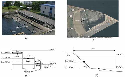
One of the survey sites was Shiosai Nagisa, which was constructed as a hybrid-type infrastructure demonstration facility in February 2008 (Furukawa 2013). It has terrace-type tidal flat structures to simulate the flat slope of a tidal flat, and multiple ground heights in a limited space in a port (Figure 2). The ground heights of the terrace at the upper, middle, and lower stages were Datum Level (D.L.) + 1.0 m, D.L. + 0.5 m, and D.L. ± 0.0 m, respectively. The monitoring stations were defined as “Shiosai Nagisa D.L. 1.0 m Sand station” (St. SN1.0S), “Shiosai Nagisa D.L. 0.5 m Sand station” (St. SN0.5S), and “Shiosai Nagisa-D.L. 0.0 m station” (St. SN0.0S). In addition, the lower part of the lower stage terrace and the circumference of the tidal flat area are surrounded by rock reefs. Access to Shiosai Nagisa is restricted to citizens, because it is located at the site of the port office.

Figure 2. Photos and monitoring stations at (a) Shiosai Nagisa and (b) Kawasaki Hama, and cross-sectional structure of (c) Shiosai Nagisa and (d) Kawasaki Hama. Photograph of (b) was downloaded from the Geospatial Information Authority of Japan (https://mapps.gsi.go.jp/)

A verification test for the construction materials of the tidal flat was conducted from July 2014 to February 2017 in Shiosai Nagisa. The middle stage of the tidal flat was divided into three compartments. The ground was excavated to approximately 0.3 m, and construction materials for the test were laid.

It was previously reported that natural sand, dredged sediment and industrial by-products should be used as construction materials for artificial habitats (Hosokawa, Hara, and Nozu 2019; Kim et al. 2014). In this study, granulated coal ash (GCA) and ferronickel slag (FNS), which are expected to have environmental benefits, were used as test construction materials. GCA was laid at the “Shiosai Nagisa D.L. 0.5 m GCA station” (St. SN0.5 G), and FNS was laid at the “Shiosai Nagisa D.L. 0.5 m FNS station” (St. SN0.5 F).

GCA is a material obtained by granulating and solidifying coal ash from thermal power plant, with a particle size of approximately 5–40 mm. GCA is porous, with a specific gravity of 2.0 g/cm³. GCA contains approximately 10% calcium oxide and magnesium oxide. The elution of GCA supplies calcium oxide and magnesium oxide to pore water, which has been reported to have environmental improvement effects such as apatitization of phosphate and adsorption and oxidation of hydrogen sulfide (Asaoka et al. 2012; Asaoka and Yamamoto 2010). FNS is a slag generated during the refining process of ferronickel, with a particle size ranging from 0.01 mm to 1 mm. FNS has a specific gravity of 3.0 g/cm³ (Kawamura et al. 2016), and contains approximately 30% calcium oxide and magnesium oxide. Further, the iron content is approximately 8%.

Another survey site is the Kawasaki Hama. Kawasaki Hama is a disaster prevention base located at the eastern end of Higashi-Ogishima, which is an artificial island. Sand beaches were constructed as disaster prevention infrastructure facilities, so that emergency supplies to urban areas can be transported using small vessels for movement through shallow waters. Kawasaki Hama was constructed in January 2008. The beach has a steep slope of 1:30, and the offshore of the beach has a subtidal zone with a slope of 1:100. The monitoring stations were defined as Kawasaki Hama D.L. 0.5 m Sand station (St. KH0.5S) and Kawasaki Hama D.L. 0.0 m Sand station (St. KH0.5S). Kawasaki Hama is usually open to citizens, and people visit this site for clam digging during spring. However, citizens are prohibited from bathing in the area during summer.

1.2. Quantification of ecosystem functions

There are four categories of ecosystem services: provisioning services, regulating services, cultural services, and supporting services (Costanza et al. 2017; Kumar 2012). Ecosystem functions and their indices for artificial tidal flats were defined according to the ecosystem services cascade (Table 1). Each ecosystem function was scored from 0 to 100 points using the following equation:

(1) $F_i=\frac{X_i}{X_R}\times 100$(1)

Table 1. Definition of ecosystem functions and their indices. The reference indicates the 100-point value of ecosystem functions

Category	Service	Function	Index	Unit of index	Reference value
Provisioning	Food provision	Fisheries resource abundance	Population of manila clam (shell length >20 mm)	population/m^2	1349
Regulating	Water purification	Organic matter consumption	Chemical Oxygen Demand purification flux with benthos	g-COD/m^2/year	502
	Carbon storage	Sediment carbon accumulation	Ignition loss	%	9.3
Cultural	Tourism	Scenery	Brightness with standard soil chart	-	5
	Recreation	Walkability	Median particle diameter	mm	0.075–2
Supporting	Life cycle maintenance	Biodiversity	Species richness of benthos	number/0.186 m^2	43
	Primary production	Microalgae abundance	Sediment chlorophyll-a	μg /cm^2	78

Here, $F_i$ is the score of the ecosystem function i, $X_i$ is the value of the index representing the ecosystem function i, and $X_i$ is the reference value of the ecosystem function i.

In many cases, multiple indices can be applied to the ecosystem function index ($X_i$). For example, the life cycle maintenance of support services can set several indices, such as habitat diversity, larval abundance, and species richness. In this case, it is possible to create a function and integrate the indices. However, it is expected that when the integrated index is used, the relationship between the index and the driving factors becomes unclear, and an appropriate analysis result regarding the impact of the design factors cannot be obtained. Therefore, we decided to assign one index to each function. The ecosystem services, functions, and indices defined in this study are described below.

The fisheries resource abundance was defined as a function of food provision as a provisioning service (Table 1). Food provision depends on various social factors. Abundance of fisheries indicates high potential for food provision. Since the representative marine product in tidal flats in Japan is clams, the index of fisheries resource abundance was defined as the number of clams with shell length exceeding 20 mm, which is the size of clams that can be caught. The reference value ($X_R$) of the fisheries resource abundance index is the highest among all number of clams data employed in the survey.

Organic matter consumption was defined as a function of water purification as a regulating service (Table 1). Organic matter purification is a biological process, and the water purification service can be enabled by considering the social demand for clean water. The chemical oxygen demand (COD) consumption amount was used as the index of organic matter consumption, which is calculated from the wet weight of benthos and the production/biomass (P/B) ratio (Okada et al. 2019). The P/B ratio was set to two with the mean value of benthic organisms in the tidal flat (Schwinghamer et al. 1986).

Sediment carbon accumulation was defined as a function of carbon storage as a regulating service (Table 1). Carbon storage is obtained by adding social factors such as the social demand of stable climate to sediment organic accumulation. The index of the sediment carbon accumulation is defined as the ignition loss (IL) in the sediment, because there is a good positive correlation between IL and carbon content in the coastal bottom mud (Fourqurean et al. 2012). The reference values of both organic matter consumption and sediment carbon accumulation were set to the maximum values of all data during the survey period.

Cultural services such as tourism, recreation, daily relaxation, and environmental education are the services that are the most difficult to evaluate among the four categories of ecosystem services (Garcia Rodrigues et al. 2017; Milcu et al. 2013). Therefore, it is difficult to set indices that directly represent the state of functions related to cultural services. Thus, we considered that ecosystem functions for cultural services can be defined as the maintenance of places where people can experience cultural value. Therefore, we considered the following two functions: scenery and walkability (Table 1).

The scenery was defined as a function of tourism because good scenery is an important sightseeing criteria. The scenery was indexed based on the lightness of the color of the bottom mud based on the standardized soil color, because people prefer brighter colored sands in beaches (Cervantes and Espejel 2008; Pranzini, Simonetti, and Vitale 2010). The reference values of the scenery were set to the maximum values of all data during the survey period.

Walkability is defined as a function of recreation, because sandy beaches are one of the most attractive places for walking in coastal areas (Kline and Swallow 1998). The median particle size of the sediment was set as the index of the walkability, because sandy sediment is an important factor in sand beach maintenance (McLachlan et al. 2013). The reference value of the walkability and the range of sand (0.1 to 2 mm) was set. The maximum value of gravel (75 mm) and minimum value of silt (0.005 mm) were defined as zero. The values between the reference value (100 points) and the 0 point were complemented with the linear interpolation method.

Biodiversity was defined as a function of life cycle maintenance on supporting services. Interactions between species in ecosystems are complex. High biodiversity tends to increase ecosystem sustainability (Aarts 1999; Burton et al. 1992). Thus, biodiversity is appropriate as a function that supports the maintenance of the life cycle of species. The index of biodiversity was set as the species richness of benthic organisms. The reference values of biodiversity were set to the maximum values for all data during the survey period.

Microalgae abundance was defined as a function of the primary production on supporting services. In coastal ecosystems, benthic microalgae are often considered to be the major primary producers, and have higher productivity than pelagic phytoplankton (Charpy-Roubaud and Sournia 1990; Miller, Geider, and MacIntyre 1996). Thus, we set the abundance of benthic microalgae as a function of the primary production. The index of microalgae abundance was set as the chlorophyll-a on sediment (S-Chl-a). The reference values of microalgae abundance were set to the maximum values for all data during the survey period.

1.3. Monitoring method

We conducted a survey on the indices of ecosystem function, environmental factors, and design factors, necessary for the analysis of the driving factors of the ecosystem functions. The details of the monitoring items and methods are shown below.

The surveys for measuring the benthos and sediments were conducted from July 2014 to December 2017 at Shiosai Nagisa and Kawasaki Hama. In addition, at Shiosai Nagisa, continuous measurement of water quality was performed in the front sea “Shiosai Nagisa water quality station” (St. SNW) from July to December of each survey year. At Kawasaki Hama, the vertical profile of water quality was measured at the “Kawasaki Hama water quality station” (St. KHW) on each survey day.

Sediment up to a depth of 0.1 m was collected three times using 25 cm × 25 cm quadrats to obtain the benthos. The collected sediment samples were screened using a 1 mm sieve, and the benthos remaining in the sieve were fixed through formalin fixation. Furthermore, the species, population number, and wet weight of the benthos were measured. The shell length was also measured for the clams.

Sediments up to a depth of 10 cm were sampled, and the surface sediment color was confirmed. They were brought back to the test room, and the grain size and IL were analyzed using the Japanese Industrial Standards method (JIS A 1204 and JIS A 1226). In addition, sediments up to a depth of 1 cm were sampled from a certain area (sand and FNS stations: 21.2 cm², GCA station: 100 cm²). The amount of S-Chl-a was analyzed for these sediment samples using JIS K0400-80-10. Here, the reason why the sampling area of the GCA station was larger than that of the other stations was that the GCA contained more gravel fractions, and it was difficult to collect the required sediments from a small sampling area.

For the continuous measurement of water quality in Shiosai Nagisa, the water temperature was measured using a salinity meter, dissolved oxygen (DO) meter, and water chlorophyll fluorescence (W-Chl-F) and turbidity meter (Compact series; JFE Advantech Co.) were moored at the level of D.L. + 0.5 m at St. SNW (Figure 2). In addition, a water level meter (Mark-5; JFE Advantech Co.) was installed at +0.1 m from the bottom of the sea at St. SNW. The water quality was measured at 30-minute intervals. In Kawasaki Hama, the water temperature, salinity, DO, W-Chl-F, and turbidity were measured at a 0.5 m pitch using a water quality meter (RINKOU; JFE Advantech Co.) at St. KHW. W-Chl-F was converted from fluorescence intensity to chlorophyll concentration (μg/L) by a calibration curve using an uranine standard solution.

1.4. Analysis of driving factors for ecosystem functions

1.4.1. Analysis using a hierarchical Bayesian model

The driving factors of ecosystem functions in the artificial tidal flat were analyzed using a statistical model. A hierarchical Bayesian model that could obtain stable solutions even for complex models was applied (Ogle 2009). In the hierarchical Bayesian model, the coefficients are not estimated points such as in the maximum likelihood estimation method, but are obtained as a posteriori probability distribution using the Markov chain Monte Carlo (MCMC) method. Therefore, it is possible to flexibly model the phenomena of ecosystems with complex structures. The hierarchical Bayesian model is given by the following equations:

(2) $F_i\left[n\right]LogNormal\left({\mu }_i\left[n\right],{\sigma }_i\right)$(2)

(3) ${\mu }_i\left[n\right]=b{0}_i+\hspace{0.17em}\sum b_{k,i}Ek\left[n\right]+\hspace{0.17em}\sum b_{l,i}Dl\left[n\right]+{\gamma }_i\left[n\right].$(3)

(4) ${\gamma }_i\left[n\right]Normal\left(0,s_i\right)$(4)

Here, we assume that the score of the ecosystem functions $F_i\left[n\right]$ follows a lognormal distribution. ${\mu }_i\left[n\right]$ and ${\sigma }_i\hspace{0.17em}$are the mean and variance of the score, respectively; $b{0}_i\hspace{0.17em}$indicates the intercepts; $n{b}_{k,i}$, and $Ek\left[n\right]$ are coefficients and variables in the environmental factors, respectively; and $b_{l,i}$ and $Dl\left[n\right]$ indicate the coefficients and variables in the design factors, respectively. ${\gamma }_i$ shows a random effect and is assumed to follow a normal distribution with a mean of zero and variance $s_i$.

The prior distributions of each coefficient provided a sufficiently wide uniform distribution. We also present a sufficiently wide uniform distribution above zero for the super-parameter of the random effect. MCMC sampling was performed with 4000 iterations per run. Moreover, the first 500 iterations were considered as a burn-in period and rejected. The calculations were performed in four runs, and it was confirmed that the $\hat{R}$ of all the coefficients was less than 1.1, and the sampling converged. The analyzed time-series data might have spurious regression when data with autocorrelation or unit root are regressed (Granger 1974). Therefore, prior to performing the hierarchical Bayesian model, the Ljung–Box test (Ljung and Box 1978) confirmed that there was no significant autocorrelation in the objective variable at a 5% significance level. It was also confirmed by the augmented Dickey–Fuller test (Leybourne 1995) that each explanatory variable was not in the unit-root process at a significance level of 5%.

The hierarchical Bayesian model did not assume direct interactions between ecosystem services to simplify the analysis and interpretation of results. The interactions between ecosystem services are expressed indirectly through the driving factors in this study. However, it has been suggested that there are direct interactions between ecosystem services (Bennett, Peterson, and Gordon 2009). Thus, the results of this study include uncertainty. We recognize that an analysis that incorporate direct relationships among ecosystem services is an open problem

The driving factors of the ecosystem functions in artificial tidal flats were considered by dividing them into environmental factors such as surrounding water quality and design factors such as the slope of tidal flats. Then, these factors were set as explanatory variables. Water temperature, salinity, DO, and W-Chl-F in seawater were used as environmental factors. Water temperature and salinity are environmental factors that represent seasonal variations and the effects of precipitation and river water. DO is an environmental factor that represents the degradation of marine organisms and ecosystems. W-Chl-F is an environmental factor that represents eutrophic conditions in the surrounding sea area. The water quality was continuously measured at Shiosai Nagisa. However, at Kawasaki Hama, only one measurement was performed at the time of the survey. Thus, there is a large difference in the frequency of measurement of water quality data. Therefore, to match the frequency of water quality measurement in the two artificial tidal flats, the water quality data of Shiosai Nagisa obtained on the same date and at the same time as the Kawasaki Hama data were used.

The designed factors were defined as the ground height, slope, and construction material, which have been reported to have a major impact on the ecosystem of tidal flats (Lee et al. 1998; Bakker and Piersma 2006). Here, the type of construction material was considered to be a categorical variable, which was attributed to a value of zero for the sand and one for GCA or FNS. In addition, the driving factors related to management were also considered as design factors. The number of years since construction was set as a design factor, because the state of the development of ecosystems or environmental conditions might fluctuate over time (Kuwae 2005). Further, utilization by citizens was used as a categorical variable to confirm the influence of utilization by people, such as clam digging in Kawasaki Hama. All variables except the categorical variables were standardized, and the standardized partial regression coefficients for each explanatory variable were obtained. Although the grain size of the sediment is also a driving factor that has a significant impact on the ecosystem in tidal flats (McLachlan 1996), it was excluded from the explanatory variables, because it is used as an index of walkability. The effect of the grain size of the basement on the ecosystem function is detected by the basement material, which is an explanatory variable.

In multiple regression analyses, higher correlation coefficients between explanatory variables lead to multicollinearity, resulting in difficulty in accurately estimating the coefficients (Zuur, Ieno, and Elphick 2010). Therefore, the correlation coefficient and variance inflation factor (VIF) between explanatory variables were calculated to confirm the presence or absence of multicollinearity, and it was confirmed that VIF was less than 10. R (version 3.5.1) and Stan (version 4.0) were used for the above analysis.

1.4.2. Path analysis

To understand the tradeoff and synergy among ecosystem functions through driving factors, the analytical results from the hierarchical Bayesian model were visualized as a path diagram. In the path diagram, the relationship between seven ecosystem functions and ten driving factors was expressed by connecting them with arrows. The driving factors that do not include zero in the 95% credible interval of the coefficient were considered to be strong paths depicted in the path diagram. The driving factors that include zero in the 95% credible interval of the coefficient were not depicted. Further, since the paths become significantly complicated by expressing seven ecosystem functions simultaneously, visualization was conducted so that the relationship between each ecosystem function and the driving factors can be easily understood.

2. Result

2.1. Monitoring data

The annual mean water temperatures of both Shiosai Nagisa and Kawasaki Hama were determined to be approximately 20°C (Table 2). The annual mean salinity values of Shiosai Nagisa and Kawasaki Hama were almost identical (20 psu), but the minimum values were different, that is, 6.5 psu at Shiosai Nagisa and 23.5 psu at Kawasaki Hama. Shiosai Nagisa is prominently affected by freshwater because there are small rivers and sewage treatment plants in the vicinity. However, the effect of freshwater on Kawasaki Hama is not prominent despite the inflow from a large river (Tama River) nearby, owing its obstructive structure. The annual mean values of DO and W-Chl-F at Shiosai Nagisa and Kawasaki Hama were almost the same. However, the variance values of DO and W-Chl-F were larger at Shiosai Nagisa. This is because continuous measurements were performed at Shiosai Nagisa, and variations in DO and W-Chl-F during the daytime and nighttime were detected in Shiosai Nagisa.

Table 2. Mean value of the water quality at Shiosai Nagisa (SN) and Kawasaki Hama (KH) during survey period (FY 2014 to FY 2017). The value in parentheses indicates the minimum value – maximum value

Site	W. Temperature (°C)	Salinity (psu)	DO (mg/L)	Chl-F (μg/L)
SN	19.8 (6.4–33.6)	27.5 (6.5–35.8)	7.8 (0.1–22.0)	5.9 (0.1–98.2)
HK	21.8 (13.2–30.0)	28.6 (23.5–31.5)	7.6 (5.3–12.3)	5.6 (0.5–31.0)

Figure 3 shows the data for (FY 2014) as a representative of the results of the continuous measurement of water quality at Shiosai Nagisa. The maximum water temperature was in August, and the minimum was in February. A rapid decrease in salinity was observed in October when a typhoon occurred. While considering the DO and W-Chl-F, it was observed that the diurnal fluctuation was large from July to October. Moreover, the values increased during the day owing to active photosynthesis. During the night, DO decreased sharply, and hypoxia, which is defined as DO below 2 mg/L, was confirmed for multiple days. From November to February, the W-Chl-F decreased to a few micrograms per liter, and the DO rose to approximately 10 mg/L.

Figure 3. Continuous measurement data of water qualities at St. SNW in (FY 2014): (a) Water temperature, (b) Salinity, (c) Dissolved oxygen, and (d) Chlorophyll Fluorescence

The grain size at Shiosai Nagisa indicated predominantly sand content (0.1 to 2 mm), except for St. SN0.5 G, where the construction material was GCA (Table 3). In St. SN0.5 G, the grain size indicated the presence of gravel (–2-to 75 mm) and was approximately 90% of the sediment. Further, the IL values at St. SN0.5 G (annual mean: 6.8%) and St. SN0.5 F (annual mean: 2.6%) were higher than those at the other sand stations. The annual mean of the lightness of the sediment was 2.3 at St. SN0.5 F and approximately 3.0 at other stations. The sediment quality at Kawasaki Hama was similar to that of the sand station at Shiosai Nagisa.

Table 3. Mean value of the sediment quality at Shiosai Nagisa (SN) and Kawasaki Hama (HK) during survey period (FY 2014 to FY 2017). The value in parentheses indicates the minimum value – maximum value

Site	Station	Grain size (%)			Ignition loss (%)	Sediment brightness
		Gravel (2–75 mm)	Sand (0.075–2 mm)	silt/clay (< 0.075 mm)
SN	SN1.0S	1.6 (0.0–11.0)	98.8 (81.0–98.0)	2.7 (1.0–8.0)	1.3 (1.0–1.4)	2.7 (2–4)
	SN0.5S	4.1 (0.0–19.0)	91.8 (74.0–97.0)	4.1 (2.0–10.0)	1.4 (1.1–1.7)	2.8 (2–5)
	SN0.5 F	1.4 (0.0–6.0)	92.2 (86.0–97.0)	6.4 (2.0–14.0)	2.5 (1.6–3.2)	2.3 (1.5–3)
	SN0.5 G	89.1 (70.0–99.0)	8.5 (1.0–27.0)	2.2 (0.0–4.0)	6.8 (3.6–9.3)	3.0 (2–4)
	SN0.0S	14.1 (6.0–38.0)	78.9 (66.0–69.0)	6.7 (2.0–14.0)	2.6 (1.4–4.2)	2.8 (1.5–4)
HK	HK0.5S	21.9 (4.0–33.0)	76.9 (66.0–96.0)	1.2 (0.0–2.0)	1.1 (0.8–1.3)	3.0 (2–5)
	HK0.0S	25.9 (2.0–49.0)	68.4 (41.0–97.0)	5.7 (1.0–20.0)	1.7 (1.1–3.4)	2.5 (2–3)

Benthic organisms such as occupied mollusks, including Ruditapes philippinarum, Musculista senhousia, and Crassostrea gigas were present at both Shiosai Nagisa and Kawasaki Hama (Figure 4). The biodiversity and wet weight of benthos tended to be low at sites with higher ground heights. The temporal variations in biodiversity of benthic organisms were small during the survey period. The seasonal variations in the wet weight of benthos were not clear; however, the annual level variances were large. The amount of S-Chl-a at Shiosai Nagisa tended to be higher than that at Kawasaki Hama. In addition, the amounts of S-Chl-a at St. SN0.5S (sand) and St. SN0.5 F (FNS), where the verification test was conducted for construction materials, were low immediately after the start of the test . Then, it increased in FY 2015, and has remained at the same level since then. Conversely, when the site with GCA was used to obtain construction material (St. SN0.5 G), it was determined that the S-Chl-a was relatively high since FY 2014.

Figure 4. Temporal variations of the species richness of benthos, wet weight of benthos, and chlorophyll-a on sediments at each station in Shiosai Nagisa and Kawasaki Hama

2.2. Quantitative valuation of ecosystem functions

Figure 5 shows the annual mean scores of the ecosystem functions evaluated using the definitions in Table 1 for each fiscal year at Shiosai Nagisa and Kawasaki Hama. The charts pertaining to the sand sites at Shiosai Nagisa (St. SN1.0S, St. SN0.5S, St. SN0.0S) show a rhombic distribution with high scores of nearly 100 points for walkability, and low scores of less than 20 points for fisheries resource abundance. The microalgae abundance, biodiversity, organic matter consumption, and sediment carbon accumulation tended to have low scores at the high ground sites at both Shiosai Nagisa and Kawasaki Hama.

Figure 5. Annual mean scores of ecosystem functions at each station in Shiosai Nagisa and Kawasaki Hama. Each Ecosystem function were evaluated using define in Table 1. The names of some ecosystem functions are abbreviations as below, Fisheries: Fisheries resource abundance, Organic matter: Organic matter consumption, Carbon: Sediment carbon accumulation and Microalgae: Microalgae abundance

At the site where the FNS was laid (St. SN0.5 F), the ecosystem function chart was similar to that of the sand site (St. SN0.5S), except for the scenery. The scenery tended to have a relatively lower value when compared to the sand site at St. SN0.5 F. Conversely, at the site where the GCA was laid (St. SN0.5 G), the walkability was relatively lower than that at St. SN0.5S, and the carbon storage and biodiversity were relatively higher.

At sites with a ground height of 0.5 m at Kawasaki Hama (St. KH0.5S), the walkability and scenery had higher values than those at Shiosai Nagisa (St. SN0.5S). However, the scores of the other functions were relatively low. Conversely, at the site with a ground height of 0.0 m at Kawasaki Hama (St. KH0.0S), the ecosystem function chart was similar to that of the site with the same ground height at Shiosai Nagisa (St. SN0.0S).

2.3. Results of analysis using the hierarchical Bayesian model

The mean values of the coefficients estimated by the hierarchical Bayesian model and the 95% credible interval are listed in Table 4. The credible interval of the Bayesian model indicates the range of values that the estimated coefficients can take at a specific percentage. Therefore, if the 95% credible interval does not straddle zero, the effect of the coefficient is certain within the 95% probability.

Table 4. Estimated coefficients of each ecosystem function model using the hierarchical Bayesian model. The value in parentheses indicates the 95% credible interval. The values in bold font indicates the coefficient that does not include zero in the 95% credible interval

	Fisheries resource abundance	Organic matter consumption	Sediment carbon accumulation	Scenery	Walkability	Biodiversity	Microalgae abundance
Intercept	−0.59 (−2.61–1.42)	1.54 (1.06–2.03)	2.91 (2.82–3.00)	4.02 (3.93–4.12)	4.60 (4.59–4.61)	3.54 (3.40–3.68)	2.26 (1.85–2.67)
Temperature	−2.32 (−4.70–0.11)	−0.75 (−1.35 – −0.18)	−0.03 (−0.13–0.08)	−0.03 (−0.14–0.08)	0.00 (−0.02–0.01)	−0.37 (−0.54 – −0.20)	0.58 (0.10–1.07)
Salinity	0.64 (−2.08–0.78)	−0.01 (−0.35–0.34)	−0.04 (−0.10–0.02)	−0.01 (−0.07–0.06)	0.00 (−0.01–0.00)	−0.06 (−0.16–0.04)	0.17 (−0.12–0.45)
DO	−1.20 (−3.06–0.70)	−0.51 (−0.96 – −0.06)	−0.02 (−0.11–0.06)	0.01 (−0.08–0.09)	−0.01 (−0.02–0.00)	−0.16 (−0.29–0.00)	0.32 (−0.06–0.69)
W-Chl-F	2.21 (0.22–4.13)	0.62 (0.15–1.09)	0.02 (−0.06–0.11)	−0.02 (−011 – 0.07)	0.00 (−0.01–0.01)	0.23 (0.10–0.37)	−0.29 (−0.69–0.10)
Ground height	−1.53 (−2.89 – −0.19)	−0.71 (−1.03 – −0.38)	−0.22 (−0.27 – −0.16)	−0.01 (−0.07–0.05)	0.00 (−0.01–0.01)	−0.27 (−0.36 – −0.17)	0.19 (−0.46–0.08)
Slope	−1.57 (−3.44–0.35)	−0.70 (−1.03 – −0.38)	0.00 (−0.08 – −0.08)	0.12 (0.04–0.21)	0.00 (−0.01–0.01)	−0.38 (−0.51 – −0.26)	−0.59 (−0.95 – −0.22)
Material (FNS:Sand)	−1.39 (−5.38–2.57)	−0.82 (−1.86–0.23)	0.39 (0.21–0.57)	−0.21 (−0.40 – −0.02)	0.01 (−0.02–0.03)	0.19 (−0.10–0.50)	0.77 (−0.06–1.61)
Material (GCA:Sand)	−3.50 (−7.63–0.61)	−0.65 (−1.67–0.36)	1.39 (1.22–1.57)	0.05 (−0.13–0.23)	−0.25 (−0.27 – −0.23)	0.33 (0.02–0.61)	1.74 (0.88–2.55)
Elapsed time	−1.38 (−3.22–0.50)	−1.03 (−1.50 – −0.56)	0.00 (−0.08–0.09)	−0.05 (−0.13–0.04)	0.00 (−0.01–0.01)	0.01 (−0.12–0.15)	0.92 (0.52–1.31)
Citizen use	−1.24 (−6.11–3.82)	−0.59 (−1.71–0.58)	−0.37 (−0.58 – −0.16)	−0.08 (−0.30–0.12)	0.00 (−0.02–0.03)	−0.05 (−0.39–0.29)	−2.05 (−3.03 – −1.14)

In the fisheries resource abundance, the explanatory variables in which the 95% credible interval does not include zero were W-Chl-F for environmental factors and ground height for design factors. However, the ground height had a negative coefficient; that is, it was observed that as the ground height increased, the fisheries resource abundance decreased. This result is valid because the abundance of benthic animals on tidal flats decreases as the ground height increases (Kuwae 2005). W-Chl-F had a positive value, which is a reasonable result that when the food (W-Chl-F) in seawater is massive, the fisheries resource is increased.

In organic matter consumption, the explanatory variables for which the 95% credible interval does not include zero were the water temperature, DO, and W-Chl-F for environmental factors and the ground height, slope, and elapsed time for design factors. The coefficients of water temperature, DO, ground height, and slope were negative. The W-Chl-F coefficient had a positive value. These results are reasonable from the perspective of coastal ecology, except DO. High temperatures result in a reductive environment in sediment due to the high activity of microorganisms. As a result, the benthic organism mass is reduced. The results of W-Chl-F can be explained in the same way as the fishery resources abundance. In addition, the results of ground height and slope are consistent with those of previous studies (Lee et al. 1998; Kuwae, 2005). It is difficult to judge the validity of the elapsed time coefficient, but it can be said that the result is opposite to the concept of the autonomous development process of the ecosystems in artificial habitat that was proposed by (Kuwae 2005).

In the sediment carbon accumulation, the explanatory variables for which the 95% credible interval does not include zero were not environmental factors. Conversely, while considering the design factors, the ground height, construction material FNS and GCA, and citizen use were explanatory variables with 95% confidence intervals that did not include zero. The coefficients of ground height and citizen use had a negative value. These results are reasonable, because both high ground height and clamming by citizens tend to reduce biomass and carbon accumulation. In addition, the coefficients of the construction material FNS and GCA were positive, indicating that FNS and GCA had a higher carbon content than sand. This is a property of the materials, rather than the ecosystem functions. The carbon stock of FNS and GCA in the manufacturing process should be regarded as carbon storage from the perspective of life cycle assessment, rather than an ecosystem function. In this study, we could not separate the carbon stock in the manufacturing process from the carbon accumulation in the ecosystem function; therefore, the analysis of the effects of FNS and GCA on carbon storage function is excluded from subsequent discussions.

In the scenery, explanatory variables for which the 95% credible intervals did not include zero were not considered environmental factors. Conversely, in the design factors, the slope and construction material (FNS) were explanatory variables that did not include zero in the 95% credible interval. The coefficient of the slope was positive. Therefore, as the slope became steeper, the scenery tended to increase. This result is reasonable, because the steeper slope reduces the biomass of benthic animals and organic matter accumulation (Lee et al. 1998). The coefficient of the construction material FNS was negative because the FNS color itself was dark.

In walkability, only the construction material GCA was an explanatory variable that did not include zero in the 95% credible interval. The coefficient of the construction material GCA was a negative value, indicating that GCA has a lower walkability when compared to sand because of the original GCA granularity.

In biodiversity, the explanatory variables for which the 95% credible interval does not include zero were water temperature and W-Chl-F for environmental factors and ground height, slope, and construction material GCA for design factors. The coefficient of W-Chl-F was positive, implying that as the amount of food increased, the biodiversity increased. Conversely, the coefficient of water temperature was negative, implying that high temperature reduces biodiversity due to reductive conditions. The coefficients of ground height and slope were negative. The coefficients of GCA were positive. These design factor results are consistent with those of previous studies (Lee et al. 1998; Kuwae, 2005; Kim et al. 2014).

In the microalgae abundance function, the explanatory variables for the 95% credible interval that does not include zero were not environmental factors. Conversely, while considering the design factors, slope, construction material GCA, and elapsed time were variables that did not include zero in the 95% credible interval. These results are consistent with those of previous studies (Lee et al. 1998; Nakamoto et al. 2015). The coefficient of the slope was negative. The coefficient of the construction material GCA was positive. The coefficient of the elapsed time was also positive, indicating that as more time elapsed after the construction, and the microalgae abundance function increased.

2.4. Results of path analysis

Figure 6 shows the visualized path diagram. The environmental and design factors are shown on the left and right sides, respectively, of Figure 6. In addition, the functions related to provisioning, regulating, cultural, and supporting services are arranged on the upper, left, lower, and right sides, respectively, of the circle. The relationship between driving factors and ecosystem functions that do not include zero in the 95% credible interval is indicated by arrows. At the start of the arrow, the positive and negative directions of the coefficients are described, and on the line, the values of the coefficients are described. Additionally, arrows of the FNS and GCA to carbon storage were excluded because the carbon storage of FNS and GCA includes not only ecosystem functions but also manufacturing processes. The results in Figure 6 were obtained from the data of this study. Therefore, it should be noted that generalization to cases in which the survey period or environment conditions are significantly different from this study is desired.

Figure 6. Visualized path analysis of the driving factors of ecosystem functions. The relationship between driving factors and ecosystem functions that do not include zero in the 95% credible interval is indicated by arrows. At the start of the arrow, the positive and negative directions of the coefficients are described, and on the line, the values of the coefficients are described. The arrows of the FNS and GCA to carbon storage are excluded because the carbon storage of FNS and GCA includes not only ecosystem functions but also manufacturing processes

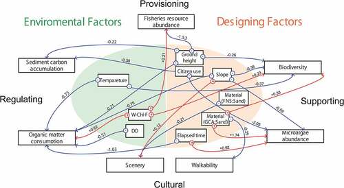
2.4.1. Environmental factors

The water temperature demonstrated a negative correlation to organic matter consumption and biodiversity, and a high water temperature had the effect of weakening these two functions. W-Chl-F demonstrated the effect of enhancing fisheries resource abundance, organic matter consumption, and biodiversity. Furthermore, DO weakened organic matter consumption.

2.4.2. Design factors

The ground height was negatively correlated with fisheries resource abundance, organic matter consumption, sediment carbon accumulation, and biodiversity. High ground heights had the effect of weakening these four functions. The slope demonstrated a negative correlation with organic matter consumption, biodiversity, and microalgae abundance, and demonstrated a positive correlation with scenery.

The utilization of FNS as the construction material was negatively correlated with the scenery; the use of FNS reduced the scenery functions. Conversely, the use of GCA as the construction material demonstrated a positive correlation with the biodiversity and microalgae abundance, and it had a negative correlation with walkability. The use of GCA enhanced the functions of biodiversity and microalgae abundance while reducing the function of walkability.

The elapsed time demonstrated a positive correlation with the microalgae abundance and a negative correlation with organic matter consumption. The factor of citizen use had a negative correlation with sediment carbon accumulation and microalgae abundance. Therefore, these two functions might deteriorate when the artificial tidal flat is opened to citizens.

3. Discussion

3.1. Scores for ecosystem functions

Shiosai Nagisa and Kawasaki Hama are green port structures that construct small tidal flats while maintaining or supplementing the function of a port. The structures of Shiosai Nagisa and Kawasaki Hama are significantly different. Shiosai Nagisa has a terrace-type structure, whereas the beach of Kawasaki Hama has a beach-type structure (Figure 2). Despite these structural differences, the differences in annual mean scores for ecosystem functions between Shiosai Nagisa with sand (St. SN1.0S, St. SN0.5S, St. SN0.0S) and Kawasaki Hama (St. KH0.5S, KH0.0S) were not clear (Figure 5). This suggests that laying a sand base in the intertidal zone regardless of the structure can yield similar ecosystem functions. The slight difference between Shiosai Nagisa and Kawasaki Hama is thought to be derived from specific driving factors such as slope or W-Chl-F. Conversely, the annual mean scores at the GCA-covered site (St. SN0.5 G) showed specific charts that differed from those at other sites. This suggests that different ecosystem functions can be obtained by changing the construction material even under the same environmental conditions. In addition, the annual mean score of ecosystem functions showed annual fluctuations. Thus, it is considered that ecosystem functions vary according to driving factors such as annual weather factors, and changes in ecosystems over time. We discuss the driving factors of ecosystem functions from the statistical models and path analysis results in the following section. In addition, this paper discusses aspects requiring attention while designing artificial tidal flats based on ecosystem functions.

It should be noted that the scores for ecosystem functions are indicated by the ratio to the reference values, and differences in scores between ecosystem functions do not imply superiority or inferiority between ecosystem functions. The fisheries resource abundance and organic matter consumption with a low annual mean score imply a large fluctuation in each survey day and at all sites. The scenery and walkability with a high annual mean score imply a small fluctuation in each survey day and at all sites. Thus, the difference in scores between ecosystem functions does not indicate the superiority or inferiority between ecosystem functions, but the magnitude of the variance in the indices of each ecosystem function should be considered.

3.2. Environmental factors affecting ecosystem functions

The W-Chl-F in seawater affected the maximum number of ecosystem functions in environmental factors, which demonstrated positive effects on fisheries resource abundance, organic matter consumption, and biodiversity (Figure 6). The lack of food in winter is a key factor contributing to the depletion of clams in the natural tidal flats in Tokyo Bay, which has been reported since the 1990s (Kakino, Kazuya, and Hsegawa 1995). Model analysis showed that winter feeding shortage is a key growth-inhibiting factor in Shiosai Nagisa (Kawamura et al. 2016). Since W-Chl-F in Shiosai Nagisa was very low in winter (Figure 2), food for benthos might be scarce, which results in reduced fisheries resource abundance, organic matter consumption, and biodiversity. In other inner bays of Japan, it was reported that oligotrophication has manifested in recent years due to the pollutant load regulation, that has continued to grow since the 1970s (Abo and Yamamoto 2019). Moreover, it was suggested that the feed quantity becomes an important environmental factor that controls the ecosystem function of tidal flats in Tokyo Bay.

It is well known that large-scale aquatic hypoxia occurs in the northern region every year in Tokyo Bay, and ecosystems have sustained significant damage (Kodama and Horiguchi 2011). However, there was no positive correlation between DO and ecosystem functions (Figure 6). Furthermore, there was a negative correlation between organic matter consumption and DO, implying that organic matter consumption increases as DO decreases (Figure 6). Suzuki et al. (1998) reported that as the oxygen levels deteriorated, the species with strong resistance to oxygen demonstrated better survivability and increased biomass in tidal flats. The dominant species in Shiosai Nagisa and Kawasaki Hama were relatively anoxic-resistant species such as clams, which may have the same tendency as described by Suzuki et al. (1998). However, the DO data in this study is the instantaneous value of the survey data, and it might not be able to detect the effect of poor oxygen levels. The clam, which is an anoxic-resistant species, is unaffected when exposed to anaerobic conditions for several days. However, glycogen content, which is used for anaerobic metabolism in the clam, decreased due to successive exposure to anaerobic conditions, and their mortality rate increased (Kozuki et al. 2013). Multiple regression analysis using the instantaneous value of DO as an explanatory variable cannot detect the time lag of the effects of such anoxia. Understanding the relationship between anoxia and ecosystem functions requires the monitoring of ecosystem functions at shorter time intervals, and the application of time-series analysis or state-space models.

The water temperature demonstrated a negative correlation with organic matter consumption and biodiversity (Figure 6). Although the data are not shown in this paper, the dissolved sulfide concentration in the pore water in the sediments in summer reaches several parts per million at Shiosai Nagisa (Mito et al. 2018). The negative relationship between the water temperature and the ecosystem function indicates that the damage to benthic organisms from sulfide increases at high temperatures.

3.3. Design factors affecting ecosystem functions

Design factors affected more ecosystem functions than environmental factors (Figure 6). The two design factors, ground height and slope, affected all ecosystem functions except walkability (Figure 6). In tidal flats, the ground height is a critical factor in determining flood duration, and as the flood duration decreases, the environment becomes more severe for organisms (Kuwae 2005). In addition, flat slopes also tend to easily deposit organic matter and floating larvae, resulting in higher bioactivity (Lee et al. 1998). Therefore, it is considered that the ground height and slope were negatively correlated with three ecosystem functions (organic matter consumption, sediment carbon accumulation, and biodiversity) indexed based on the benthic organisms. Conversely, as the slope becomes steeper, a more positive correlation with the scenery is obtained. It is considered that a steeper slope has minimal organic matter accumulation and low biomass. Consequently, a clean sandy beach can be retained.

　 Considering the type of construction material, it becomes clear that different types of materials provided different ecosystem functions when compared to natural sand (Figure 6). GCA improved the microalgae abundance. It is considered that this improved the activity of microalgae, owing to the porous structure of GCA and easy attachment of microalgae to such a structure (Nakamoto et al. 2015), as well as the supply of nutrients from GCA (Asaoka, Yamamoto, and Yamamoto 2008). GCA was also positively related to biodiversity. This is because over 90% of gravel is comprised of GCA (Table 2). Moreover, in addition to the organisms found in other tidal flats, several attached organisms such as oysters or barnacles adhere to GCA. Conversely, the gravel of GCA is a negative factor for walkability. FNS has a negative relationship with the scenery, because FNS is a black-colored material.

　 The management of artificial tidal flats after construction was also clarified to be a factor affecting ecosystem functions (Figure 6). The elapsed time after construction was positively related to the microalgae abundance, but negatively related to organic matter consumption (Figure 6). It is known that the growth of benthic microalgae on sediments, which is an index of the microalgae abundance, is closely related to the development of biofilms formed by interactions with microorganisms and the activities of benthic animals (Carpentier et al. 2013; Decho 2000). Therefore, it is considered that the positive relationship with elapsed time captures the process in which biofilms form over time, and the growth of benthic microalgae becomes active (Figure 4). In addition, the wet weight of benthos, which is an indicator of organic matter consumption, tended to be low at all sites in 2017 (Figure 4). As mentioned earlier, this may be the result of the massive death of benthic animals due to the anaerobic water mass that occurred during this period, which was not considered in this study. In fact, anaerobic water masses have been identified near Shiosai Nagisa and Kawasaki Hama from late June to early July 2017 (Kanagawa Prefecture 2020). Thus, the relationship between organic matter consumption and elapsed time might have captured the phenomenon rather than continuous time changes. It has been reported that approximately two to six years are required before the ecosystem in a developed tidal flat reaches equilibrium (Kuwae 2005). Artificial tidal flats in urban areas such as Tokyo Bay are susceptible to events such as aquatic hypoxia and blue tides, and time-series ecosystem function variations might be more complex and nonlinear.

While considering citizen use, which is another design factor in management, a negative correlation was obtained between the microalgae abundance and sediment carbon accumulation (Figure 6). Considering the microalgae abundance, an oligotrophic condition was considered to be prevalent in Kawasaki Hama, when compared to Shiosai Nagisa. This is because the nutrients are regularly removed in the form of clams, owing to the prevalence of clam digging. It is also possible that the sediment carbon accumulation was reduced by removing carbon as clams through clam digging. Furthermore, plowing of the bottom mud by clam digging occurs commonly, which might accelerate the decomposition of organic matter and result in the reduction of sediment carbon accumulation. From these trends, it is considered that opening tidal flats to citizens has the effect of lowering the nutritional state of tidal flats by removing nutrients and organic substances through clam digging. Incidentally, citizen use is expressed as a categorical variable where the case of use is set as one, and the case of no use is set as zero. Therefore, attention should be paid to the possibility that the effects of the driving factors that are not incorporated in explanatory variables are included. The use of explanatory variables that can directly express usage conditions such as usage time for citizens will enable a more accurate analysis.

3.4. Design based on ecosystem functions

When designing artificial tidal flats as a green infrastructure to supply various ecosystem services, it can be expected that further development of the analytical method of ecosystem functions shown in this study will enable a design based on the required ecosystem services. At this time, trade-offs and synergies among ecosystem services must be noted (Bennett, Peterson, and Gordon 2009; Martín-López et al. 2014; Turkelboom et al. 2018). Tradeoff and synergy among ecosystem services can be defined as two relationships: indirect relationships through common driving factors and direct relationships between ecosystem services (Bennett, Peterson, and Gordon 2009). These relationships also vary with the index and habitat used, and are highly complex (Martín-López et al. 2014). Therefore, it is important to conduct a design that can optimize ecosystem services while considering the underlying mechanisms for tradeoff and synergy between ecosystem functions.

As an example, let us consider a case of designing an artificial tidal flat that has two purposes: a beach where people can rest (scenery and walkability) and a protected area for marine organisms (biodiversity, microalgae abundance). As shown in (Figure 6), the upper tidal zones with high ground height are primarily used as beaches for people to rest, where biodiversity and microalgae abundance are low. Conversely, biodiversity and microalgae abundance increased in the lower tidal zone where ground height was low. Therefore, the maximum values of the ecosystem functions related to the two purposes can be obtained by considering an appropriate design. For example, the slope of the upper tidal zone is steepened and natural sand is laid. Further, for the lower tidal zone, a wide area with a gentle slope is installed. For the lower tidal zone to be a protected area for organisms, the application of construction materials to enhance the microalgae abundance and biodiversity such as GCA can also be considered. By applying a design based on ecosystem functions, it can also be expected that the utilization of the artificial tidal flat to be created depending on the purpose will be clarified, and spatial zoning will be facilitated.

Conversely, it is considered that the tradeoff and synergy of the ecosystem services might differ from the tradeoff and synergy analyzed based on ecosystem functions. For example, provisioning and regulating services have often been reported to demonstrate a tradeoff (Carpenter et al. 2009; Martín-López et al. 2014). However, the relationship through the driving factor between fisheries resource abundance, organic matter consumption, and sediment carbon accumulation in this study was in the same fluctuation direction rather than tradeoff. This can be attributed to the fact that ecosystem functions are potential ecosystem services that do not consider social factors. In fact, when carefully considered, the results of the analysis in this study demonstrate a trade-off between provisioning and regulating services. People use artificial tidal flats for clam digging (provisioning service), which reduces sediment carbon accumulation (regulating service) (Figure 6). Thus, in a design based on ecosystem functions, it is important to clearly recognize the differences between ecosystem functions and ecosystem services.

It should also be noted that the coefficients obtained from the statistical model of this study were estimated based on limited monitoring data. For example, the relationship between ground height and ecosystem function was obtained in the range of D.L. ± 0.0 m – D.L. + 1.0 m. Even if the ground height was designed to be deeper than D.L. ± 0.0 m to obtain the organic matter consumption more effectively, the organic matter consumption will not be obtained as expected. This is because benthic animals abundance increase in the intertidal zone and decrease in the subtidal zone (Kuwae 2005). In addition, in this study, data from only two artificial tidal flats were used. Therefore, design factors related to the overall shape of tidal flats, such as the terrace width or tidal flat area, were not analyzed. Although it is ideal to integrate all the data that can be analyzed, it is unrealistic in terms of cost and labor. Moreover, in several cases, statistical models involve uncertainties. When designing based on ecosystem functions, it is important to recognize the limitations of statistical models and design them such that the functions required in the artificial habitat can be maximized.

4. Conclusion

The aim of this study was to establish a functional design technique that can optimize the ecosystem service of artificial habitats in urban areas. The driving factors of the seven ecosystem functions were analyzed in two artificial tidal flats in Tokyo Bay. It was shown that the ecosystem functions of the artificial tidal flat in Tokyo Bay could be controlled via design factors such as ground height, slope, and construction material. It is considered that the ecosystem service can be optimized by reflecting this information in the design of the artificial tidal flat. It was also clarified that the microalgae abundance of seawater in winter is an important environmental factor. This finding will become important for the spatial arrangement of tidal flats.

Conversely, it should be noted that the habitat targeted in this study is only artificial tidal flats, and the knowledge obtained cannot be applied to other habitats. To extend the application range of our functional design, it is also necessary to study other artificial habitats. Therefore, it is important to promote research on meta-analysis, where the data of several artificial habitats are collected. In recent years, open data systems have been developed to enable such studies in Japan (Tokyo Bay Environmental Information Center 2020). The progress of these studies is awaited.

Finally, to implement the design based on ecosystem functions, it is necessary for consensus building among stakeholders based on ecosystem services. A consensus-building tool for this purpose and an assessment method that reflects the opinions of stakeholders are also being developed (Okada et al. 2019). To advance artificial habitats in urban areas, it is important to consistently evaluate ecosystem services from planning to design and management.

Acknowledgments

We are grateful to Dr. Tomohiro Kuwae of the Port and Airport Research Institute for his collaboration in the early stages of this work. We would like to thank Professor Yoshiyuki Nakamura of Yokohama National University, Associate Professor Tadashi Hihino of Hiroshima University, Chugoku Electric Power Co., Inc., and the Japan Mining Association for their advice and cooperation on verification tests for construction materials. We would like to thank Editage (www.editage.com) for English language editing.

Disclosure statement

No potential conflict of interest was reported by the author(s).

References

- Aarts, B. G. W. 1999. “Ecological Sustainability and Biodiversity.” International Journal of Sustainable Development & World Ecology 6 (2): 89–102. doi:10.1080/13504509909469998.
- Abo, K., and T. Yamamoto. 2019. “Oligotrophication and Its Measures in the Seto Inland Sea, Japan.” Bulletin of Japan Fisheries Research and Education Agency 49: 21–16.
- Ahn, C., and S. Schmidt. 2019. “Designing Wetlands as an Essential Infrastructural Element for Urban Development in the Era of Climate Change.” Sustainability 11 (7): 1920. doi:10.3390/su11071920.
- Albert, C., J. H. Spangenberg, and B. Schröter. 2017. “Nature-Based Solutions: Criteria.” Nature 543 (7645): 315. doi:10.1038/543315b.
- Asaoka, S., S. Hayakawa, K. Kim, K. Takeda, M. Katayama, and T. Yamamoto. 2012. “Combined Adsorption and Oxidation Mechanisms of Hydrogen Sulfide on Granulated Coal Ash.” Journal of Colloid and Interface Science 377 (1): 284–290. doi:10.1016/j.jcis.2012.03.023.
- Asaoka, S., and T. Yamamoto. 2010. “Characteristics of Phosphate Adsorption onto Granulated Coal Ash in Seawater.” Marine Pollution Bulletin 60 (8): 1188–1192. doi:10.1016/j.marpolbul.2010.03.032.
- Asaoka, S., T. Yamamoto, and K. Yamamoto. 2008. “A Preliminary of Coastal Sediment Amendment with Granurated Coal Ash Nutrient Elution Test and Experiment on Skeltonema Costatumu Growth.” Journal of Japan Society on Water Environment 31: 456–462. in Japanese.
- Bakker, J. P., and T. Piersma. 2006. “Restoration of Intertidal Flats and Tidal Salt Marshes.” In Restoration Ecology: The New Frontier, edited by J. V. Andel and J. Aronson. 174-192. USA: Blackwell Publishing.
- Barbier, E. B., S. D. Hacker, C. Kennedy, E. W. Koch, A. C. Stier, and B. R. Silliman. 2011. “The Value of Estuarine and Coastal Ecosystem Services.” Ecological Monographs 81 (2): 169–193. doi:10.1890/10-1510.1.
- Bennett, E. M., G. D. Peterson, and L. J. Gordon. 2009. “Understanding Relationships among Multiple Ecosystem Services.” Ecology Letters 12 (12): 1394–1404. doi:10.1111/j.1461-0248.2009.01387.x.
- Burton, P.J., Balisky, A.C., Coward, L.P., Cumming, S.G. and D. D. Kneeshaw. 1992. “The value of managing for biodiversity.” The Forestry Chronicle 68, 225–237. doi:10.5558/tfc68225-2
- Carpenter, S. R., H. A. Mooney, J. Agard, D. Capistrano, R. S. Defries, S. Díaz, T. Dietz et al. 2009. “Science for Managing Ecosystem Services: Beyond the Millennium Ecosystem Assessment.” Proceedings of the National Academy of Sciences of the United States of America 106 (5): 1305–1312. DOI:10.1073/pnas.0808772106.
- Carpentier, A., S. Como, C. Dupuy, C. Lefrançois, A. Carpentier, S. Como, C. Dupuy, C. Lefrançois, and E. F. Feed. 2013. “Feeding Ecology of Liza Spp. In a Tidal Flat: Evidence of the Importance of Primary Production (Biofilm) and Associated Meiofauna.” Journal of Sea Research 92: 86–91. doi:10.1016/j.seares.2013.10.007.
- Cervantes, O., and I. Espejel. 2008. “Design of an Integrated Evaluation Index for Recreational Beaches.” Ocean & Coastal Management 51 (5): 410–419. doi:10.1016/j.ocecoaman.2008.01.007.
- Charpy-Roubaud, C., and A. Sournia. 1990. “The Comparative Estimation of Phytoplanktonic, Microphytobenthic and Macrophytobenthic Primary Production in the Oceans.” Marine Microbial Food Webs 4: 31–57.
- Cohen-Shacham, E., G. Walters, C. Janzen, and S. Maginnis. 2016. “Nature-Based Solutions to Address Global Societal Challenges.” Switzerland: IUCN. doi:10.2305/IUCN.CH.2016.13.en.
- Costanza, R., R. de Groot, L. Braat, I. Kubiszewski, L. Fioramonti, P. Sutton, S. Farber, and M. Grasso. 2017. “Twenty Years of Ecosystem Services: How Far Have We Come and How Far Do We Still Need to Go?” Ecosystem Services 28: 1–16. doi:10.1016/j.ecoser.2017.09.008.
- de Groot, R., L. Brander, S. van der Ploeg, R. Costanza, F. Bernard, L. Braat, M. Christie, et al. 2012. “Global Estimates of the Value of Ecosystems and Their Services in Monetary Units.” Ecosystem Services 1 (1): 50–61. doi:10.1016/j.ecoser.2012.07.005.
- de Groot, R. S., R. Alkemade, L. Braat, L. Hein, and L. Willemen. 2010. “Challenges in Integrating the Concept of Ecosystem Services and Values in Landscape Planning, Management and Decision Making.” Ecological Complexity 7 (3): 260–272. doi:10.1016/j.ecocom.2009.10.006.
- Decho, A. W. 2000. “Microbial Biofilms in Intertidal Systems: An Overview.” Continental Shelf Research 20 (10–11): 1257–1273. doi:10.1016/S0278-4343(00)00022-4.
- Elliott, M., D. Burdon, K. L. Hemingway, and S. E. Apitz. 2007. “Estuarine, Coastal and Marine Ecosystem Restoration: Confusing Management and Science – A Revision of Concepts.” Estuarine, Coastal and Shelf Science 74 (3): 349–366. doi:10.1016/j.ecss.2007.05.034.
- Elmqvist, T., H. Setälä, S. N. Handel, S. van der Ploeg, J. Aronson, J. N. Blignaut, E. Gómez-Baggethun, D. J. Nowak, J. Kronenberg, and R. de Groot. 2015. “Benefits of Restoring Ecosystem Services in Urban Areas.” Current Opinion in Environmental Sustainability 14: 101–108. doi:10.1016/j.cosust.2015.05.001.
- Fourqurean, J. W., C. M. Duarte, H. Kennedy, N. Marbà, M. Holmer, M. A. Mateo, E. T. Apostolaki, et al. 2012. “Seagrass Ecosystems as a Globally Significant Carbon Stock.” Nature Geoscience 5 (7): 505–509. doi:10.1038/ngeo1477.
- Furukawa, K., and T. Okada. 2006. “Tokyo Bay: Its Environmental Status - Past, Present and Future.” In The Environment in Asia Pacific Harbors, edited by E. Wolanski, 15–34, Dordrecht: Springer.
- Furukawa, K. 2013. “Case Studies for Urban Wetlands Restoration and Management in Japan.” Ocean & Coastal Management 81: 97–102. doi:10.1016/j.ocecoaman.2012.07.012.
- Furukawa, K., M. Atsumi, and T. Okada. 2019. “Importance of Citizen Science Application for Integrated Coastal Management - Change of Gobies’ Survival Strategies in Tokyo Bay, Japan.” Estuarine, Coastal and Shelf Science 228: 106388. doi:10.1016/j.ecss.2019.106388.
- Garcia Rodrigues, J., A. Conides, S. Rivero Rodriguez, S. Raicevich, P. Pita, K. Kleisner, C. Pita, et al. 2017. “Marine and Coastal Cultural Ecosystem Services: Knowledge Gaps and Research Priorities.” One Ecosystem 2 :e12290. doi:10.3897/oneeco.2.e12290.
- Granger, C. W. J. and P. Newbold. 1974. “Spurious Regressions in Econometrics.” Journal of econometrics 2 (2), 111–120. doi:10.1016/0304-4076(74)90034-7
- Guerry, A. D., M. H. Ruckelshaus, K. K. Arkema, J. R. Bernhardt, G. Guannel, C. K. Kim, M. Marsik, et al. 2012. “Modeling Benefits from Nature: Using Ecosystem Services to Inform Coastal and Marine Spatial Planning.” International Journal of Biodiversity Science, Ecosystem Services and Management 8 (1–2): 107–121. doi:10.1080/21513732.2011.647835.
- Hosokawa, S., T. Hara, and M. Nozu. 2019. “Advanced Engineering Techniques and Environmental Measures for Beneficial Sediment Use in Japan.” Hobart: Australasian Coasts and Ports 2019 Conference, 611–616.
- Kakino, J., H. Kazuya, and K. Hsegawa. 1995. “‘Winter Life and Mortality in Japanese Littleneck Clam Ruditapes Phillippinarum on the Banzu Tidal Flat, Tokyo Bay.’ Fish.” Engineering 32: 23–32. in Japanese.
- Kanagawa Prefecture. 2020. “Tokyo Bay Dissolver Oxygen Information” http://www.pref.kanagawa.jp/docs/mx7/cnt/f430693/p550034.html.2020.09.10 (in Japanese).
- Kawamura, K., Y. Akakura, T. Haruta, Y. Mito, T. Ssugano, K. Kurisu, K. Hino, Y. Nakamura, T. Hibino, and T. Okada. 2016. “Applying Recycled Resources to a Pro-Environmental Seawall and Its Characteristics as a Habitat for Manila Clams.” Journal of Japan Society of Civil Engineers, Series B2 (Coastal Engineering) 72 (I): 1405–I_1410. doi:10.2208/kaigan.72.I_1405.
- Kim, K., T. Hibino, T. Yamamoto, S. Hayakawa, Y. Mito, K. Nakamoto, and I. Lee. 2014. “Field Experiments on Remediation of Coastal Sediments Using Granulated Coal Ash.” Marine Pollution Bulletin 83 (1): 132–137. doi:10.1016/j.marpolbul.2014.04.008.
- Kline, J. D., and S. K. Swallow. 1998. “The Demand for Local Access to Coastal Recreation in Southern New England.” Coastal Management 26 (3): 177–190. doi:10.1080/08920759809362351.
- Kodama, K., and T. Horiguchi. 2011. “Effects of Hypoxia on Benthic Organisms in Tokyo Bay, Japan: A Review.” Marine Pollution Bulletin 63 (5–12): 215–220. doi:10.1016/j.marpolbul.2011.04.022.
- Kozuki, Y., R. Yamanaka, M. Matsushige, A. Saitoh, S. Otani, and T. Ishida. 2013. “The after-Effects of Hypoxia Exposure on the Clam Ruditapes Philippinarum in Omaehama Beach, Japan.” Estuarine, Coastal and Shelf Science 116: 50–56. doi:10.1016/j.ecss.2012.08.026. in Japanese.
- Kumar, P. 2012. “The Economics of Ecosystems and Biodiversity: Ecological and Economic Foundations.” Econ Ecosyst Biodivers Ecol Econ Found 1–411. doi:10.4324/9781849775489.
- Kuwae, T. 2005. “Development and Self-Stabilization of Restored and Created Intertidal Flat Ecosystems.” Journal of Japan Society of Civil Engineers 790: 25–34. in Japanese.
- La Notte, A., D. D’Amato, H. Mäkinen, M. L. Paracchini, C. Liquete, B. Egoh, D. Geneletti, and N. D. Crossman. 2017. “Ecosystem Services Classification: A Systems Ecology Perspective of the Cascade Framework.” Ecological Indicators 74: 392–402. doi:10.1016/j.ecolind.2016.11.030.
- Lee, J. G., W. Nishijima, T. Mukai, K. Takimoto, T. Seiki, K. Hiraoka, and M. Okada. 1998. “Factors to Determine the Functions and Structures in Natural and Constructed Tidal Flats.” Water Research 32 (9): 2601–2606. doi:10.1016/S0043-1354(98)00013-X.
- Leybourne, S. J. 1995. “Testing for Unit Roots Using Forward and Reverse Dickey-Fuller Regressions.” Department of Economics, University of Oxford 57 (4): 559–571. doi:10.1111/j.1468-0084.1995.tb00040.x
- Ljung, G. M., and G. E. P. Box. 1978. “On a Measure of Lack of Fit in Time Series Models.” Biometrika 65 (2): 297–303. doi:10.1093/biomet/65.2.297.
- López-Portillo, J., R. R. Lewis Ш, P. Saenger, A. Rovai, N. Koedam, F. Dahdouh-Guebas, C. Agraz-Hemandez, and V. H. Rivera-Monroy. 2017. “Mangrove Forest Restoration and Rehabilitation.” In Mangrove Ecosystems: A Global Biogeographic Perspective, edited by R. R. Ewis III, Saenger, P. Rovai, A. Koedam, F. Dahdouh-Guebas, V. H. Rivera-Monroy, S. Y. Lee, E. Kristensen, and R. Twilley, 301-345. Cham: Springer. doi:10.1007/978-3-319-62206-4_10.
- Luederitz, C., E. Brink, F. Gralla, V. Hermelingmeier, M. Meyer, L. Niven, L. Panzer, et al. 2015. “A Review of Urban Ecosystem Services: Six Key Challenges for Future Research.” Ecosystem Services 14 :98–112. doi:10.1016/j.ecoser.2015.05.001.
- Martín-Antón, M., V. Negro, J. M. Del Campo, J. S. López-Gutiérrez, and M. D. Esteban. 2016. “Review of Coastal Land Reclamation Situation in the World.” Journal of Coastal Research 75 (sp1): 667–671. doi:10.2112/SI75-133.1.
- Martín-López, B., E. Gómez-Baggethun, M. García-Llorente, and C. Montes. 2014. “Trade-Offs across Value-Domains in Ecosystem Services Assessment.” Ecological Indicators 37: 220–228. doi:10.1016/j.ecolind.2013.03.003.
- McLachlan, A. 1996. “Physical Factors in Benthic Ecology:effects of Changing Sand Particle Size on Beach Fauna.” Marine Ecology Progress Series 131: 205–217. doi:10.3354/meps131205.
- McLachlan, A., O. Defeo, E. Jaramillo, and A. D. Short. 2013. “Sandy Beach Conservation and Recreation: Guidelines for Optimising Management Strategies for Multi-purpose Use.” Ocean & Coastal Management 71: 256–268. doi:10.1016/j.ocecoaman.2012.10.005.
- Milcu, A. I., J. Hanspach, D. Abson, and J. Fischer. 2013. “Cultural Ecosystem Services: A Literature Review and Prospects for Future Research.” Ecology and Society 18 (3): 44. doi:10.5751/ES-05790-180344.
- Miller, D. C., R. J. Geider, and H. L. MacIntyre. 1996. “Microphytobenthos: The Ecological Role of the “Secret Garden” of Unvegetated, Shallow-water Marine Habitats. II. Role in Sediment Stability and Shallow-water Food Webs.” Estuaries 19 (2): 202–212. doi:10.2307/1352225.
- Mito, Y., T. Endo, O. Iejima, J. Kesyo, M. Hagino, T. Sugano, K. Kurisu, et al. 2018. “Application of Recycled Materials to Artificial Tidal Flat: Quantitative Evaluation of Ecosysten Functions.” Journal of Japan Society of Civil Engineers, Ser. B2 74 (2): I_1297–I_1302. in Japanese. doi:10.2208/kaigan.74.I_1297.
- Nakamoto, K., K. Hino, T. Oikawa, and T. Hibino. 2015. “Evaluation of Biological Affinity of Granulated Coal Ash Utilized to Covering Material in Coastal Sediments and Tidal Flats Which Sludge Deposited.” Journal of Japan Society of Civil Engineers, Series B2 (Coastal Engineering) 71 (I): 1459–I_1464. doi:10.1016/s0305-0483(98)90015-9. in Japanese.
- Ogle, K. 2009. “Hierarchical Bayesian Statistics: Merging Experimental and Modeling Approaches in Ecology.” Ecological Applications: A Publication of the Ecological Society of America 19 (3): 577–581. doi:10.1890/08-0560.1.
- Okada, T., Y. Mito, E. Iseri, T. Takahashi, Y. B. Takanori Sugano, K. W. Akiyama, K. Watanabe, et al. 2019. “Method for the Quantitative Evaluation of Ecosystem Services in Coastal Regions.” PeerJ 6 :e6234. doi:10.7717/peerj.6234.
- Palmer, M. A., R. F. Ambrose, and N. L. R. Poff. 1997. “Ecological Theory and Community Restoration Ecology.” Restoration Ecology 5 (4): 291–300. doi:10.1046/j.1526-100X.1997.00543.x.
- Pranzini, E., D. Simonetti, and G. Vitale. 2010. “Sand Colour Rating and Chromatic Compatibility of Borrow Sediments.” Journal of Coastal Research 265: 798–808. doi:10.2112/JCOASTRES-D-09-00130.1.
- Schwinghamer, P., B. Hargrave, D. Peer, and C. M. Hawkins. 1986. “Partitioning of Production and Respiration among Size Groups of Organisms in an Intertidal Benthic Community.” Marine Ecology Progress Series 31: 131–142. doi:10.3354/meps031131.
- Shen, C., W. Zheng, H. Shi, D. Ding, and Z. Wang. 2015. “Assessment and Regulation of Ocean Health Based on Ecosystem Services: Case Study in Laizhou Bay, China.” Acta Oceanologica Sinica 34 (12): 61–66. doi:10.1007/s13131-015-0777-6.
- Sohma, A., Y. Sekiguchi, T. Kuwae, and Y. Nakamura. 2008. “A Benthic–Pelagic Coupled Ecosystem Model to Estimate the Hypoxic Estuary Including Tidal Flat—Model Description and Validation of Seasonal/Daily Dynamics.” Ecological Modeling 215 (1–3): 10–39. doi:10.1016/j.ecolmodel.2008.02.027.
- Sutton-Grier, A.E., Wowk, K. and H. Bamford. 2015. “Future of our coasts: The potential for natural and hybrid infrastructure to enhance the resilience of our coastal communities, economies and ecosystems.” Environmental Science & Policy 51: 137–148. doi:10.1016/j.envsci.2015.04.006
- Suzuki, T., H. Aoyama, M. Kai, and K. Imao. 1998. “Effect of Dissolved Oxygen Deficiency on a Shallow Benthic Community in an Embayment.” Oceanography in Japan 7 (4): 223–236. doi:10.5928/kaiyou.7.223. in Japanese.
- Taillardat, P., D. A. Friess, and M. Lupascu. 2018. “Mangrove Blue Carbon Strategies for Climate Change Mitigation are Most Effective at the National Scale.” Biology Letters 14 (10): 10. doi:10.1098/rsbl.2018.0251.
- Terawaki, T., K. Yoshikawa, G. Yoshida, M. Uchimura, and K. Iseki. 2003. “Ecology and Restoration Techniques for Sargassum Beds in the Seto Inland Sea, Japan.” Marine Pollution Bulletin 47 (1–6): 198–201. doi:10.1016/S0025-326X(03)00054-7.
- Thorslund, J., J. Jarsjo, F. Jaramillo, J. W. Jawitz, S. Manzoni, N. B. Basu, S. R. Chalov, et al. 2017. “Wetlands as Large-Scale Nature-Based Solutions: Status and Challenges for Research, Engineering, and Management.” Ecological Engineering 108 :489–497. doi:10.1016/j.ecoleng.2017.07.012.
- Tokyo Bay Environmental Information Center. 2020. “Ministry of Land, Infrastructure, and Transport” https://www.tbeic.go.jp/center/index.asp ( in Japanese).
- Turkelboom, F., M. Leone, S. Jacobs, E. Kelemen, M. García-Llorente, F. Baró, M. Termansen, et al. 2018. “When We Cannot Have It All: Ecosystem Services Trade-Offs in the Context of Spatial Planning.” Ecosystem Services 29 :566–578. doi:10.1016/j.ecoser.2017.10.011.
- Vo, Q. T., C. Kuenzer, Q. M. Vo, F. Moder, and N. Oppelt. 2012. “Review of Valuation Methods for Mangrove Ecosystem Services.” Ecological Indicators 23: 431–446. doi:10.1016/j.ecolind.2012.04.022.
- Weinstein, M. P. 2014. “Restoration and Ecological in Restoration Linking Ecology Estuarine Landscapes.” Estuaries and Coasts 30 (2): 365–370. doi:10.1007/BF02700179.
- Wortley, L., J. M. Hero, and M. Howes. 2013. “Evaluating Ecological Restoration Success: A Review of the Literature.” Restoration Ecology 21 (5): 537–543. doi:10.1111/rec.12028.
- Zedler, J. B. 2000. “Progress in Wetland Restoration Ecology.” Trends in Ecology & Evolution 15 (10): 402–407. doi:10.1016/S0169-5347(00)01959-5.
- Zhao, Q., J. Bai, L. Huang, B. Gu, Q. Lu, and Z. Gao. 2016. “A Review of Methodologies and Success Indicators for Coastal Wetland Restoration.” Ecological Indicators 60: 442–452. doi:10.1016/j.ecolind.2015.07.003.
- Zuur, A. F., E. N. Ieno, and C. S. Elphick. 2010. “A Protocol for Data Exploration to Avoid Common Statistical Problems.” Methods in Ecology and Evolution 1 (1): 3–14. doi:10.1111/j.2041-210X.2009.00001.x.