Uncertainty of storm surge forecast using integrated atmospheric and storm surge model: a case study on Typhoon Haishen 2020

ABSTRACT

Hindcast experiments and pseudo-forecast experiments considering Typhoon Haishen (2020) were conducted using an atmospheric (WRF)-storm surge (GeoClaw) coupled model and a storm surge model with a parametric typhoon model. A series of simulations of the coupled model were used to quantify the error sources of the typhoon track and intensity in the forecast errors of storm surges. The results revealed that the typhoon track forecast had a larger error source for the storm surge forecast for the maximum surge height than the typhoon intensity. Furthermore, the parametric Holland typhoon model used in practice has an overestimation trend compared to the coupled model, and the parametric Holland typhoon model using WRF output was able to forecast the storm surge height near the typhoon (western Kyushu area) and its peak occurrence time accurately. However, the forecast accuracy tended to decrease as the distance from the typhoon to the target location increased. The pseudo-ensemble simulation of the storm surge forecast using forecast error information was conducted considering the uncertainty of the typhoon track forecast. The 20 ensemble forecast simulations revealed that the perturbed typhoon track simulation can increase the possibility of capturing the peak time of the storm surge.

KEYWORDS:

• Storm surge forecast
• typhoon track
• maximum storm surge height
• peak time of storm surge

1. Introduction

In recent years, the frequency of natural disasters caused by extreme weather events, such as tropical cyclones (TCs), has increased worldwide (WMO; World Meteorological Organization , JMA; Japan Meteorological Agency 2019). The WMO reported that the global activity of TCs in 2019 was slightly higher than average, and 27 cyclones occurred in the Southern Hemisphere, which is the highest number recorded since the 2008–09 season. Typhoons have caused disasters not only in the southern hemisphere, but also in the northern hemisphere. Two typhoons, Faxai (2019) and Hagibis (2019), struck the same region in Japan within a month, causing significant damage (Shimozono et al. ; Suzuki et al.). In the case of Faxai, a record storm disaster occurred mainly in Chiba Prefecture, causing a large-scale power outage (JMA, 2019). Furthermore, inundation damage by waves and storm surges occurred in the coastal area of Kanagawa Prefecture. In the case of Hagibis, the highest historical total precipitation was observed at 613 locations in northern and eastern Japan (JMA 2019). Storm surges and waves inundated coastal areas and caused roads to sink in Shizuoka Prefecture.

The JMA publishes a 5-day forecast of each typhoon intensity and track that is likely to approach Japan and calls for preparation. Although the JMA typhoon forecast has achieved a significant improvement every year since 2000, the forecast error of typhoon tracks is still large. In a 1-day typhoon forecast, the possible errors in the intensity and track forecasts are approximately 10 hPa and 80 km, respectively (JMA 2020). These errors can translate into forecast errors for heavy rain, storms, and coastal disasters. The pre-event estimation of hazard is significantly sensitive to the track forecast error because regional damage highly depends on the typhoon track and distance from the typhoon center to the target area.

Typhoons Trami (2018) and Haishen (2020) significantly deviated from the JMA forecast. In the case of Typhoon Trami, the JMA warned that a high storm surge could occur (maximum sea level anomaly 3.45 m), and it could break the previous record for the highest storm surge, which occurred during Typhoon Vera (1959), the worst storm surge in Japan (e.g. Japan Weather Association 2018; Weathernews Inc). However, the generated maximum sea level anomaly was 1.44 m at Nagoya port. As a result, the forecast overestimated the storm surge by more than 2 m (Japan Meteorological Agency 2018). In the case of Typhoon Haishen, the forecasted storm surge exceeded the historical maximum (maximum sea level anomaly of 3.0 m or more) in the coastal areas of Kyushu and Shikoku. The storm surge forecast was inaccurate, and the highest recorded storm surge did not occur in this event (Japan Meteorological Agency 2020d). Indeed, because the forecasts were overestimated, possible significant damage from storm surges was prevented. However, if such forecast errors continue to occur in the future, the residents of these areas will experience normalcy bias, which may cause evacuation delays when evacuation is essential.

To reduce the forecast errors of storm surges associated with typhoons, it is necessary to estimate the storm surge using a highly accurate typhoon meteorological field. Mattocks and Forbes (2008) performed real-time storm surge forecasts in North Carolina, where the meteorological field was estimated using the parametric Holland typhoon model (Holland 1980). Although the model can easily calculate the meteorological field and forecast storm surges with a certain degree of accuracy, it is quite sensitive to wind speed and radius parameters. Iwamoto et al. (2014) developed a meteorological-storm surge-tide coupled model and conducted a hindcast experiment on the storm surge by Typhoon Roke (2011) in Tokyo Bay, Japan. The overall behavior of the storm surge was reproduced with high accuracy using the coupled model, but the peak intensity of the storm surge tended to be underestimated. Many studies have shown the validity of numerical storm surge simulations (e.g. Feng et al. 2018). In recent years, the number of studies on storm surge forecasting using the atmosphere-ocean coupled model, which can consider a more realistic meteorological condition, has increased because of an increase in computing power (e.g. Zhang et al.). However, many of these studies are aimed at reproducing and analyzing phenomena (evaluation of the mechanism of occurrence, etc.), and studies focusing on forecast errors are limited.

In this context, recent studies have reported storm surge forecasting associated with hurricanes in North America (e.g. Kowaleski et al. 2020; Vijayan et al.), and several studies are underway. Kowaleski et al. (2020) used the Weather Research and Forecasting (WRF) model and the Advanced Circulation (ADCIRC) model (Westerlink et al.), which consists of an unstructured grid, to perform storm surge forecasting experiments for a large number of tracks of Hurricane Irma. The results revealed that ensemble experiments with the coupled calculations are effective for investigating the uncertainty of storm surge disaster forecasts. However, the coupled model that was used is computationally expensive and needs to be improved for practical use. In addition, Vijayan et al.focused on the accuracy of parametric models used to calculate meteorological fields and studied Hurricane Michael by comparing Holland (1980) with Holland (1980). The results revealed that both models exhibit good accuracy for the maximum storm surge near the hurricane, but Holland (1980) exhibited insufficient accuracy for the wind field in areas far from the hurricane. Thus, research has been conducted on improving storm surge forecasting associated with hurricanes using meteorological and parametric models. Fewer studies have been conducted on the forecast error factors of storm surges caused by typhoons in the northwestern Pacific Ocean than on those caused by hurricanes (Mori et al. ; Toyoda, Yoshino, and Kobayashi). Mori et al. evaluated the forecast errors of typhoons and storm surges for the case of Typhoon Jebi (2018) with a pseudo-forecast experiment using an atmosphere-ocean coupled model. The results revealed that quantitatively reliable storm surge forecasts could be obtained two days before the storm surges. In addition, the authors reported that the accuracy of the typhoon track forecast was more significant than that of the typhoon intensity forecast. Furthermore, Toyoda, Yoshino, and Kobayashi conducted a track ensemble experiment using a high-resolution typhoon-storm surge coupled model that consists of a high-resolution typhoon model and a nonlinear long-wave equation model to analyze the storm surge forecast error factors of Typhoon Trami (2018). The authors clarified that the radius of the maximum wind speed (RMW) at the time of landfall was underestimated in the JMA forecast, which was likely to cause a storm surge forecast error. The common understanding of storm surge forecasting by hurricanes and typhoons is that the error source is greater in the track forecast than in the intensity forecast of tropical cyclones. On the other hand, coupled and parametric models have been used for different cases in previous studies, and they have not been confirmed for the same case. Therefore, it is necessary to compare the results of the coupled model and the parametric model for the same typhoon case to understand the characteristics of each model. In addition, the practical application of high-precision coupled models is limited by the computational cost of simulating a complex coastal topography, such as that of Japan. On the other hand, parametric models have some accuracy issues, such as their inability to represent changes in typhoon shape and intensity in time series. Therefore, it is necessary to propose a computational method that is reasonable in terms of both accuracy and computational cost.

As revealed above, studies on factors contributing to storm surge forecast error are still limited. In addition, the storm surge forecast associated with Typhoon Haishen (2020) revealed that the storm surge forecast error was large. The storm surge forecast error for Typhoon Trami (2018) was analyzed, and the JMA forecast model was improved (Japan Meteorological Agency 2019). However, the forecast error of storm surges associated with typhoons is still large. Therefore, it is important to analyze the storm surge forecast error for the latest event, as improved forecasting can lead to better preparedness, which takes into account the range of forecast uncertainty and may reduce human damage.

This study aimed to quantitatively evaluate the characteristics of storm surge forecast error by comparing the results of hindcast and forecast experiments. To achieve this goal, hindcast and pseudo-forecast experiments for Typhoon Haishen (2020) were conducted using an atmosphere-storm surge coupled model and storm surge model with a parametric typhoon model. We also discuss typhoon forecast factors that have the most significant effect on storm surge forecasts. Furthermore, a simple ensemble storm surge forecast using the parametric Holland typhoon model (Holland 1980), which is widely used as a meteorological field estimation method, was conducted to clarify the characteristics of the method in practice and the limits of storm surge forecasting. Although the Holland model (Holland 1980) has undergone various improvements since it was proposed, practitioners in Japan still base their storm surge inundation assumptions on the original axisymmetric model. Therefore, the purpose and unique point of this study is to compare two different storm surge forecast results of the coupling model and the parametric model for Typhoon Haishen, and to clarify the characteristics and limitations of the two models.

This paper is outlined as follows: Section 2 presents the atmosphere-storm surge coupled model used in this study; Section 3 presents the results of the hindcast and forecast experiments using the atmosphere-storm surge coupled model, and the forecast errors and their factors are discussed; Section 4 presents an ensemble storm surge forecast for many typhoon tracks, and the characteristics and limits of the storm surge forecast are discussed based on the obtained results; and Section 5 concludes this study and discusses future work.

2. Computational methods and configuration

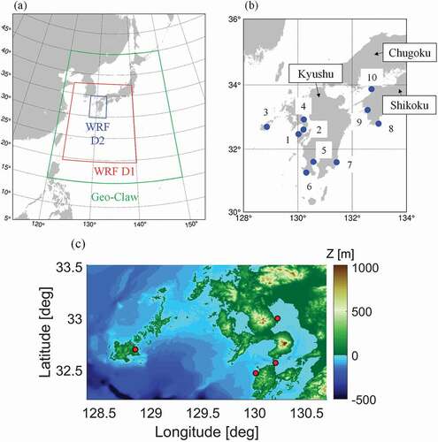
A coupled atmospheric-storm surge model was established by coupling the mesoscale meteorological model (WRF) and the storm surge model (GeoClaw). The coupled model was used to accurately simulate Typhoon Haishen and storm surges (Figure 1). Note that D2 (1 km) is a computational domain for confirming the reproducibility of the western Kyushu area. In addition, because the D2 area was too small to be used for storm surge simulations, D1 (5 km) was used.

Figure 1. Computational flow of hindcast experiment and forecast experiments.

2.1. Computational configuration for typhoons

The WRF model was used to simulate the meteorological field of typhoon (Table 1). It is a non-hydrostatic mesoscale model developed by the National Center for Atmospheric Research (NCAR; Skamarock et al.) and is used for a wide range of analyses of tropical cyclones (e.g. Ninomiya et al.). In this study, Typhoon Haishen was simulated with analysis and forecast data using the WRF model. We focused on quantitatively evaluating the forecast error of the storm surge caused by Typhoon Haishen and clarifying the characteristics of the forecast error by simulating the typhoon meteorological field with high accuracy during a storm surge.

Table 1. Computational settings for WRF

	Domain (D1)	Domain (D2)
TC Case	Typhoon Haishen (2020)
Period	12:00, September 2 2020–12:00, September 8 2020
Horizontal resolution	5 km	1 km
Horizontal grids	300 x 400	401 x 551
Time step	30 s	6 s
Vertical resolution	33 layers (1000–50 hPa)
Initialization	NCEP FNL (0.25°x 0.25°) NCEP GFS (0.25°x 0.25°)
Nudging	On (every 6 hours) Spectral nudging	Off
Cumulus convection scheme	Kain-Fritsch scheme (Kain 2004)	Off
Cloud microphysics scheme	WSM 6-class graupel scheme (Hong and Lim 2006)
PBL scheme	YSU scheme (Hong and Lim 2006)
Radiation scheme (long/short)	RRTMG scheme (Iacono et al. 2008)
Land-surface	5-layer Thermal diffusion scheme (Dudhia 1996)
Ocean physics	1d mixed layer model (Pollard and Thompson)

Two nesting domains (D1 and D2) were used as the WRF computational domain (Figure 2a, red and blue frames). D1 (5 km grid) is a domain that covers a wide area from the Kyushu region to western Japan and the surrounding sea area. D2 (1 km grid) was set up inside D1 and used to calculate the meteorological fields of storms in the Kyushu region with a higher resolution.

Figure 2. Simulation fields of WRF and GeoClaw. (a) Green line indicates the GeoClaw simulation area, red line indicates the WRF domain 1 simulation area, and blue line indicates the WRF domain 2 simulation area. (b) Blue points indicate storm surge observation sites. 1:Reihoku, 2:Kuchinotsu, 3:Fukue, 4:Oura, 5:Kagoshima, 6:Makurazaki, 7: Aburatsu, 8:Tosa-Shimizu, 9:Uwajima,10: Matsuyama. (c) This is topography data with 270 m resolution of GeoClaw. Red points are corresponding to No. 1–4 in (b).

In this study, a hindcast experiment on Typhoon Haishen and the storm surge was conducted first as a control run (hereafter, referred to as CNTL). Subsequently, forecast experiments were conducted under four conditions with different starting times: four days before (4 DB), three days before (3 DB), two days before (2 DB), and one day before (1 DB). The reference date and time was 12:00 UTC on September 6 2020, which is the time when Typhoon Haishen was closest to the Kyushu region. The simulated period of CNTL was from 12:00 UTC on September 2 2020, to 12:00 UTC on September 7 2020. The initial and boundary conditions were the final analysis data (FNL) of the National Centers for Environmental Prediction (NCEP) on a 0.25-degree grid. High-resolution merged satellite and in-situ data Global Daily Sea Surface Temperature (HIMSST) was used as the sea surface temperature (SST) data, which is interpolated every 6 h (original temporal interval is daily, and horizontal resolution is 0.1°). Although it is possible to use the SST from NCEP FNL, the accuracy of the simulations was higher with the HIMSST than with the FNL SST based on a preliminary analysis. Therefore, the NCEP FNL data were used as the atmospheric field, and the HIMSST was used as the SST in this study. For the forecast experiments, the NCEP Global Forecast System (GFS) data were used, and the start times were set to the specified number of days before the reference date and time (i.e. 12:00 UTC on September 2, 3, 4, and 5, 2020). The simulation end times were set to 12:00 UTC on September 7 2020, for 4 DB and 1 DB, and 00:00 UTC on September 8 2020, for 3 DB and 2 DB. This difference in the end time is due to the difference in the peak occurrence time caused by the moving speed of the typhoon at the time of each forecast. The forecast typhoon moved relatively slowly in the 3 DB and 2 DB simulations. Other details of the simulation settings are listed in Table 1. Here, the NCEP FNL and HIMSST are the reanalysis values. Thus, they cannot be used for real-time forecasting. On the other hand, the NCEP GFS is forecast data and can be used for real-time forecasting.

2.2. Computational configuration for the storm surge

2.2.1. Storm surge model

The storm surge model used in this study was GeoClaw, which was developed by Mandli and Dawson (2014). GeoClaw employs adaptive mesh refinement (AMR) algorithms that allow for the resolution of disparate spatial and temporal scales. GeoClaw solves the following nonlinear long-wave equations using the finite volume method based on the Riemann solver (details are provided in LeVeque 2002):

(1) $C_w=min\left(2\times {10}^{-3},\left(0.75+0.067\left|W\right|\times {10}^{-3}\right)\right)$(1)

In these equations, $C_w$ was empirically obtained from experiments, and Garratt’s drag formula (Garratt 1977), which was obtained by linear regression analysis using a wind speed at a 10 m altitude, as shown in Eq. (1)(1) $C_w=min\left(2\times {10}^{-3},\left(0.75+0.067\left|W\right|\times {10}^{-3}\right)\right)$(1) was used in this study. The value of the upper limit is not specified. The value of the friction coefficient $C_f$ was determined using the hybrid Chezy–Manning n-type friction law:

(2) $C_f=\frac{g{n}^2}{h^{\frac{4}{3}}}{\left[1-{\left(\frac{h_{break}}{h}\right)}^{{\theta }_f}\right]}^{{\gamma }_f/{\theta }_f},$(2)

where n denotes the Manning’s n coefficient [${\mathrm{m}}^{-\frac{1}{3}}{\mathrm{s}}^{-1}$] and $h_{break}=2$, ${\theta }_f=10$, and ${{\gamma }_f}_{=}4/3$ control the form of the friction law.

The patch-based AMR approach used in GeoClaw employs a set of overlapping logically rectangular grids that correspond to one of many levels of refinement that are enumerated starting at l = 1. The first of these levels contains grids that cover the entire domain at the coarsest resolution. The subsequent levels, i.e. $l\ge 2$, represent progressively finer resolutions by a set of prescribed ratios $r^l$ in time and space such that

(3) $\begin{array}{rl}& \mathrm{\Delta }{x}^{l+1}=\mathrm{\Delta }{x}^l/r_x^l,\\ & \mathrm{\Delta }{y}^{l+1}=\mathrm{\Delta }{y}^l/r_y^l,\\ & \mathrm{\Delta }{t}^{l+1}=\mathrm{\Delta }{t}^l/r_t^l\end{array}$(3)

The refinement criteria for the storm surge simulation include the wind speed and RMW based on the input meteorological field, in addition to the water level and flow velocity calculated at every time step.

2.2.2. Numerical setup

Storm surge simulations were performed for the northwestern Pacific Ocean and the coast of Japan (see the green frame in Figure 2). Table 2 presents an outline of the simulation settings. The simulation period was from the forecast start time (September 2, 3, 4, or 5 12:00 UTC) to September 7 2012:00 UTC (4 DB and 1 DB), and September 8 2000:00 UTC (3 DB and 2 DB). The storm surge simulation was validated at ten sites in Kyushu and western Shikoku (Figure 2b). The points where the maximum storm surge observed by the JMA exceeded 0.4 m were selected.

Table 2. Computational settings for GeoClaw, outline of the simulation settings

Period	12:00UTC, 2 – September 4 2020–12:00UTC, September 8 2020
Refinement level	[1,2,3,4]
Refinement ratio	[6,2,2]
Resolution [deg]	[1/10, 1/60, 1/120, 1/240]
Time step	Adaptive (CFL ≤0.5)
Wind drag coefficient	Garatt, 1977
Manning’s coefficient	Mandli and Dawson 2014

The 15 arc-second resolutions provided by the General Bathymetric Chart of the Oceans (GEBCO) were used for the topographic data (GEBCO 2020). On the coast of Japan, topographical data (resolutions: 2430 m, 810 m, 270 m; Figure 2c) published by the Central Disaster Prevention Council were used. GeoClaw can solve up to run-up. However, this model has problems such as not being able to include levees and not being able to handle the 0 m zone. In addition, the run-up was not included in the calculations in this study. The hydrostatic surface was 0 m, and tides were not considered. According to Mandli and Dawson (2014), Manning’s coefficient changes with water depth (Table 2). The refinement layers were levels 1 to 4 (maximum), and the refinement criteria are presented in Table 3. In GeoClaw, the computational time interval can be changed spatiotemporally according to the CFL condition. In this study, the computational time interval was changed such that the CFL was equal to or less than 0.5.

Table 3. Refinement criteria for the sea surface height T_wave, water speed T_speed, and wind speed T_wind. The lists of tolerances correspond to level criteria, i.e. the first entry is the tolerance for moving from levels 1 to 2

Criteria
Twave [m]	0.2
Tspeed [m/s]	1
Twind [m/s]	[20.0, 30.0, 40.0]

Storm surge simulations were performed with two different meteorological field models: the WRF model and the Holland model. Note that the storm translation speed is added to take into account the relative motion of the storm and atmosphere in the case of Holland model, and wind field is asymmetric. In Section 3, we compare forecast simulations in which the meteorological field of the WRF model is directly input to GeoClaw (coupled) and forecast simulations in which the initial values of the Holland model are input to the JMA forecast with no temporal change condition (PTC). In Section 4, the key parameters of typhoons are referenced to the WRF output, and the meteorological field is determined based on the parametric Holland typhoon model (Section 4). The simulation method is described in the next section.

2.3. Computational method of the Simple Ensemble Experiment for Storm Surge Forecast (SEES)

To evaluate the impact of different tracks on storm surge forecasts, the results of simple ensemble experiments for storm surge forecasting (SEES) assuming multiple typhoon tracks based on dynamic TC forecasts are discussed using the parametric Holland typhoon model to increase the number of TC tracks. In addition, the characteristics and limits of storm surge forecasts were determined. First, the simulation method of SEES is described. In this study, the Holland (1980) model, a parametric TC model for pressure and wind, was used to set up the meteorological field. The parametric typhoon model assumes an axis-symmetric pressure field given a minimum central pressure and RMW, and it has the advantage of arbitrary typhoon track translation and a very low computational cost. Therefore, the TC track ensemble can be easily considered using the parametric Holland typhoon model. This method is widely used by many municipalities in Japan for storm surge inundation assumptions (Ministry of Land, Infrastructure, Transport and Tourism 2020). However, it has a significant disadvantage: the dynamical and local characteristics of the typhoon, and the intensity and temporal changes in the RMW cannot be considered. In this study, the temporal changes in the typhoon intensity and RMW were considered using the hourly simulation result of the GFS obtained with the WRF model as the typhoon information for input into the parametric Holland typhoon model (Figure 3). Atmospheric pressure and wind speed, according to Holland (1980) in GeoClaw (Mandli and Dawson 2014) were used.

Figure 3. Computational flow of simple ensemble experiments for storm surge (SEES) .

The parametric Holland typhoon model requires information on the typhoon position (latitude and longitude), central pressure, maximum wind speed, and RMW. In this study, the results of forecast experiments (4 DB, 3 DB, 2 DB, and 1 DB) performed with the WRF model were used as the input conditions for the parametric Holland typhoon model. Furthermore, the output of the WRF model was used to obtain the values of the central pressure, maximum wind speed, and RMW (every hour). The SEES combines highly accurate meteorological model values with a low computational cost parametric model. Therefore, it is a realistic method in terms of both accuracy and computational cost.

Regarding the SEES, the perturbation of the track was set to 1°. Five types of typhoon track perturbations were considered: original track, 1-degree east, 1-degree west, 1-degree south, and 1-degree north. Therefore, storm surge forecasts were obtained for each day (4 DB, 3 DB, 2 DB, and 1 DB) using the five typhoon tracks and the same intensity and RMW (a total of 20 forecasts). The perturbation was chosen as 1° because the averaged error of JMA’s prior 24 h forecast of the typhoon track was estimated to be approximately 100 km (JMA 2020b, 2019). It should be noted that the typhoon track is shifted by 1° from start to end.

3. Pseudo-deterministic experiments based on the integrated atmosphere–storm surge coupled model

In this section, the results of the hindcast and pseudo-forecast experiments using the integrated atmospheric–storm surge model presented in Section 2 are discussed in Section 3.1 and Section 3.2, respectively.

3.1. Hindcast experiment for the storm surge

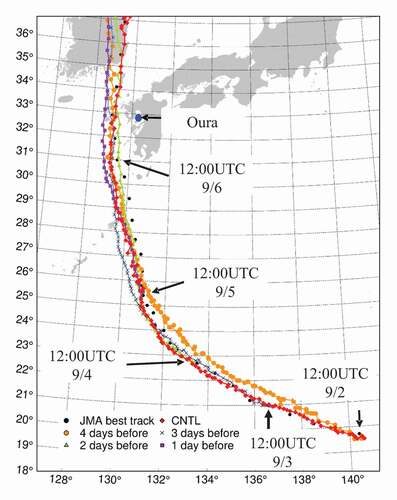
First, the intensity and track of Typhoon Haishen obtained with the WRF model utilizing the atmospheric analysis data were validated starting 00:00 UTC on September 6, as shown by the results of the CNTL in Figures 4 and 5, respectively (the other lines in the figure will be discussed in the next section). Because the output interval of the WRF is 1 h, the plot of each figure uses the same interval. According to the JMA best track data (observations; JMA 2020c), Typhoon Haishen developed with a minimum central pressure of 910 hPa on September 4. However, it approached Japan while rapidly weakening and moving northward over the western ocean of Kyushu (black line in Figure 4 and black dots in Figure 5). In the hindcast experiment (red line in Figure 4), the peak intensity of the CNTL was significantly underestimated by +20.5 hPa. This error is caused by the inability of the utilized model to capture the rapid intensification of typhoons in the FNL data as input and boundary conditions, and the large error in the parameterization of the WRF model at the time of typhoon intensification. However, the error decreased to 1.7 hPa when Typhoon Haishen approached the Kyushu region. Regarding the accuracy of the typhoon track (Figure 5), the period near the Nansei Islands was temporarily shifted to the west by approximately 40 km. However, the error was less than 20 km after 00:00 UTC on September 6, indicating that the accuracy of the model had improved. The observed moving speed when going north to the west of Kyushu was 34.8 km/h, and the result of the WRF model was 31.6 km/h. Although the moving speed tended to be underestimated, the typhoon movement could be expressed accurately. A relatively accurate typhoon track can be simulated in the later period of Typhoon Haishen because of the spectral nudging applied to the CNTL.

Figure 4. Time series of central pressure for Haishen (2020). Black line is JMA best track, the red diamond line is hindcast simulation (CNTL), the Orange circle line is 4 days before, the blue X line is 3 days before, the green triangle line is 2 days before, and the purple square line is 1 day before. Note that Orange, blue, green, and purple lines are the results of forecast experiments. The vertical axis represents the central pressure of the typhoon, and the horizontal axis represents the time; the typhoon attenuates from left to right.

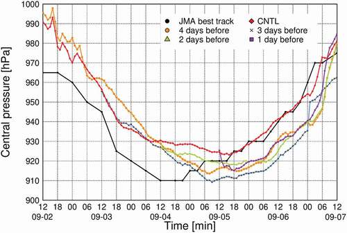
Figure 5. Typhoon tracks simulated by WRF. Each line color follows Figure 4. The symbols plotted in every hour constantly. Blue point indicates the port of Oura. The daily typhoon positions by JMA best track are also shown.

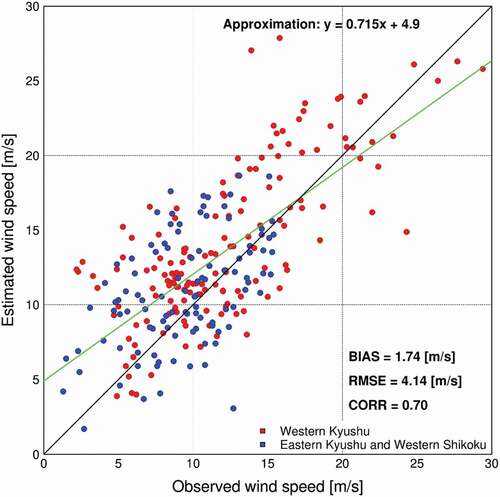
Subsequently, the accuracy of the wind speeds in the Kyushu region and western Shikoku was validated against in situ data, as shown in Figure 6. The observed data of 20 sites (12 sites on the west coast of Kyushu, eight sites on the east coast of Kyushu, and western Shikoku) in the JMA Automated Meteorological Data Acquisition System (AMeDAS) were used for validation (18:00 UTC on September 6 to 06:00 UTC on September 7). The bias and root mean square errors (RMSE) were 1.74 m/s and 4.14 m/s, respectively, both of which are small. The correlation coefficient was 0.70, and there were no significant differences in the correlation between the eastern and western parts of Kyushu. Strong winds exceeding 20 m/s could be simulated along the west coast of Kyushu near the side of the typhoon track (red dots in Figure 6), and slower winds below 10 m/s at the sites on the east coast of Kyushu and western Shikoku (blue dots in Figure 6), which are far from the typhoon, could also be reproduced.

Figure 6. Scatter plot of wind speeds observed in Kyushu and western Shikoku and wind speeds by WRF. The red dots represent the values in western Kyushu near the typhoon, and the blue dots represent the values in eastern Kyushu and western Shikoku. BIAS represents the bias error, RMSE represents the root mean square error, and CORR represents the correlation coefficient. The black line represents y = x and the green line represents the regression line.

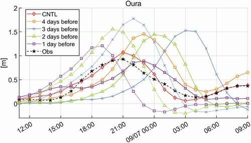
Finally, the accuracy of the storm surge height was validated using the tidal gauges shown in Figure 7. Figure 7 shows the time series of the storm surge height for the observed data (black dashed line) and the CNTL (red line) at the Port of Oura in Saga Prefecture. Two types of tide observation data can be obtained from JMA: a 3-min mean value and an hourly mean value. However, the 3-min mean value was not published, except for the peak time. Therefore, the hourly observation value, including the data before and after the genesis of the storm surge, were used for the validation. The storm surge discussed in this manuscript is the sea level anomaly, and the tide was removed from the storm surge values. The observed and simulated maximum storm surge heights at the Port of Oura were 0.93 m and 1.07 m, respectively. Thus, the maximum storm surge height could be reproduced at this location. Although the time series of the observed and simulated sea surface elevations were similar, their peak times lagged by approximately 1 h. The reason for the time lag is the accuracy of the typhoon translation speed and the trend of the CTNL being slower than the observed trend.

Figure 7. Time series of storm surges at the Port of Oura. The vertical axis represents the height of the storm surge, and the horizontal axis represents time. The color solid lines indicate the results of WRF-GeoClaw coupled model, and the color dashed lines indicate the results of PTC model. Each line color follows .Figure 4

The accuracy of the TC characteristics and related storm surges were analyzed. This is the best performance of the hindcast experiments using the integrated atmosphere-storm surge model. The accuracy of the storm surge forecast will be discussed in the following sections.

3.2. Pseudo forecast experiments for the storm surge

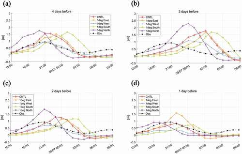
The results of the forecast experiments performed with the coupled model using the NCEP GFS data as the initial and boundary values were compared with the CNTL run and observed data, as shown in Figures 4 and 5, respectively. In this study, four types of forecast experiments using WRF-GeoClaw (Coupled) were conducted with different starting times for the computation: four days before (4 DB; orange), three days before (3 DB; blue), two days before (2 DB; green), and one day before (1 DB; purple) the typhoon event. It was observed that the typhoon intensity in the forecast simulations showed a tendency to be stronger than that in the CNTL. Additionally, the peak times of the forecast simulations were 24 h later than the observed peak times. The result of the 4 DB forecast was the closest to the CNTL in terms of typhoon intensity, although the peak time appeared later. On September 6, when the typhoon faded and approached Japan, the average typhoon intensity was stronger – 10.9 hPa than that obtained in the CNTL (00:00 UTC on September 6). Regarding the typhoon track, the 4 DB and 3 DB forecasts have almost the same track as the CNTL, whereas the 2 DB has a track that is approximately 20 km eastward, and the 1 DB has a track that is approximately 30 km westward (average value from 18:00 UTC on September 6 to 06:00 UTC on September 7). Additionally, there was a significant difference in 3 DB and 2 DB forecast case at the time of the typhoon approaching Japan. The approach times for the 4 DB and 1 DB forecasts were almost the same as that of the CNTL, whereas the approach times for the 3 DB and 2 DB were 3–4 h behind than observed the approach time of the typhoon to Japan. Although almost no difference in the moving speed of the typhoons after September 6 was observed, there was a significant difference before the typhoon approached Japan. This is because the typhoon’s northward speed was approximately 10 km/h slower than the actual speed in the southern area of 25°N in the GFS used as the initial value in 2 DB and 3 DB forecasts. This error was presumed to cause a time error in the maximum storm surge. As a result, the 4 DB forecast had the smallest error with respect to the typhoon intensity and tracks. Thus, the 1 DB forecast was not the most accurate forecast for typhoon intensity and track. Even the most recent 24 h advance track forecast by the general circulation model contains a forecast error of approximately 80 km (Japan Meteorological Agency 2020e). Therefore, the deviation of the track in the 1 DB and 4 DB forecasts is within the range of the JMA’s 24 h advance error. As a result, the 4 DB forecast was the most accurate, and the 1 DB forecast was the second most accurate. The track forecast error can be considered by performing an ensemble simulation by slightly changing both the initial and boundary conditions, as in Toyoda, Yoshino, and Kobayashi .

Next, the results of the storm surge forecast simulations are discussed based on Figure 7 and Table 4. In all three forecast results, except the 1 DB forecast, the maximum storm surge in Oura was overestimated compared to the CNTL (ratio): + 0.38 m (+ 36%), + 0.46 m (+ 43%), and + 0.37 m (+ 35%) in the 4 DB, 3 DB, and 2 DB forecasts, respectively. The 1 DB is the only forecast that was underestimated by – 0.18 m (–16%) and exhibited the smallest error relative to the CNTL. The accuracy of the peak times decreased in the order of 1 DB, 4 DB, 2 DB, and 3 DB. In the 1 DB forecast, the peak time was delayed by 2 h, and in the 3 DB, there was a delay of 6 h. Based on the absolute error of the peak storm surge, the 1 DB can express a realistic storm surge, although it appears that the typhoon track is off to the west.

Table 4. Summary of results of storm surge forecast simulation by atmosphere-storm surge coupled model. CNTL is the hindcast simulation result. Based on September 6 2020, it is defined as 4 days before, 3 days before, 2 days before, and 1 day before

	Peak time (UTC)	Maximum storm surge (m)
CNTL	9/6 21:00	1.07
4 days before	9/6 23:00	1.45
3 days before	9/7 3:00	1.53
2 days before	9/7 0:00	1.45
1 day before	9/6 23:00	0.89

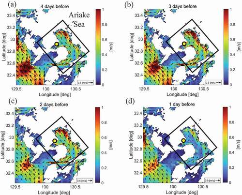
We now discuss the results of the comparisons between the forecast experiments based on the results of the 1 DB forecast, which had the highest accuracy in forecasting the storm surge. The 1 DB forecast (0.89 m) had the same scale as the observed storm surge (0.93 m), but the other three cases were overestimated by approximately 0.60 m. Furthermore, there was almost no difference in the typhoon intensity, moving speed, and the peak time of storm surge between the 1 DB and 4 DB forecasts. However, the 4 DB forecast was close to the observed track, and the 1 DB had a track of approximately 30 km westward. Based on the difference between the 1 DB and 4 DB forecasts, the contribution of typhoon track errors to the scale of storm surge was estimated as 0.60 m. It is coincidental that the scale of the storm surge was properly forecast in the 1 DB forecast. If the typhoon track of 1 DB was forecasted as observed, the storm surge forecast was also overestimated, as in 4 DB. The storm surge forecasts were overestimated in the 4 DB, 3 DB, and 2 DB forecasts because the typhoon intensities when the typhoons were closest to Japan were overestimated in all cases. Comparing the 4 DB forecast and the CNTL, the error source of the typhoon intensity in the peak storm surge forecast was estimated as about 0.40 m because the two forecasts had similar values except for the typhoon intensity. However, although the intensity was overestimated in the 1 DB forecasts, it is comparable to that of the storm surge forecast because of the westward shift of the typhoon’s track. According to the maximum flow velocity distribution during the computational period centered on the Ariake Sea (Figure 8), a large and similar amount of seawater was moved from the south to the north in the Ariake Sea and Oura in the 4 DB, 3 DB, and 2 DB forecasts. However, the current was slower in the 1 DB forecast, where the typhoon track was shifted by approximately 30 km west, causing a reduction in the regional scale of the storm surge because of a weakening of the winds over the Ariake Sea. As a result, the 1 DB forecast had the same scale as the observed storm surge. From these results, the error source of the typhoon track on storm surge was approximately 0.60 m (the difference between 1 DB and 4 DB), and the error source of the typhoon intensity on storm surge was approximately 0.40 m (the difference between CNTL and 4 DB). Therefore, the impact of the typhoon track was 1.5 times larger than the impact of the typhoon intensity. This result is consistent with the results of a previous study (Mori et al.) that the forecast error of the storm surge by the typhoon track is larger than that of the typhoon intensity. However, these results are valid only for Typhoon Haishen, and it is necessary to perform the same validation in different cases to obtain more robust values.

Figure 8. Differences in the maximum flow velocity of seawater flowing to the Ariake Sea between (a) 4 DB, (b) 3 DB, (c) 2 DB, and (d) 1 DB. Ariake Sea is indicated inside the black line, and yellow point means the Port of Oura. The color bar shows the flow velocity, blue is low flow velocity and red is high flow velocity.

Next, we compare the results of the forecast simulations using the Holland model (PTC, Figure 7; dashed lines), which is used in practice, with those using the coupled model (Figure 7; solid lines). The forecast values by JMA (3 DB, 2 DB, and 1 DB) were used for the input condition of PTC location and intensity. The RMW value was set to 70 km based on the satellite estimation value by NOAA. The results of both methods revealed that the accuracy of the storm surge scale generally tends to improve as the forecast period becomes shorter. Comparing the results for the same date, the coupled simulation has a higher accuracy in the storm surge scale. The PTC overestimates the storm surge by about 0.30 m (30%, even with a one-day advance forecast), while the coupled model forecasts a storm surge of a reasonable value based on the observed value. This is because the PTC does not take into account the attenuation of the typhoon, which shows the limitation of this method. On the other hand, the peak time forecast tends to be different from the scale forecast, and the PTC is closer to the 3 DB and 2 DB forecasts. This is due to the error caused by the delay in the approach time of the typhoon in the initial and boundary values input to the WRF in the coupled model. Therefore, it is necessary to prepare a large number of tracks to account for uncertainty in the forecast error. In this case, the typhoon track was a straight line from south to north, and PTC was able to calculate it with high accuracy (especially the peak time of storm surge). However, the error is likely to be larger when the track is more complicated, such as when it is a curved line.

4. Results and discussion of SEES

In the previous section, we described the WRF-GeoClaw coupled calculations and parametric model simulations that were performed. Although the coupled simulation has a high computational cost, it can represent a realistic storm surge. However, the PTC tends to overestimate the storm surge, and this model has poor accuracy. In this section, we propose a method that can be used by practitioners to reduce computational cost while ensuring accuracy by applying the WRF output to the parametric model. We evaluate the practicality and limitations of this method using simple ensemble experiments for storm surge forecasting (SEES).

First, as in the previous section, we confirmed the time series of the storm surge height in Oura (Figure 9). In any simulation of the 4 DB-1 DB, the peak time is the earliest in the case of 1-degree north. The case of 1-degree north shows the largest maximum storm surge height in all three cases except the 1 DB forecast. The initial position shift of the typhoon to the north caused an approach to western Kyushu before the typhoon intensity weakened. The largest peak storm surge height in the 1 DB forecast was in the case of 1-degree east. The typhoon track was shifted to the west by approximately 30 km in the WRF simulation results for the 1 DB. Hence, the shift of the track to the east caused the Ariake Sea to become located near the RMW of the typhoon. Therefore, a stronger wind flow to the Ariake Sea led to significant increases in storm surge heights. The peak times and maximum storm surge fluctuated in the range of 5 h and 1.0 m, respectively, for the five typhoon tracks in Oura.

Figure 9. Time series of storm surges at the Port of Oura by SEES ((a) 4 DB, (b) 3 DB, (c) 2 DB, and (d) 1 DB). The vertical axis represents the height of the storm surge, and the horizontal axis represents time. The red diamond line is original from the WRF results, the Orange circle line represents moving the typhoon track east at 1 degree, the blue X line represents moving the typhoon track west at 1 degree, the green triangle line represents moving the typhoon track south at 1 degree, and the purple square line represents moving the typhoon track north at 1 degree.

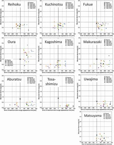
Storm surges were forecasted in western and eastern Kyushu, and parts of the Chugoku-Shikoku region, which is far away from the typhoons. There were ten tidal gauges affected by Typhoon Haishen in the Kyushu and Chugoku-Shikoku regions (Figure 2). The maximum storm surge heights and peak occurrence times were compared between the SEES and gauge data, as shown in Figure 10. Note that the observed values in this discussion are the average values for the 3-min observations published by JMA, which are different from the 1-hour observed values used in the time series analysis. The vertical axis in Figure 10 represents the maximum storm surge height at each site. The X, star, and horizontal axes represent the observed value, ensemble mean of SEES, and peak time error relative to the observed value, respectively. Note that, for Tosa-Shimizu and Uwajima, in some cases, the maximum values were recorded more than 1.5 days (2160 min) before observed peak. However, the errors were too large to be represented on the same axis. Therefore, Figure 10 does not show errors of more than 720 min. Comparing the observed values with the ensemble mean in Figure 10, the peak intensity and time of the storm surge can be forecast with high accuracy in Reihoku and Kuchinotsu because X and Star are close to each other (within 20% error). In Fukue and Oura, the storm surge height errors are 0.16 m and 0.37 m, respectively. On the other hand, the peak time errors shown in Figure 10 are forecasted as 221 and 303 min, respectively, which are significant delays. Therefore, the tendency of maximum storm surge forecast errors is small at Reihoku and Kuchinotsu, which are close to the typhoon center, and large at other sites (especially Aburatsu, Matsuyama, Uwajima, and Tosa-Shimizu, which are farther from the typhoon). At all the simulation sites, at least one member shows the error of the peak time of the storm surge less than a certain minute. However, no ensemble member was successful in accurately forecasting the maximum storm surge height at a site far from the typhoon center.

Figure 10. Scatter plot of maximum storm surge occurrence time error and storm surge deviation at each site. Orange is the result of 4 DB, blue is 3 DB, green is 2 DB, and purple is 1 DB. The shape of the symbol is the same as that in Figure 9. X represents the observed value, and the star represents the average value of all cases. Note that the results are not displayed in the figure for simulations with a time error of 720 minutes or more.

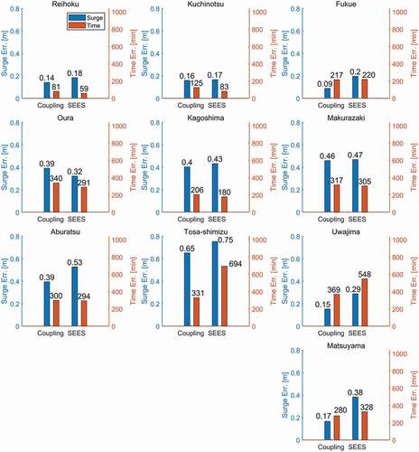
Next, we focus on the variations in the peak time error and maximum storm surge errors at each site (Figure 11). Figure 11 shows the absolute average error of the WRF-GeoClaw coupled simulation and SEES results. The averages were weighted according to the forecast time, and the weight was increased for the 1 DB forecast. In Reihoku, which has the best forecast accuracy, the average time error is 59 min and the average storm surge error is 0.18 m. On the other hand, in Tosa-Shimizu, which has the worst accuracy, the average peak time error is 694 min and the storm surge error is 0.75 m. Both the coupled model and SEES tend to have smaller errors at sites close to the typhoon and larger errors at the sites that are far from the typhoon. The large errors in the storm surge scales for Makurazaki and Tosa-Shimizu are due to the relatively large storm surges that occurred and the smaller simulated values. Although the mean error of SEES is larger than that of the coupled model, the trend of the error is similar between the coupled model and SEES, indicating that the accuracy of SEES storm surge forecasting can be ensured even though it is based on a parametric model. The accuracy of the storm surge scale by SEES was improved compared to using only the parametric typhoon model. As shown in Figure 10, all the sites contain at least one case out of the 20 cases that exhibits a peak time close to the observed peak time, and it is possible to forecast the peak time regardless of the distance from the center of the typhoon to the target site. In other words, the peak of the storm surge can be forecast regardless of the distance from the typhoon in several cases. However, in the maximum storm surge forecast, almost all the cases were underestimated by 40% or more except for the four cites (Reihoku, Kuchinotsu, Fukue, and Oura).  Therefore, there a successful forecast (e.g., within 10% error) of the maximum storm surge were not obtained. Thus, the performance of the SEES is more superior to that of the WRF-GeoClaw coupled model in forecasting the peak time of the storm surge than in forecasting the maximum storm surge height. Furthermore, the usefulness of the SEES for translation of the track is effective at sites near the typhoon (western Kyushu), and only the peak time forecast is effective at sites far from the typhoon. In addition, even at sites close to the typhoon, the variability of each case tends to be greater in the inner bays (e.g. Oura) than in the bays facing the open ocean. The impact of typhoon tracks on storm surges is greater in inner bays than in bays facing the open ocean. In this study, we used the results of four WRF simulations to perform 20 track ensemble forecasts of storm surges. If a greater number of WRF simulations can be performed, the SEES method may be able to accurately forecast the scale of storm surges at sites far from the typhoon.

Figure 11. The averages of the error by WRF-GeoClaw coupled model and SEES for the 10 sites of the storm surge calculation. Blue and red indicate maximum storm surge error and peak time errors, respectively, with the left and right vertical axes corresponding to storm surge error and time error.

5. Conclusions

In this study, hindcast and pseudo-forecast experiments using an atmosphere-storm surge-coupled model for Typhoon Haishen (2020) were conducted. The results revealed that the impact of the forecast error of the typhoon track on the storm surge forecast error is approximately 1.5 times greater than that of the typhoon intensity. Note that this result was obtained for Typhoon Haishen, and similar studies are needed to accumulate cases. In addition, a comparison between the parametric Holland (1980) model, which is commonly used by practitioners, and the coupled model revealed that the Holland model tends to overestimate the storm surge. Therefore, it is necessary to reduce or include typhoon track forecast errors in forecasting models to improve storm surge forecasts.

In addition, the parametric Holland typhoon model was able to accurately forecast the storm surge height near the typhoon and its peak occurrence time. However, the forecast accuracy tended to decrease as the distance from the typhoon to the target location increased. We performed a simple ensemble storm surge forecast considering the uncertainty of the typhoon track forecast. The results of the 20 ensemble forecast simulations revealed that the perturbed typhoon track simulation can increase the possibility of capturing the peak time of the storm surge. In other words, although the ensemble track experiment improves the forecast for the peak time of the storm surge, there is little improvement in the forecast for the scale of the storm surge. This problem can be solved by conducting ensemble experiments with intensities other than the track. In addition, the perturbation of the track ensemble was given as 1°. In future studies, perturbations corresponding to the forecast period and typhoon intensities will be used to improve the SEES method. Moreover, both the maximum storm surge and peak time in the track ensemble experiments were more sensitive in the inner bay than in the open ocean. In this study, we performed 20 track ensemble storm surge forecasts using four WRF simulation cases. In the future, more robust results could be obtained by conducting track ensemble experiments based on more WRF simulations and by targeting typhoon cases with different characteristics.

Acknowledgments

This research work was supported by two JSPS Research Fellow Grants (No. 20J00218 and No. 19J22429) and a JSPS Grant-in-Aid for Scientific Research (A) (No. 19H00782).

Disclosure statement

No potential conflict of interest was reported by the author(s).

Additional information

Funding

This work was supported by the Japan Society for the Promotion of Science [20J00218]; Japan Society for the Promotion of Science [19H00782]; Japan Society for thePromotion of Science [19J22429].

References

- Dudhia, J. 1996. “A Multilayer Soil Temperature Model for MM5.” Preprints, Sixth PSU/NCAR Mesoscale Model Users’ Workshop, Boulder, CO, PSU/NCAR, 49–50.
- Feng, X., M. Li, B. Yin, D. Yang, and H. Yang. 2018. “Study of Storm Surge Trends in Typhoon-prone Coastal Areas Based on Observations and Surge-wave Coupled Simulations.” International Journal of Applied Earth Observation and Geoinformation 68: 272–278. doi:https://doi.org/10.1016/j.jag.2018.01.006.
- Garratt, J. R. 1977. “Review of Drag Coefficients Over Oceans and Continents.” Monthly Weather Review 105 (7): 915–929.
- GEBCO Compilation Group. 2020. “GEBCO 2020 Grid.” doi:https://doi.org/10.5285/a29c5465-b138-234d-e053-6c86abc040b9.
- Holland, G. J. 1980. “An Analytic Model of the Wind and Pressure Profiles in Hurricanes.” Monthly Weather Review 108 (8): 1212–1218. doi:https://doi.org/10.1175/1520-0493(1980)108<1212:AAMOTW>2.0.CO;2.
- Hong, S. Y., and Lim, J. O. J. 2006. “The WRF Single Moment 6 Class Microphysics Scheme (WSM6).” Journal of the Korean Meteorological Society 42: 129–151.
- Iacono, M. J., J. S. Delamere, E. J. Mlawer, M. W. Shephard, S. A. Clough, & W. D. Collins. 2008. “Radiative Forcing by Long-Lived Greenhouse Gases: Calculations with the AER Radiative Transfer Models.” Journal of Geophysical Research 113: D13103.
- Iwamoto, T., R. Nakamura, T. Oyama, R. Mizukami, and T. Shibayama. 2014. “Prediction of Storm Surge at Tokyo Bay under RCP8.5 Scenario by Using Meteorological-Surge-Tide Coupled Model.” Journal of Japan Society of Civil Engineers, Series B2 (Coastal Engineering) 70 (2): 1261–1265. doi:https://doi.org/10.2208/kaigan.70.I_1261.
- Japan Meteorological Agency. 2018. “Information of Typhoon No. 24 (Sep. 3, 2018).” Press release material, 15.
- Japan Meteorological Agency. 2019. “Heavy Rain, Storm, etc. Due to Typhoon No. 19.” 65.
- Japan Meteorological Agency. 2020a. “Heavy Rains and Storms Caused by the Boso Peninsula Typhoon in the First Year of Reiwa and Its Fronts from August 13 to September 23, Etc.” Meteorological report at the time of disaster, 293.
- Japan Meteorological Agency. 2020b. “Typhoon Forecast Accuracy Verification Results.” Accessed 8 February 2021. https://www.data.jma.go.jp/fcd/yoho/typ_kensho/typ_hyoka_top.html
- Japan Meteorological Agency. 2020c. “Typhoon Position Table Reiwa 2nd Year (2020).” Accessed 8 February 2021. https://www.data.jma.go.jp/fcd/yoho/typhoon/position_table/table2020.html
- Japan Meteorological Agency. 2020d. “Storm, Heavy Rain, etc. Due to Typhoon No. 10.” Weather cases that caused disasters, 47.
- Japan Meteorological Agency. 2020e. “Verification of Forecast for Typhoon No. 10 in 2nd Year of Reiwa.” Press release material, 4.
- Japan Weather Association. 2018. “The Highest Tide in the Tokai Region Is Comparable to the Isewan Typhoon.” Accessed 8 February 2021. https://tenki.jp/forecaster/k_shiraishi/2018/09/30/2243.html
- Kowaleski, A., R. Morss, D. Ahijevych, and K. Fossell. 2020. “Using a WRF-ADCIRC Ensemble and Track Clustering to Investigate Storm Surge Hazards and Inundation Scenarios Associated with Hurricane Irma.” Weather and Forecasting 35 (4): 1289–1315. doi:https://doi.org/10.1175/WAF-D-19-0169.1.
- Ministry of Land, Infrastructure, Transport and Tourism, Japan. 2020. “Storm Surge Inundation Assumption Area Figure Making Manual(Ver.2.00).” 84.
- LeVeque, R. 2002. Finite Volume Methods for Hyperbolic Problems, Cambridge Texts in Applied Mathematics. Cambridge, UK: Cambridge University Press.
- Mandli, K. T., and C. N. Dawson. 2014. “Adaptive Mesh Refinement for Storm Surge.” Ocean Modelling 75: 36–50. doi:https://doi.org/10.1016/j.ocemod.2014.01.002.
- Mattocks, C., and C. Forbes. 2008. “A Real-time, Event-triggered Storm Surge Forecasting System for the State of North Carolina.” Ocean Modelling 25 (3–4): 95–119. doi:https://doi.org/10.1016/j.ocemod.2008.06.008.