 ?Mathematical formulae have been encoded as MathML and are displayed in this HTML version using MathJax in order to improve their display. Uncheck the box to turn MathJax off. This feature requires Javascript. Click on a formula to zoom.
ABSTRACT
The purpose of these comments and discussion has been to demonstrate how wave statistics can be incorporated into future applications of the proposed empirical equations to estimate the maximum relative uplift pressure under positive and negative freeboards on berm revetment with Seabee slope. This is demonstrated by using a joint distribution of significant wave height and surf parameter as well as by giving examples of the results.
1. Discussion
First, the discussers wish to compliment the authors, Zhou et al. (Citation2020) (hereafter referred to as Z20), on their results proposing empirical equations to estimate the maximum relative uplift pressure under positive and negative freeboards on berm revetment with Seabee slope. The empirical equations were obtained as best fit to data from laboratory tests in model scale 1:14 representing irregular wave conditions. Overall, the uneven distribution of the uplift pressure on this revetment structure would affect its stability and cause damage. These comments and discussion have been written to demonstrate how wave statistics can be incorporated into future applications of the authors’ empirical equations.
Z20 defined the dimensionless parameter
representing the 1% relative uplift pressure, where is the uplift pressure level exceeded by 1% of the measured time series,
is the fluid density, g is the acceleration due to gravity, and
is the significant wave height. The following empirical equations to estimate the maximum relative freeboard on berm revetment with Seabee slope were proposed:
For negative freeboard:
For positive freeboard:
where is the influence parameter of the elevation of the berm expressed in terms of the relative freeboard
, and
is the freeboard of the berm. Moreover,
is the surf parameter defined as
where
is the slope with an angle
to the horizontal,
is the deep water spectral wave length,
is the spectral period, and
is the deep water significant wave height. EquationEquations (1
(1)
(1) ) to (Equation6
(6)
(6) ) were obtained as best fit to data obtained in physical model tests performed in a wave flume using irregular waves in model scale 1:14 (see Z20 for more details).
The statistical features of (and thus of
) will be exemplified based on wave statistics obtained from the joint probability density function (pdf) of
and
provided in the Appendix, which is based on data from wave measurements made in the Northern North Sea during a 29 years period. Here, the conditional expected value of
given
and the conditional variance of
given
,
are considered.
Based on EquationEquations (4)(4)
(4) and (Equation6
(6)
(6) ),
is valid within a finite interval, and thus, the conditional pdf of
given
,
in EquationEquation (A2)
(A2)
(A2) in the Appendix follows the truncated lognormal pdf
where is the standard Gaussian cumulative distribution function (cdf) (where
and
are the mean value and the variance, respectively, of
) given by
It should be noted that the interval limits and
in EquationEquation (7)
(7)
(7) are based on the results depicted in Fig. 13 of Z20 (i.e. slightly extending the interval in EquationEquation (4)
(4)
(4) ). Further details of
are given in EquationEquations (A2
(A2)
(A2) ) to (EquationA6
(A6)
(A6) ) in the Appendix.
First, define
Then, the conditional expected value of P given ,
and the conditional variance of P given
,
are calculated from the truncated pdf of
given
in EquationEquations (7)
(7)
(7) and (Equation8
(8)
(8) ) as (Bury Citation1975)
where
The conditional coefficient of variation is
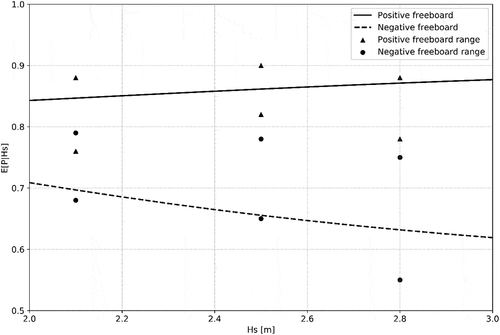
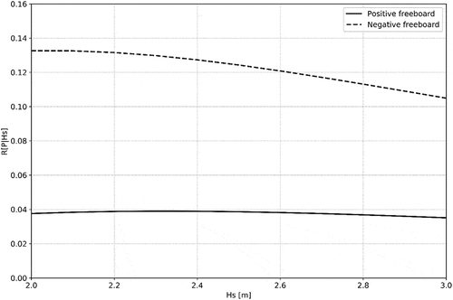
depict () and
() for the negative and positive freeboards versus
in the range 2– 3 m. This interval of
includes the full scale values
= 2.1 m, 2.5 m, 2.8 m corresponding to the model scale (1:14) values
= 0.15 m, 0.18 m, 0.20 m, respectively (see Z20). Here and in the following examples, the slope
is taken as 1:3 (as in Z20).
Figure 1. versus
for negative and positive freeboards with slope 1:3.

From , it appears, as increases from 2 m to 3 m, that:
increases from about 0.84 to about 0.88 for positive freeboard; and decreases from about 0.71 to about 0.62 for negative freeboard. The Z20 data representing the full scale values
= 2.1 m, 2.5 m, 2.8 m corresponding to
= 2.04, 1.86, 1.77, respectively, using
, are also shown for the positive and negative freeboard ranges taken from Fig. 13 in Z20. It appears that the two curves are within the ranges of the corresponding data.
From , it appears, as increases from 2 m to 3 m, that:
varies slightly from about 0.038 to about 0.035 with a maximum of about 0.039 for
= 2.3 m for positive freeboard; and decreases from about 0.133 to about 0.105 for negative freeboard.
Furthermore, examples of physical results are provided for negative and positive freeboards using the results in . Combination of EquationEquations (1)(1)
(1) , (Equation10
(10)
(10) ) and (Equation11
(11)
(11) ) yields
First, for negative freeboard:
Taking in EquationEquation (3)
(3)
(3) gives
which substituted in EquationEquation (15)
(15)
(15) for
= 2.5 m,
= 1025 kg/m3 and
(see ) yields
Furthermore, now (see ), and thus
plus and minus one standard deviation of 12.4% become
and
, respectively.
Second, for positive freeboard:
Taking in EquationEquation (5)
(5)
(5) gives
which substituted in EquationEquation (15)
(15)
(15) for
(see ) yields
Furthermore, now (see ), and thus
plus and minus one standard deviation of 3.9% become
and
, respectively.
Thus, as expected, these examples demonstrate that the wave-induced uplift pressure on berm revetment with Seabee slope is larger under positive freeboard than under negative freeboard.
In future applications of the empirical equations to estimate the maximum relative uplift pressure under positive and negative freeboards on berm revetment with Seabee slope proposed by Zhou et al. (Citation2020), it should be considered to implement the statistical properties of waves as demonstrated in this discussion, although the proposed equations and parameters may be subject to regional limitations. The utilization of these empirical equations jointly with wave statistics should represent an important component in, for instance, risk analysis used as part of revetment structure design. It should be noted, however, that implementation of wave statistics is not limited to the joint distribution of significant wave height and surf parameter applied here.
Disclosure statement
No potential conflict of interest was reported by the author(s).
References
- Bury, K.V. 1975. Statistical Models in Applied Science. New York: John Wiley & Sons.
- Myrhaug, D., and S. Fouques. 2010. “A Joint Distribution of Significant Wave Height and Characteristic Surf Parameter.” Coastal Engineering 57 (10): 948–952. doi:https://doi.org/10.1016/j.coastaleng.2010.05.001.
- Zhou, Z., Y. Chen, Y. Pan, Y. Shen., and M. Gan. 2020. “Wave-induced Uplift Pressure on Berm Revetment with Seabee Slope.” Coastal Engineering Journal 62 (4): 527–539. doi:https://doi.org/10.1080/21664250.2020.1816527.
Appendix.
Joint pdf of 
 and
and 

Here, the joint pdf of and
provided by Myrhaug and Fouques (Citation2010) (hereafter referred to as MF10) is used as an example. This
distribution was deduced based on a joint pdf of
and
obtained as a best fit to data from wave measurements made in the Northern North Sea during a 29-year period. The joint pdf of
and
is given as
where is the marginal pdf of
given by the combined lognormal and Weibull distribution given in EquationEquations (2
(2)
(2) –Equation4
(4)
(4) ) in MF10. The conditional pdf of
given
is given by the following lognormal distribution
where and
are the mean value and the variance, respectively, of
, given by
with
where is in meters in EquationEquations (A3)
(A3)
(A3) and (EquationA4
(A4)
(A4) ) (see MF10 for more details).

