A 3D numerical study on tsunamis ascending a river

ABSTRACT

Three-dimensional numerical simulations were generated for tsunamis ascending processes with different river topographies. As tsunamis propagated in a narrow river, the radius of curvature around the first wave peak decreased, increasing the tsunami height with wave disintegration until the second tsunami height peak appeared. The diffracted waves also entered the river channel, causing an increase in tsunami height in the vicinity of the riverbank at the estuary. The tsunami height increased in a uniform riverbed gradient and narrower river width toward the upstream, based on the shallowing and energy concentration. As the angle between the riverbank line and coastline at the estuary was acute, the tsunami height was reduced because the diffracted waves were difficult to enter the river. The tsunami height in the rivers increased as the ratio of representative wavelength to river width was increased. The maximum tsunami height in the bore-shaped wave was larger than in the solitary wave with the same incident wave height. In the case of tsunami propagation in the compound cross-section river, multiple crestlines appeared because the tsunamis traveling diagonally in the flood channel showed multiple reflections both on the riverbank and between the flood and main channels.

KEYWORDS:

• Tsunami
• river
• wave disintegration
• compound cross-section
• 3d numerical calculation

1. Introduction

The 2011 Great East Japan earthquake triggered huge tsunamis, causing enormous damage to the riverside areas in many rivers by the processes of tsunami run-up and river embankment overflow (e.g. Kakinuma et al. 2012). In the Kitakami River, a series of shock waves, namely tsunami bores, at approximately one-minute time intervals were recoded near a weir at 17.2 km from the estuary. The tsunami bores kept their wave shape over a distance of 10.9 km (Tolkova and Tanaka 2016). The tsunamis traveling along rivers have been investigated in several earthquakes including the 1983 Sea of Japan earthquake (Shuto 1985), the 2003 Tokachi-oki earthquake (Yasuda 2010), the 2004 Indian Ocean earthquake (Tanaka et al. 2008), and the 2010 Chile earthquake (Fritz et al. 2011). The tsunamis ascending a river generally show a larger phase velocity and longer run-up distance than the on-land tsunamis. Therefore, river tsunamis could damage the upstream river areas far from coasts. Countermeasures against river tsunamis have become urgent and received the attention of many government organizations, e.g. State of Oregon Department of Geology and Mineral Industries (2021) and River Tsunami Countermeasures Study Group (2011).

Tsunami propagation in rivers has also been studied based on the numerical models from various points of view by Iwasaki, Abe, and Hashimoto (1977), Viana-Baptista et al. (2006), Sun et al. (2009), Murashima et al. (2010), etc. Tanimoto et al. (2008) studied the effect of the coastal and river forests on the tsunami run-up in a river. Yeh et al. (2011) and Kalmbacher and Hill (2015) simulated tsunamis propagating in a river system with many tributaries. Kayane et al. (2011) and Tanaka et al. (2020) revealed that both the estuary blockage and riverbed gradient greatly influenced the propagation characteristics of the river tsunamis. However, uncertainties were still remained as dealing with more complex topographies that affected the propagation of river tsunamis. Moreover, river tsunamis show both the nonlinearity and dispersion of waves. It should be noted that the nonlinear tsunamis can represent wave disintegration, causing an increase in tsunami height (Fujima, Goto, and Shuto 1984). Tsuji et al. (1991) considered both the weak nonlinearity and weak dispersion of river tsunamis to reproduce a strong bore or weak undular bore, which were observed in the 1983 Sea of Japan earthquake tsunami, by solving the KdV-Burgers equation. In addition, Yasuda (2010) adopted a Boussinesq-type equation for the one-dimensional propagation of the 2003 Tokachi-oki earthquake tsunami in the river channel.

In the present study, the three-dimensional numerical simulation has been generated to consider both a strong nonlinearity and strong dispersion of the tsunamis ascending a river with several model topographies. First, we investigated how the topographical parameters, including river width, water depth, riverbed gradient, estuary shape, and river channel narrowing, affected the tsunami propagation process for the cases of different initial solitary wave heights. Then, an initial bore-shaped tsunami was also simulated. Finally, tsunamis ascending a compound cross-section river was also investigated as it is common in wide rivers, in which the channel width is wider above a certain height.

2. Numerical conditions and method

Nakamura, Kakinuma, and Asano (2017) have conducted a numerical study of tsunami run-up in the Kimotsuki River, with an estuary facing the Pacific Ocean, using a set of nonlinear shallow water equations. However, topographical elements that affected the tsunami propagation’s characteristics were not revealed because of the complicated river morphology, tributaries, and flood channels. Therefore, in the present study, the simplified main-river topography of the Kimotsuki River was adopted as a reference for determining the model topographical conditions. Sections 3 and 4 deal with various river configurations such as different river widths, still water depths, riverbed gradients, coastline angles, and riverbank line angles. Furthermore, a model river with flood channels is considered in Section 5.

Figure 1 shows configurations of a river model domain. Figure 1(a) depicts the plan view of the calculation domain, in which the gray region denotes a land area and the edges of the land area are vertical walls, whereas Figure 1(b) presents the side view of the calculation domain in the still water condition. The coastline, riverbank, and river centerline were straight in the present study. The perfect reflection condition was assumed along the river centerline so that the calculation domain was half on the right bank side of the river, owing to the left-right symmetry. We used a Cartesian coordinate system, in which the positive direction of the z-axis was vertically upward and z = 0.0 m at the still water level, whereas the horizontal x-axis was along the river centerline and the horizontal y-axis was in the river crossing direction. An incident wave, which was a solitary wave or bore-shaped wave with uniform wave height H₀ along the y-axis direction, was generated at x = 0.0 m in the sea area, in which the still water depth was h₀.

Figure 1. A calculation domain including a river channel, where the x-axis is along the centerline of the target river. The gray region denotes a land area, the edges of which are vertical walls.

As indicated in Figure 1(a), the mouth and upstream end of the river were located at x = 100.0 m and 2.1 × 10³ m, respectively, where the width of the target river was W at the former and W’ at the latter. The angle between the x-axis direction and riverbank line was θ_river, and the angle between the x-axis direction and coastline was θ_coast. The gradient of the riverbed was β, as indicated in Figure 1(b). The conditions for the calculations in Sections 3 and 4 are summarized in Table 1. Conversely, in Section 5, we simulated the tsunamis ascending a straight river with a compound cross-section, where θ_river = 0.0°, θ_coast = 90.0°, and β = 0.0°. The conditions of the main and flood channels and those of the incident waves are summarized in Table 2. The details of the calculation domain adopted in Section 5 will be described later.

Table 1. The conditions for the calculations in Sections 3 and 4

Section	Case	River-mouth width W	Sea-area still water depth h0	Riverbed gradient tan β	Coastline angle θcoast	Riverbank angle tan θriver	Incident wave shape	Incident wave height H0
3.1	Case A	10.0 m to 200.0 m	2.5 m	0.0	90.0°	0.0	Solitary wave	0.25 m
3.2	Case B	20.0 m 50.0 m	2.5 m 3.0 m 5.0 m	0.0	90.0°	0.0	Solitary wave	0.5 m
3.3	Case C	50.0 m	2.5 m	0.0 5.0 × 10^–4 1.0 × 10^–3	90.0°	0.0	Solitary wave	0.25 m
3.4	Case D	20.0 m	3.0 m	0.0	45.0° 60.0° 90.0°	0.0	Solitary wave	0.5 m
3.5	Case E	100.0 m	3.0 m	0.0	90.0°	0.04	Solitary wave	0.5 m
4.1	Case F	20.0 m 50.0 m	2.5 m	0.0	90.0°	0.0	Solitary wave	0.25 m 0.5 m
4.2	Case G	50.0 m	2.5 m	0.0	90.0°	0.0	Bore-shaped wave	0.25 m

Table 2. The conditions for the calculation in Section 5

Section	Case	Main-channel width	Flood-channel width	Sea-area still water depth h0	Still water depth in the main channel	Still water depth in the flood channel	Incident wave shape	Incident wave height H0
5	Case H	100.0 m	50.0 m	3.0 m	3.0 m	0.5 m	Solitary wave	0.5 m

In computation, CADMAS-SURF/3D (Arikawa, Yamada, and Akiyama 2005; Coastal Development Institute of Technology 2010) was utilized to consider fully nonlinear phenomena since the Navier-Stokes equations, as well as the Poisson equation for pressure, were solved numerically in the three dimensions. The water surface level was evaluated using a volume of fluid (VOF) method. The finite difference equations were solved with a first-order upwind difference scheme, where the calculation grid sizes were as follows: Δx = 0.5 m or 1.0 m, Δy = 1.0 m, and Δz = 0.05 m or 0.1 m in Sections 3 and 4, whereas Δx = Δy = 2.0 m and Δz = 0.1 m in Section 5. The simplified marker and cell (SMAC) method was used for time integration, in which the time-step interval was determined automatically to satisfy the CFL condition.

Both the offshore edge of the sea area and the upstream edge of the river channel were transmission boundaries at which the Sommerfeld radiation condition was applied. Conversely, the perfect reflection condition was assumed at the edges of the land area and along the x-axis. The coast and river embankments were set to be sufficiently high to avoid on-land flooding. In addition, the effect of river flow was also ignored for simplicity in this study, although the interaction between river currents and propagating tsunamis can be important when the river flow is strong, such as when flooding. Moreover, we ignored the effect of the riverbed friction, which affected both the wave height and intrusion distance of the river tsunamis (Tanaka et al. 2020). Especially in a shallow region, the bottom friction plays an important role in the tsunami run-up, such that the reproduction of tsunamis by numerical calculation differs greatly, depending on the value of the bottom friction coefficient (Bricker et al. 2015; Esteban et al. 2020). The effects of both the river flow and riverbed friction should also be examined in the three-dimensional numerical calculations for river tsunamis in future.

Figure 2 depicts the phase velocity C of the solitary waves propagating in the water areas with uniform still water depth h₀, where g is the gravitational acceleration and H₀ is wave height. The numerical results obtained using the present model for all adopted four cases agreed well with the corresponding theoretical solutions from Longuet-Higgins and Fenton (1974).

Figure 2. The phase velocity C of solitary waves for uniform still water depth h₀, where g is the gravitational acceleration and H₀ is wave height. The numerical results for four cases adopted in the present study are compared with the theoretical solutions obtained from both the KdV theory and Longuet-Higgins and Fenton (1974).

3. Tsunamis ascending a river under different river conditions

3.1. Tsunamis ascending a river with different river widths

The tsunamis ascending a river with a rectangular single cross-section were simulated numerically in Case A, the conditions of which are described in Table 1. Figure 3 shows a schematic plot of the model domain, in which the angle between the x-axis direction and coastline, θ_coast, was a right angle, whereas the angle between the x-axis direction and riverbank line, θ_river, was zero, so that the river width was uniform. The riverbed was horizontal, i.e., β = 0.0°, and the still water depth h₀ was uniform everywhere in both the sea and river areas. In the calculations for Section 3.1, the still water depth h₀ was 2.5 m, and the incident wave was a solitary wave with wave height H₀ of 0.25 m.

Figure 3. The calculation domain including a river channel in Cases A and B, the conditions of which are described in Table 1. The gray region denotes a land area, the edges of which are vertical walls. The x-axis is along the centerline of the target river.

When there is no land area in the model domain, the time variation of the water surface profile along the x-axis indicated in Figure 3 is depicted in Figure 4, in which η is water surface displacement. The incident solitary wave with a wave height of H₀ propagating in the region with a still water depth of h₀ was obtained using the following procedure:

(1) A theoretical solution for the solitary wave with a wave height of H₀ was incident in the region with a still water depth of h₀. When the water surface gradient is not large, the theoretical wave profile showed little deformation in propagation. However, when the waveform gradient is large, the wave was deformed in propagation, with a sequence of split waves behind it, because the theoretical solution was obtained with a perturbation approximation, in which the effects of both the strong nonlinearity and strong dispersion were not considered.

(2) When the split waves cannot be ignored, only the main wave was extracted by removing the split waves, following which the main wave was re-incident into the same region. Step (2) was repeated until the split waves behind the main wave were insignificant.

(3) When the wave height of the obtained main wave is different from H₀, the wave height of the theoretical solitary wave solution was adjusted, and the above procedure was performed.

Figure 4. The time variation of the water surface profile along the x-axis indicated in Figure 3, when the tsunami propagates in the region with no land area. The still water depth h₀ was 2.5 m and the incident solitary wave height H₀ was 0.25 m.

Figure 4 depicts the obtained results of the incident solitary wave using the above procedure. The solitary wave did not show significant deformation in wave profile during the propagation in the region with a uniform still water depth, where the maximum wave height of the split waves was reduced to less than 3.6% of the incident wave height.

Conversely, when there is a river channel with river width W of 50.0 m, the soliton disintegration occurred in the river channel with a uniform still water depth, as depicted in Figure 5. When the tsunamis propagated, the wave height of the first wave increased, and the wave group generated by the wave disintegration extended backward.

Figure 5. The time variation of the water surface profile along the x-axis indicated in Figure 3, when the tsunami propagates in the region including the river channel. The river width W was 50.0 m, the still water depth h₀ was 2.5 m, and the incident solitary wave height H₀ was 0.25 m.

Figure 6 presents both the extracted results of the water surface profiles at t = 30.0 s, 60.0 s, and 90.0 s along the x-axis and the corresponding results along the riverbank at y = 25.0 m. When t = 30.0 s, diffracted waves entered the river together with the incident wave, so that the wave height increased in the vicinity of the riverbank at the estuary, leading to the wave height distribution in the river crossing direction. Thereafter, the wave height gradually became uniform in the river crossing direction, as indicated in Figure 6(b) at t = 60.0 s, at which the wave height was larger than the incident wave height. In the tsunami propagation, the radius of curvature around the first peak of the water surface profile was reduced, increasing the wave height, and generating the split waves. As depicted in Figure 6(c) at t = 90.0 s, the first peak height had increased further based on the effect of the water surface curvature, and the waveform was almost uniform in the river crossing direction.

Figure 6. The time variations of the water surface profiles, where the river width W was 50.0 m, the still water depth h₀ was 2.5 m, and the incident solitary wave height H₀ was 0.25 m. The results along the riverbank and river centerline indicated in Figure 3 are depicted with the gray and black lines, respectively.

Figure 7 depicts the maximum value of the water surface displacement at each location, namely the tsunami height η_max, along the river centerline in Case A, in which the river width W was of 10.0 m, 20.0 m, 30.0 m, 40.0 m, 50.0 m, 60.0 m, 70.0 m, 80.0 m, 90.0 m, and 100.0 m. The tsunami height η_max increased as the river width W was decreased at any location along the river centerline. The maximum increase rate of tsunami height based on the incident wave height, i.e., r_max = ((η_max – H₀)/H₀)_max, was 56.6% when W = 10.0 m, and 7.0% when W = 100.0 m.

Figure 7. The distributions of the tsunami height along the x-axis indicated in Figure 3, for different river widths W in Case A. The still water depth h₀ was 2.5 m, and the incident solitary wave height H₀ was 0.25 m.

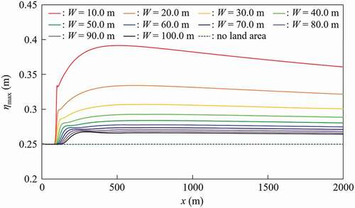
As depicted in Figure 7, when the river width W ≤ 80.0 m, the tsunami height distribution along the x-axis showed two peaks: the first peak at just upstream from the estuary, and the second peak located further upstream. The first peak was due to the superposition of the incident wave and diffracted wave, whereas the second peak was generated by the effect of the water surface curvature described above. When W = 10.0 m, the increase rate of tsunami height based on the incident wave height, i.e., r = (η – H₀)/H₀, was 33.7% for the first peak at x = 101.5 m, and 56.6% for the second peak at x = 508.5 m, whereas when W = 50.0 m, the increase rate r was 10.6% for the first peak at x = 178.5 m, and 13.6% for the second peak at x = 739.5 m. Therefore, as the increase rate of tsunami height, r, for the first peak was increased, the effect of the water surface curvature increased.

It should be noted that the second tsunami height peak at the river centerline was located more upstream as the river width was increased. As described for Figure 6, the wave height was distributed in the river crossing direction near the estuary, following which the wave height approached uniform in the river crossing direction as the tsunamis ascended the river. Therefore, as the river width was increased, the tsunami height required a longer distance, which was propagated by the tsunamis, to become uniform in the river crossing direction, so that the location of the second tsunami height peak at the river centerline occurred farer from the river mouth.

Conversely, when the river width W ≥ 90.0 m, the second tsunami height peak did not appear because the water surface curvature was not effective, and the tsunami height gradually decreased upstream from the first peak value, as indicated in Figure 7.

3.2. Tsunamis ascending a river with different still water depths

Figure 8 depicts the relative tsunami height η_max/H₀ along the x-axis indicated in Figure 3 in Case B. The solitary wave with wave height H₀ of 0.5 m was generated at x = 0.0 m. The still water depth h₀ was 2.5 m, 3.0 m, or 5.0 m everywhere in both the sea and river areas. The river width W was uniformly 20.0 m or 50.0 m. The figure indicates that as the river width W was decreased, the relative tsunami height η_max/H₀ increased everywhere in the river channels, for all the still water depths. The reason was that the diffracted wave energy was concentrated near the riverbank at the estuary, so that the diffracted wave energy per unit river width increased as the river width was decreased.

Figure 8. The distributions of the relative tsunami height η_max/H₀ along the x-axis indicated in Figure 3, for different still water depths h₀ and river widths W in Case B. The incident solitary wave height H₀ was 0.5 m.

Moreover, Figure 8 indicates that as the still water depth h₀ was increased, both the relative tsunami height η_max/H₀ in the river channels and the location x at which the maximum value of η_max/H₀ appeared increased, for both river widths. The representative wavelength λ of a solitary wave is defined by

(1) $\lambda =\underset{0}{\overset{50h_0}{\int }}\eta dx/H_0,$(1)

where η is water surface displacement, h₀ is still water depth, and H₀ is incident solitary wave height. Both the water surface displacements and water particle velocities of the incident waves adopted in this study were significant for a distance of less than 50h₀ in the wave propagation direction. From Equation (1)(1) $\lambda =\underset{0}{\overset{50h_0}{\int }}\eta dx/H_0,$(1) , when h₀ = 2.5 m, 3.0 m, and 5.0 m, the representative wavelengths λ for the solitary waves with wave height H₀ of 0.5 m are 13.8 m, 18.2 m, and 37.9 m, respectively. That is, for the incident solitary waves with the same wave height, the representative wavelength λ increases as the still water depth h₀ is increased. Therefore, as h₀ was increased, the wave energy diffracted to enter the river increased owing to the larger λ, so that the relative tsunami height η_max/H₀ increased in the river channel.

3.3. Tsunamis ascending a river with different riverbed gradients

The tsunamis ascending a river with uniform riverbed gradient β were simulated numerically in Case C, the conditions of which are described in Table 1. The side view of the calculation domain is illustrated in Figure 9, which is different from Figure 3(b), in which β = 0.0. The plan view of the calculation domain is the same as that depicted in Figure 3(a).

Figure 9. The side view of the calculation domain in Case C, the conditions of which are described in Table 1. The x-axis is along the centerline of the target river and β is the riverbed gradient.

Figure 10 depicts the distributions of the tsunami height η_max along the x-axis indicated in Figures 3(a) and 9, where tan β was 0.0, 5.0 × 10^–4, or 1.0 × 10^–3, and the river width W was 50.0 m. The solitary wave with wave height H₀ of 0.25 m was generated at x = 0.0 m, at which the still water depth h₀ was 2.5 m in the sea area. In the figure, the corresponding results without a land area are also depicted for different seabed gradients using the broken lines, where the still water depth was 2.5 m for 0.0 m ≤ x ≤ 100.0 m, and the seabed gradient was β for x > 100.0 m. Even when there is no land area, the tsunami height increased owing to the shallowing up to the wave breaking point at which the leading tsunami began to show the water surface fluctuation due to wave breaking. Figure 10 depicts the distributions of the tsunami height only offshore from the wave breaking points since this study’s main purpose is not to investigate the energy attenuation due to wave breaking. As the riverbed gradient β was increased, the tsunami height η_max increased at any location, with or without the land area. In the case without a land area, the wave breaking point was located at x ≃ 1035.5 m when tan β = 1.0 × 10^–3, whereas tsunamis did not show wave breaking when tan β = 5.0 × 10^–4. Conversely, supposing there is the land area, the tsunami height increased owing to not only the shallowing but also the effect of the water surface curvature after the tsunamis ran through the river mouth. When tan β = 1.0 × 10^–3, the tsunami height η_max increased sharply from x = 196.5 m to x = 706.5 m, approximately in proportion to x with a proportionality coefficient of 1.0 × 10^–4, following which the tsunami showed water surface fluctuation at x = 834.5 m, at which the still water depth was 1.77 m, and the tsunami height was 0.34 m. When tan β = 5.0 × 10^–4, the tsunami height showed the second peak at x = 1,312.5 m, and then the tsunami height decreased gradually until the tsunami showed water surface fluctuation at x = 1,375.5 m, at which the still water depth was 0.39 m.

Figure 10. The distributions of the tsunami height η_max along the x-axis indicated in Figures 3(a) and 9, for different riverbed gradients β in Case C. The solitary wave with wave height H₀ of 0.25 m was generated at x = 0.0 m, at which the still water depth h₀ was 2.5 m. The results for the tsunamis ascending the river with river width W of 50.0 m are depicted using the solid lines, whereas the corresponding results without a land area are depicted using the broken lines, where the still water depth was 2.5 m for 0.0 m ≤ x ≤ 100.0 m and the seabed gradient was β for x > 100.0 m.

3.4. Tsunamis ascending a river with different estuary shapes

The tsunamis ascending a river were simulated numerically when the coastline is diagonal to the river channel in Case D, the conditions of which are described in Table 1. The plan view of the calculation domain is depicted in Figure 11, which is different from Figure 3(a), considering the angle between the x-axis direction and coastline, namely the coastline angle θ_coast. The side view of the calculation domain was the same as that depicted in Figure 3(b).

Figure 11. The plan view of the calculation domain including a river channel in Case D, the conditions of which are described in Table 1. The gray region denotes a land area, the edges of which are vertical walls. The x-axis is along the centerline of the target river.

Figure 12 depicts the distributions of the tsunami height η_max along the x-axis indicated in Figures 3(b) and 11 in Case D, in which the coastline angle θ_coast was 45.0°, 60.0°, or 90.0°. The river width W was 20.0 m, the still water depth h₀ was 3.0 m, and the incident solitary wave height H₀ was 0.5 m. Based on Figure 12, the maximum increase rate of tsunami height based on the incident wave height, r_max, was 9.5%, 16.0%, and 31.1%, when θ_coast is 45.0°, 60.0°, and 90.0°, respectively. The tsunami height η_max in the river channels decreased, as the coastline angle θ_coast was decreased, because the diffracted waves were harder to enter the river channels when the coastline angle θ_coast is sharper.

Figure 12. The distributions of the tsunami height η_max along the x-axis indicated in Figures 3(b) and 11, for different coastline angles θ_coast in Case D. The river width W was 20.0 m, the still water depth h₀ was 3.0 m, and the incident solitary wave height H₀ was 0.5 m.

3.5. Tsunamis ascending a river narrowing toward the upstream

The tsunamis ascending a river were simulated numerically when the river width decreases linearly toward the upstream in Case E, the conditions of which are described in Table 1. The plan view of the calculation domain is depicted in Figure 13, which is different from Figure 3(a), considering the angle between the x-axis direction and riverbank line, namely the riverbank line angle θ_river. The side view of the calculation domain was the same as that depicted in Figure 3(b).

Figure 13. The plan view of the calculation domain including a river channel narrowing toward the upstream in Case E, the conditions of which are described in Table 1. The gray region denotes a land area, the edges of which are vertical walls. The x-axis is along the centerline of the target river.

Figure 14 depicts the distributions of the tsunami height η_max along the x-axis indicated in Figures 3(b) and 13 in Case E, in which the river width at the river mouth, W, was 100.0 m, and that at the upstream end, W', was 20.0 m; tan θ_river was 0.04. The still water depth h₀ was 3.0 m, and the incident solitary wave height H₀ was 0.5 m. The corresponding results for the rivers with uniform river widths of 20.0 m and 50.0 m are also depicted in Figure 14. At x = 512.5 m, the tsunami height η_max for the river narrowing toward the upstream was the same as that for the river with a uniform width of 50.0 m. At this location, the river’s width narrowing toward the upstream was 67.0 m, which was larger than 50.0 m. This means that the tsunami height can increase because of the contraction of the river width. The tsunami height in the narrowing river increased sharply from x = 423.5 m to x = 928.5 m, approximately in proportion to x with a proportionality coefficient of 1.25 × 10^–4, because both the river width contraction and water surface curvature were effective to increase the tsunami height. Thereafter, the tsunami showed water surface fluctuation at x ≃ 929.5 m, at which the river width was 33.6 m and the tsunami height was 0.62 m.

Figure 14. The distributions of the tsunami height η_max along the x-axis indicated in Figures 3(b) and 13 in Case E, in which the tangent of the riverbank line angle θ_river was 0.04. The river-mouth width W was 100.0 m, the still water depth h₀ was 3.0 m, and the incident solitary wave height H₀ was 0.5 m. The corresponding results are also depicted for the rivers with uniform river widths of 20.0 m and 50.0 m, where θ_river was 0.0°.

4. Tsunamis ascending a river for different incident wave conditions

4.1. Tsunamis ascending a river for different incident wave heights

The tsunamis ascending a river were simulated numerically for different incident wave heights in Case F, the conditions of which are described in Table 1. The calculation domain is depicted in Figure 3. Depicted in Figure 15 are the distributions of the relative tsunami height η_max/H₀ along the x-axis indicated in Figure 3, where the incident solitary wave heights H₀ were 0.25 m and 0.5 m. The river width W was of 20.0 m and 50.0 m, and the still water depth h₀ was 2.5 m. Figure 15 indicates that as the river width W was decreased, the relative tsunami height η_max/H₀ increased everywhere in the river channels for both incident solitary wave heights H₀. Conversely, as H₀ was decreased, both the relative tsunami height η_max/H₀ in the river channels and the location x at which the maximum value of η_max/H₀ appeared increased for both river widths W. When the still water depth h₀ is 2.5 m, the representative wavelengths λ defined by Equation (1)(1) $\lambda =\underset{0}{\overset{50h_0}{\int }}\eta dx/H_0,$(1) for the solitary waves with wave heights H₀ of 0.25 m and 0.5 m were 19.3 m and 13.8 m, respectively. Therefore, as the incident wave height H₀ was decreased, the representative wavelength λ of the incident solitary wave increased, so that the relative tsunami height η_max/H₀ increased in the river channels.

Figure 15. The distributions of the relative tsunami height η_max/H₀ along the x-axis indicated in Figure 3, for different incident solitary wave heights H₀ and river widths W in Case F, the conditions of which are described in Table 1. The still water depth h₀ was 2.5 m.

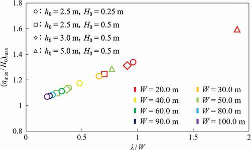
Figure 16 depicts the relationship between the maximum value of the relative tsunami height (η_max/H₀)_max and the ratio of representative wavelength to river width, λ/W, for 14 cases with different river widths W, still water depths h₀, and incident wave heights H₀. This figure indicates a positive correlation between (η_max/H₀)_max and λ/W for the present conditions. When λ/W < 1.0, (η_max/H₀)_max and λ/W were in a directly proportional relationship, which was approximately expressed by

(2) $({\eta }_{\mathrm{m}\mathrm{a}\mathrm{x}}/H_0{)}_{\mathrm{m}\mathrm{a}\mathrm{x}}=0.36\left(\lambda /W\right)+1.0\mathrm{w}\mathrm{h}\mathrm{e}\mathrm{n}\lambda /W<\mathrm{1.0.}$(2)

Figure 16. The relationship between the maximum value of the relative tsunami height, (η_max/H₀)_max, and the ratio of representative wavelength to river width, λ/W, for different river widths W, still water depths h₀, and incident solitary wave heights H_0.

4.2. Tsunamis ascending a river for different incident wave shapes

The tsunamis ascending a river were simulated numerically for different incident wave shapes in Case G, the conditions of which were described in Table 1. The calculation domain is illustrated in Figure 3, in which a solitary wave or bore-shaped wave with wave height H₀ of 0.25 m was generated at x = 0.0 m. The still water depth h₀ was 2.5 m, and the river width W was 50.0 m. The rise period, when the water level was raised at x = 0.0 m to create the bore-shaped wave without turbulence, was 90.0 s.

Figure 17 depicts the water surface profiles along the x-axis indicated in Figure 3, at t = 60.0 s, 120.0 s, and 180.0 s, for both the incident solitary and bore-shaped waves. The corresponding results in the region with no land area for the same incident bore-shaped wave are also depicted in Figure 17. In the absence of a land area, the bore-shaped wave propagated, keeping the wave height constant at the incident wave height of 0.25 m after the rise period. Conversely, when the bore-shaped wave travels into the river channel, the wave height increased as the bore-shaped wave propagated in the river, because diffracted waves generated near the estuary also entered the river channel while the high and long crest passed through the river mouth. When t = 180.0 s, the increase rate of tsunami height based on the incident wave height, r = (η_max – H₀)/H₀, at x = 500.0 m was 68.8%, which was much larger than the maximum increase rate r_max of 13.6% for the solitary wave with the same incident wave height H₀.

Figure 17. The time variation of the water surface profile along the x-axis indicated in Figure 3 in Case G, the conditions of which are described in Table 1. The river width W was 50.0 m, the still water depth h₀ was 2.5 m, and the incident wave height H₀ was 0.25 m. The black solid lines depict the results for the bore-shaped wave, whereas the gray solid lines for the solitary wave with the same incident wave height. The corresponding results for the bore-shaped wave traveling in the region with no land area are also depicted with the broken lines.

Figure 17 also indicates that as the bore-shaped wave ran up the river, the water surface gradient at the front of the wave increased, because the wave nonlinearity was more effective than the wave dispersion.

5. Tsunamis ascending a river with a compound cross-section

The tsunamis ascending a river with a compound cross-section were simulated numerically. Figure 18 illustrates the calculation domain, in which the still water depth was uniformly 3.0 m in the main channel, whereas 0.5 m in the flood channels. The width of the target river, including the flood channels on both the left and right bank sides, was 200.0 m, and that of the target main channel was 100.0 m. The conditions for the calculation in Section 5 are summarized in Table 2.

Figure 18. The plan view of the calculation domain and the compound cross-section of the river in Case H, the conditions of which are described in Table 2. The gray regions denote land areas, the edges of which are vertical walls. The x-axis is along the centerline of the target river, and the y-axis is across the river.

The time variations of the water surface profile and velocity vectors in the cross-section at x = 600.0 m are presented in Figure 19, where the solitary wave with wave height H₀ of 0.5 m was generated at x = 0.0 m. In the flood channel, the first peak approached the riverbank because it had a wave component propagating across the river. Therefore, a high water level appeared at the riverbank based on the wave reflection at t = 135.0 s. The first wave reflected on the riverbank superposed the second wave from the main channel when t = 140.0 s. When t = 155.0 s, the tsunami propagated in the flood channel, showing a re-reflection between the flood plain and main channel, which means that part of the tsunami energy was trapped in the flood channel.

Figure 19. The time variations of the water surface profile and velocity vectors in the cross-section at x = 600.0 m, when the tsunamis ascend the river with the compound cross-section depicted in Figure 18. The incident solitary wave height H₀ was 0.5 m.

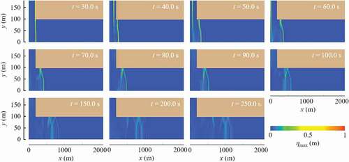
Figure 20 depicts the time variation of the water level distribution in the same case. The phase velocity in the flood channel was slower than that in the deeper main channel. Because this led to the phase velocity distribution in the river crossing direction, the wave direction was diagonal to the river centerline and the crest line was stretched in the flood channel. This effect, together with wave breaking, caused the tsunami height to be lower than the incident wave height in the flood channel, except at the riverbank. It should be noted that multiple crest lines appeared in both the main and flood channels because of the reflections of the tsunamis traveling diagonally to the river channel, although the single cross-section river with the same width as the main channel's width of the compound cross-section river, namely 100.0 m, did not generate wave disintegration, as described for Figure 7.

Figure 20. The time variation of the water level distribution, when the tsunamis ascend the river with the compound cross-section depicted in Figure 18. The incident solitary wave height H₀ was 0.5 m.

6. Conclusions and recommended countermeasures against river tsunamis

The three-dimensional numerical simulations were generated for different river topographies and incident waves to investigate the fundamental characteristics of tsunamis ascending a river. First, we examined the tsunamis running up the single cross-section rivers with different topographies when a solitary wave is incident. The tsunami height, defined as the maximum water level at each location, increased in the vicinity of the riverbank at the estuary because the diffracted wave also entered the river channel. Therefore, as a countermeasure against tsunamis that run up a river, it is necessary to install an embankment near the river mouth considering the water level rise as shown in the calculation results, because conventional riverbanks are designed for the flows from the upstream to downstream, and the riverbanks near a widened estuary are not designed to be so high and strong, even against storm surges and high wind waves.

After the diffracted waves that entered the rivers caused the wave height distribution in the river crossing direction near the river mouth, the wave height gradually became uniform in the river crossing direction as the tsunamis ran up the river, and then became larger than the incident wave height, even at the river centerline.

Moreover, as the tsunamis propagated in the narrow rivers, the radius of the water surface curvature around the first peak of the water surface profile decreased, increasing the tsunami height with wave disintegration until the appearance of the second tsunami height peak. The location of the second tsunami height peak was farer from the river mouth as the uniform river width was wider. Therefore, the riverbank height, flood area, ship mooring, evacuation preparation, etc. should be designed, considering the risk that the tsunami height will increase upstream.

When the tsunamis ascend the rivers that are shallower or narrower upstream, the tsunami height increased based on the shallowing and energy concentration, until the tsunamis showed the water surface fluctuation due to wave breaking. As the angle between the riverbank line and coastline at the estuary was decreased, the tsunami height decreased everywhere in the river, because the diffracted waves were harder to enter the river when the angle is sharper. Therefore, to prevent the incident of diffracted waves at an estuary, the angle between a riverbank line and coastline is desirable to be an acute angle.

Second, the tsunamis ascending the rivers were examined for different incident wave conditions. The tsunami height increased in the rivers, depending on not only the incident wave height but also the ratio of representative wavelength to river width. As this ratio was increased, the tsunami height in the rivers increased, which suggests that when a tsunami retains a long wavelength without much wave disintegration offshore and enters a river, the risk posed by the river tsunami will increase.

Moreover, when the bore-shaped wave travels into the river, the maximum tsunami height was larger than that of the solitary wave with the same incident wave height. This means that even when the wave height is similar for multiple tsunamis that enter a river, the tsunami height can become different in the river, depending on the wave shapes.

Finally, in the case determining the tsunamis running up the river with the compound cross-section, the tsunamis traveled diagonally in the flood channel and showed multiple reflections both on the riverbank and between the flood and main channels, leading to the multiple crestlines. For the present conditions, the tsunami height was lower in the flood channel than the incident wave height, except at the riverbank, owing to both the wave breaking and diagonally traveling of the tsunamis. At a riverbank, the water level will rise based on wave reflection, as indicated by the calculation result, so that it is important to note that tsunamis can cross a low riverbank even when the tsunami height inside a flood channel is not so large.

Future work is required to study the effects of wave breaking, riverbed friction, vegetation, etc. on tsunamis ascending rivers, considering more complicated river topographies, including river curvature and tributaries, using three-dimensional models.

Acknowledgments

Sincere gratitude is extended to two anonymous reviewers for their precious comments that improved the clarity of the manuscript and enriched the interpretation of the results.

Disclosure statement

No potential conflict of interest was reported by the authors.

References

- Arikawa, T., H. Yamada, and M. Akiyama. 2005. “Examination of Applicability of Tsunami Wave Force in Three-dimensional Numerical Wave Tank.” Annual Journal of Coastal Engineering, JSCE 52: 46–50. doi:https://doi.org/10.2208/proce1989.52.46. (in Japanese).
- Bricker, J. D., S. Gibson, H. Takagi, and F. Imamura. 2015. “On the Need for Larger Manning’s Roughness Coefficients in Depth-integrated Tsunami Inundation Models.” Coastal Engineering Journal 57 (2) Article ID 1550005: 13 pages. doi:https://doi.org/10.1142/S0578563415500059.
- Coastal Development Institute of Technology. 2010. “CADMAS-SURF/3D Research and Development of Numerical Wave Tank.” CDIT Library 39: 235p. ISBN:9784900302860. (in Japanese).
- Esteban, M., J. J. Roubos, K. Iimura, J. T. Salet, B. Hofland, J. Bricker, H. Ishii, G. Hamano, T. Takabatake, and T. Shibayama. 2020. “Effect of Bed Roughness on Tsunami Bore Propagation and Overtopping.” Coastal Engineering 157 Article ID 103539: 11 pages. doi:https://doi.org/10.1016/j.coastaleng.2019.103539.
- Fritz, H. M., C. M. Petroff, P. Catalán, R. Cienfuegos, P. Winckler, N. Kalligeris, R. Weiss, S. E. Barrientos, G. Meneses, C. Valderas-Bermejo, C. Ebeling, A. Papadopoulos, M. Contreras, R. Almar, J. C. Dominguez, and C. E. Synolakis. 2011. “Field Survey of the 27 February 2010 Chile Tsunami.” Pure and Applied Geophysics 168 (11): 1989–2010. doi:https://doi.org/10.1007/s00024-011-0283-5.
- Fujima, K., C. Goto, and N. Shuto. 1984. “Numerical Study on Nonlinear Dispersion Wave Theory.” Annual Journal of Coastal Engineering, JSCE 31: 93–97. doi:https://doi.org/10.2208/proce1970.31.93. (in Japanese).
- Iwasaki, T., T. Abe, and K. Hashimoto. 1977. “Study on the Characteristic of River Tsunami.” Proceedings of the 24th Japanese Conference on Coastal Engineering, JSCE: 74–77. doi:https://doi.org/10.2208/proce1970.24.74. (in Japanese).
- Kakinuma, T., G. Tsujimoto, T. Yasuda, and T. Tamada. 2012. “Trace Survey of the 2011 Tohoku Tsunami in the North of Miyagi Prefecture and Numerical Simulation of Bidirectional Tsunamis in Utatsusaki Peninsula.” Coastal Engineering Journal 54 (1) Article ID 125007: 28 pages. doi:https://doi.org/10.1142/S0578563412500076.
- Kalmbacher, K. D., and D. F. Hill. 2015. “Effects of Tides and Currents on Tsunami Propagation in Large Rivers: Columbia River, United States.” J. Waterway, Port, Coastal, and Ocean Engineering 141 (5) Article ID 04014046: 8 pages. doi:https://doi.org/10.1061/(ASCE)WW.1943-5460.0000290.
- Kayane, K., M. Roh, H. Tanaka, and X. T. Nguyen. 2011. “Influence of River Mouth Topography and Tidal Variation on Tsunami Propagation into Rivers.” Journal of JSCE, Ser. B2 (Coastal Engineering) 67 (2): I_246–I_250. doi:https://doi.org/10.2208/kaigan.67.I_246. (in Japanese).
- Longuet-Higgins, M. S., and J. D. Fenton. 1974. “On the Mass, Momentum, Energy and Circulation of a Solitary Wave II.” Proceedings of the Royal Society of London, Ser. A 340: 471–493. doi:https://doi.org/10.1098/rspa.1974.0166.
- Murashima, Y., S. Koshimura, H. Oka, Y. Murata, T. Suzuki, and F. Imamura. 2010. “Numerical Simulation of Tsunami Run-up on Tokachi River Using Nonlinear Dispersive Wave Equations Model and Evaluation of Space Grid Size.” Journal of JSCE, Ser. B2 (Coastal Engineering) 66 (1): 206–210. doi:https://doi.org/10.2208/kaigan.66.206. (in Japanese).
- Nakamura, Y., T. Kakinuma, and T. Asano. 2017. “A Numerical Simulation for the Tsunami Ascending Rivers.” Journal of JSCE, Ser. B2 (Coastal Engineering) 73 (2): I_331–I_336. doi:https://doi.org/10.2208/kaigan.73.i_331. (in Japanese).
- River Tsunami Countermeasures Study Group. 2011. “Urgent Recommendations on River Run-up Tsunami Counter-measures.” Ministry of Land, Infrastructure, Transport and Tourism, Japan: 10p. Accessed 17 November 2021. http://www.mlit.go.jp/common/000163992.pdf .
- Shuto, N. 1985. “The Nihonkai-Chubu Earthquake Tsunami on the North Akita Coast.” Coastal Engineering in Japan 28 (1): 255–264. doi:https://doi.org/10.1080/05785634.1985.11924420.
- State of Oregon Department of Geology and Mineral Industries. 2021. “Oregon Tsunami Clearinghouse.” Accessed 17 November 2021. https://www.oregongeology.org/tsuclearinghouse .
- Sun, J. S., O. W. H. Wai, K. T. Chau, and R. H. C. Wong. 2009. “Prediction of Tsunami Propagation in the Pearl River Estuary.” Science of Tsunami Hazards, International Journal of the Tsunami Society 28: 142–153. ISSN:.
- Tanaka, H., K. Ishino, B. Nawarathna, H. Nakagawa, S. Yano, H. Yasuda, Y. Watanabe, and K. Hasegawa. 2008. “Field Investigation of Disasters in Sri Lankan Rivers Caused by the 2004 Indian Ocean Tsunami.” Journal of Hydroscience and Hydraulic Engineering 26: 91–112.
- Tanaka, H., N. X. Tinh, N. T. Hiep, K. Kayane, M. Roh, M. Umeda, M. Sasaki, S. Kawagoe, and M. Tsuchiya. 2020. “Intrusion Distance and Flow Discharge in Rivers during the 2011 Tohoku Tsunami.” Journal of Marine Science and Engineering 8 (11) Article ID 882: 12 pages. doi:https://doi.org/10.3390/jmse8110882.
- Tanimoto, K., N. Tanaka, N. B. Thuy, and K. Iimura. 2008. “Effect of Coastal and River Forests on Tsunami Run-up in River.” Annual Journal of Coastal Engineering, JSCE 55: 226–230. doi:https://doi.org/10.2208/proce1989.55.226. (in Japanese).
- Tolkova, E., and H. Tanaka. 2016. “Tsunami Bores in Kitakami River.” Pure and Applied Geophysics 173 (12): 4039–4054. doi:https://doi.org/10.1007/s00024-016-1351-7.
- Tsuji, Y., T. Yanuma, I. Murata, and C. Fujiwara. 1991. “Tsunami Ascending in Rivers as an Undular Bore.” Natural Hazards 4: 257–266. doi:https://doi.org/10.1007/BF00162791.
- Viana-Baptista, M. A., P. M. Soares, J. M. Miranda, and J. F. Luis. 2006. “Tsunami Propagation along Tagus Estuary (Lisbon, Portugal) Preliminary Results.” Science of Tsunami Hazards, International Journal of the Tsunami Society 24 (5): 329–338. ISSN:.
- Yasuda, H. 2010. “One-dimensional Study on Propagation of Tsunami Wave in River Channels.” Journal of Hydraulic Engineering 136 (2): 93–105. doi:https://doi.org/10.1061/(ASCE)HY.1943-7900.0000150.
- Yeh, H., E. Tolkova, D. Jay, S. Talke, and H. Fritz. 2011. “Tsunami Hydrodynamics in the Columbia River.” Journal of Disaster Research 7 (5): 604–608. doi:https://doi.org/10.20965/jdr.2012.p0604.