Validation of tsunami numerical simulation models for an idealized coastal industrial site

ABSTRACT

Numerous tsunami numerical models have been proposed, but their prediction accuracies have not been directly compared. For quantifying the modeling uncertainties, the authors statistically analyzed the prediction results submitted by participants in the tsunami blind contest held at the 17th World Conference on Earthquake Engineering. The reproducibility of offshore water level generated due to the tsunami with soliton fission significantly decreased when the nonlinear shallow water equation models (NSWE) was used compared to three-dimensional (3D) models. The inundation depth was reproduced well in 3D models. However, the reproducibility of wave forces acting on the structure and velocities over land was lower in 3D models than that in NSWE models. For cases where the impulsive tsunami wave pressure generated could not be calculated based on the hydrostatic assumption, the prediction accuracy of the NSWE models was higher than that of the 3D models. The prediction accuracies of both models were not improved at small grid-cell sizes. The NSWE model cannot simulate the short-wave component and vertical pressure distribution. Therefore, further developments in 3D models and smoothed particle hydrodynamics methods (SPH) are needed. The presented results contribute to the future development of tsunami numerical simulation tools.

KEYWORDS:

• Tsunami
• numerical simulation
• laboratory test
• validation

1. Introduction

Tsunamis are long waves triggered by submarine earthquakes, landslides, volcanoes activity, and the impact of extraterrestrial objects. More than 2600 tsunamis have been recorded since 2000 BCE in the Atlantic, Indian, and Pacific oceans, and the Caribbean and Mediterranean seas. Among them, more than 2000 tsunamis were triggered by earthquakes, volcano-tectonic earthquakes, earthquake-induced landslides, and combinations of these three processes. Tsunamis cause numerous casualties and various damages to buildings. Indeed, (Sugawara etal. 2020) the death toll reached 20,416 (including missing people) due to the 2011 Great East Japan Tsunami, which was triggered by a 9.0 magnitude (Mw) undersea megathrust earthquake (Arikawa et al. 2012).

The mechanisms behind tsunami generation are generally understood, but the prediction of its propagation and inundation remains a formidable challenge due to the complexities of coastline formations and the presence of numerous coastal structures that interact and alter the flow (Rogers and Dalrymple 2008). Numerical simulations have been conducted to estimate the coastal inundation due to tsunamis and its induced damages (e.g. Marras and Mandli 2021). The nonlinear shallow water equation (NSWE) model is a useful tool for simulating the propagation of long tsunami waves in deep oceans. The NSWE model is computationally efficient; thus, it is effective for large domain simulations during wave propagation (Xie, Nistor, and Murty 2012). However, the NSWE model cannot consider the dispersion effects during tsunami propagation and simulate the bores or soliton fissions. To account this, nonlinear dispersive wave models (hereinafter, Boussinesq models) have been proposed. Indeed, some open-source codes of Boussinesq models, such as the fully nonlinear Boussinesq wave model with Total Variation Diminishing (FUNWAVE-TVD) (Shi et al. 2012) and the Cornell University Long and Intermediate Wave Modeling (COULWAVE) (Lynett et al. 2002), have been distributed. However, the NSWE model or Boussinesq model cannot calculate the vertical distribution of the flow. Although three-dimensional (3D) multilayer hydrostatic models (Pietrzak et al. 2002) have been developed, the hydrostatic pressure assumption is not valid for short surface waves and stratifications induced by strong density gradients. Therefore, non-hydrostatic multilayer models (Kocyigit et al. 2002; Abualtayef et al. 2008; Ai and Jin 2008, 2012) have also been developed.

Recently, three-dimensional models have been used (Choi et al. 2008; Wijatmiko and Murakami 2010) for tsunami simulation. Open-source codes, such as the Open-FOAM (Higuera, Lara, and Losada 2013) and SUper Roller Flume for Computer Aided Design of MAritime Structure in 3D (CADMAS-SURF3D), are available (Arikawa, Yamano, and Akiyama 2007). However, for three-dimensional simulation, the free surface must be defined using the Volume of Fluid (VOF) method (Hirt and Nichols 1981). In tsunami simulations based on the smoothed particle hydrodynamics (SPH) methods (Rogers and Dalrymple 2008; Sarfaraz and Pak 2017), wave breaking, and other flows that result in fluid separation are modeled as quickly as other flows (Rogers and Dalrymple 2008). In the SPH technique, fixed computational grids are not required when calculating spatial derivatives, making it suitable for solving the tsunami–structure interactions (Huang and Zhu 2015). Owing to its simplicity and robustness, the SPH has been extended to study dynamic phenomena in solid mechanics for dynamic phenomena and, more recently, to complex fluid mechanics problems such as dam-break and wave propagation (Xie, Nistor, and Murty 2012). The moving particle simulation (MPS), a pure Lagrangian mesh-less method initially developed by Koshizuka and Oka (1996) for the fragmentation of incompressible fluids can track free surfaces with large deformations. The method has been applied in various engineering fields (Huang and Zhu 2015).

Several tsunami benchmark problems have been provided for the validation or verification of numerical simulation model (e.g. Synolakis et al., 2007). Although the assessments of numerical simulation models have been conducted (e.g. Watts, Imamura, and Grilli 2011; Macías, Castro, and Sánchez 2020), the accuracies of the proposed models have not been directly compared. For improving the evaluation technologies of tsunami simulation models, it is essential to understand the proposed approaches, the determination of modeling parameters, and the accuracy of current analytical approaches. Moreover, investigating the variability of the numerical simulations is also important for predicting the damage situation using the tsunami fragility function (Koshimura et al. 2002; Mas et al. 2012; Suppasri, Koshimura, and Imamura 2011; Suppasri et al. 2012).

To address the above-mentioned problems, a tsunami blind contest (Arikawa et al. 2021) was held at the 17th World Conference on Earthquake Engineering (17WCEE) at Sendai City, Japan, from September 27 to October 2 2021(International Association for Earthquake Engineering undated). A set of hydraulic experiments was conducted (Kihara et al. 2021), in which a tsunami wave was passed a seaside area where several buildings and tanks were installed. The tsunami wave pressure acting on buildings and tanks, water depths, and velocities were measured (Kihara et al. 2021). The contestants were asked to predict these values, and the prediction accuracies were quantified. The results of the laboratory experiments were not available to the contestants. Thus, the accuracy of the tsunami numerical simulation models was investigated without setting the parameter that adjusted the experimental. For conducting the numerical simulation, many settings, such as simulation models, turbulent models, and resolutions of grid-cell sizes, are necessary to be determined. Owing to these selections, the simulation results are likely to be varied. The main objective in analyzing the results of the tsunami blind contest was to reveal these uncertainties

In this study, the authors summarized the prediction results calculated by the blind contest participants. The authors then evaluated the accuracy of the results calculated using various numerical tsunami simulation models. The evaluation results are helpful for the future development of a high precision numerical simulation model for tsunami inundation. It will provide important information for risk-informed and performance-based engineering.

2. Method

2.1. Laboratory experiment

The objective of the experiment was to evaluate the tsunami inundation in a seaside area and the wave pressures acting on the buildings and tanks installed in the area. The experiment was conducted using the large wave flume of the Central Research Institute of Electric Power Industry, Japan. A brief description of the experiment is provided here, and the details of the experiments can also be found in Kihara et al. (2021). The flume was 205 m long, 3.4 m wide, and 6.0 m deep open channel, made of reinforced concrete. A piston-type wave generator with a steel paddle and dry-back design was installed at the offshore side of the flume. The maximum stroke of the piston was 2.2 m, and the positions of the steel paddle were connected to a computer and can be controlled by the user. A tsunami-like wave was generated by the wave generator offshore, which then inundated the seaside area. The elevation view of the experimental setup is shown in Figure 1, along with the coordinate system. The x, y, and z axes denote the streamwise, transverse, and vertical directions. The origin of the coordinate system was set at the intersection of the shoreline, the concrete bed of the seaside area, and the right bank of the flume. The bed profiles of the flume consisted of a horizontal section near the wave generator at x < −79.25 m, a 1/10.36 sloped section at −79.25 m < x < −41.33 m, a 1/226.24 sloped section at −41.33 m < x < 0 m and 25.0 < x < 73.863 m, and a 1/15 sloped section at x > 73.863 m. At 0 m < x < 25.0 m, a seaside area with a horizontal flatbed was installed on the 1/215 sloped section. The bed of the seaside area was made of wood panels with a surface coating to ensure a smooth surface. The seaside area was modeled as an idealized seaside industrial site with a scale of 1/50 based on the Froude similarity. Several models of buildings and tanks were then installed on the seaside area in the form of acrylic cuboids and cylinders, respectively. The positions, dimensions, and photographs of the buildings and tank models are shown in Figures 2–4, respectively. Figure 2 illustrates the x and y coordinates of the upstream-right bank corners of the building models and the center of the tank models. Eight wire resistance wave gauges (WG) were installed at the coordinates (Table 1) and were used to collect the measurements for each experiment. In this series of experiments, separate experiments were conducted to measure pressure, inundation depth, and velocity at the seaside area because the measurements of inundation depth and velocity disturb the inundation flows due to the use of contact-type instruments. Pressures were measured at different heights along several vertical lines on the buildings and tanks identified as P1, P2, P3, P4, and P5 in Figure 2. The locations of the lines are shown in Figure 5. Pressures were measured at eight elevations, that is, z = 0.01, 0.025, 0.05, 0.075, 0.10, 0.15, 0.21, and 0.27 m along the lines at the red points, and at six elevations, that is, z = 0.01, 0.05, 0.10, 0.15, 0.20, and 0.245 m along the lines at the green points. The pressure was simultaneously measured along five measurement lines using 32 pressure transducers (SSK Co., Ltd., p306; upper-pressure limit of 0.98 kPa). Inundation depths and velocities were measured at 14 locations aligned in a 7 × 2 grid, as shown in Figure 6. The inundation depth was measured simultaneously at two points with the same x-coordinates; the experiments were repeated under the same tsunami conditions at least twice for each pair of measurement points. The velocity at z = 0.015 m was also measured at least twice for each x-coordinate pair using two electromagnetic velocimeters under the same tsunami conditions.

Figure 1. Elevation view of the experimental set up. Coordinates (x, z) of key positions are shown (Arikawa et al. 2021).

Figure 2. Positions of building and tank models in the seaside area. x and y coordinates are shown for the upstream-right bank corners of the building models and for the centers of the tank models. The dashed lines in the figure are straight lines parallel to the x and y axes indicating the positions of the small cubic building models (Arikawa et al. 2021).

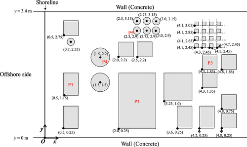
Figure 3. Dimensions of the building and tank models (Arikawa et al. 2021).

Figure 4. Photographs of building and tank models in the seaside area (Arikawa et al. 2021).

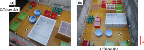
Figure 5. Locations of pressure-measurement lines on the building and tank models (Arikawa et al. 2021).

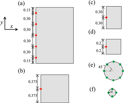
Figure 6. Locations of inundation depth and velocity measurements in the seaside area (red dots) (Arikawa et al. 2021).

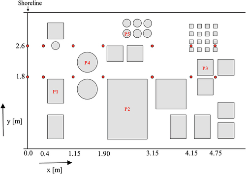
Table 1. Positions of the wave gage (WG) measurement points in the experimental set up (Arikawa et al. 2021)

Measurement points	x [m]	y [m]
WG1	−91.88	1.70
WG2	−78.52	1.70
WG3	−41.54	1.70
WG4	−30.00	1.70
WG5	−20.00	1.70
WG6	−10.00	1.70
WG7	−5.00	1.70
WG8	0.00	1.70

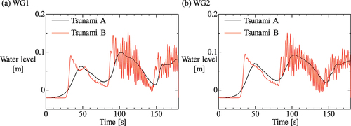
The pressures were recorded using a data logger (Kyowa Electronic Instruments Co., Ltd., EDX-3000A) at a sampling rate of 1 kHz. The water levels, inundation depths, and velocities were recorded in a second data logger (Keyence, NR-600) with a sampling rate of 100 Hz. Synchronization between the two data loggers and different experiments under the same tsunami conditions was obtained using electric signals. The experiments were conducted under two tsunami conditions, tsunamis A and B. The time series of the water levels at WG1 and WG2 are shown in Figure 7.

Figure 7. Time-series of the water levels at (a) WG1 and (b) WG2 for tsunamis A and B (Arikawa et al. 2021).

2.2. The collected data

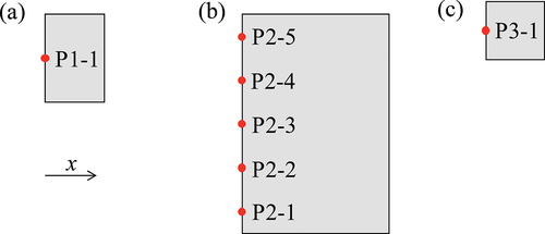
Contestants were requested to evaluate the time series and estimate the maximum values of velocities, water levels, inundation depths, and pressures on buildings and tanks under tsunami conditions A and B, either analytically or numerically. The time series of the water levels at WG1 and WG2 for both tsunami conditions were provided for setting tsunami conditions in the analytical models. The water levels were maximum at WG3-WG8 between 0 s and < 100 s. The inundation depths were maximum at y = 1.8 and 2.6 m and x = 0.0–4.75 m between 0 s and < 100 s. Velocities were estimated in the x-direction when the maximum inundation depths were observed at 0 s < time < 100 s at y = 1.8 and 2.6 m and x = 0.0–4.75 m. Pressures on the building models P1, P2, and P3 were estimated at the upstream face of the models when their vertically integrated values reached a maximum at 0 s < time < 100 s. The positions of the pressure measurements are shown in Figure 8. The following integral method was used for the vertical integration of pressures.

Figure 8. Positions of pressure measurement lines requested as the submission for building models (a) P1, (b) P2, and (c) P3 (Arikawa et al. 2021).

(1) $F=p_1\mathrm{\Delta }{z}_1+\frac{1}{2}\left(p_1+p_2\right)\mathrm{\Delta }{z}_2+\frac{1}{2}\left(p_2+p_3\right)\mathrm{\Delta }{z}_3+\dots +\frac{1}{2}\left(p_{n-1}+p_n\right)\mathrm{\Delta }{z}_n$(1)

where F is the vertically integrated value; $p_k\left(k=1,2,\dots ,n\right)$ is pressure; $\mathrm{\Delta }{z}_k\left(k=1,2,\dots ,n\right)$ is the distance between the pressure measurement height; $n$ is the number of measurement heights in a vertical line, and the schematic diagram of the integration is shown in Figure 9. The pressures on the tank models P4 and P5 were estimated at several vertical lines, whose positions are shown in Figure 10. For the tank models, pressures were estimated when the difference of vertically integrated values between the upstream and downstream lines became maximum at 0 s < time < 100 s.

Figure 9. A schematic diagram of pressure integration (Arikawa et al. 2021).

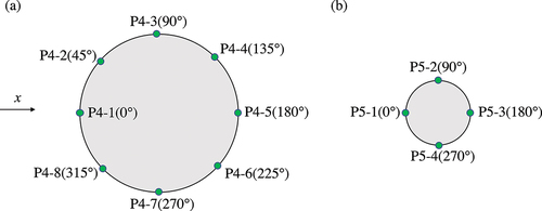
Figure 10. Positions of pressure measurement lines requested as the submission for tank models (a) P4 and (b) P5 (Arikawa et al. 2021).

Statistically averaged data were used for the test. Although water levels, inundation depths, and velocities were logged with a sampling rate of 100 Hz, data averaged by the “simple moving average” method with a 0.1 s period were used. In the case of pressures, which were logged with a sampling rate of 1000 Hz, data averaged by the simple moving average method with a 0.01 s period were used. For example, the averaged value $\bar{\eta }$ with a 0.1 s period is calculated as

(2) $\bar{\eta }\left(t\right)=\frac{1}{0.1}\underset{t}{\overset{t+0.1}{\int }}\eta \left(t{ }^{\mathrm{\prime }}\right)dt{ }^{\mathrm{\prime }}=\frac{1}{10}\sum _t^{10}\eta \left(t{ }^{\mathrm{\prime }}\right)$(2)

where $\eta$ is the logged value with a sampling rate of 100 Hz.

2.3. The methods of numerical simulation conducted by each participant

Fourteen participants (six individuals, six teams, and two anonymous participants) attended the blind contest and submitted the prediction results (see Supplementary Material 1). The submitted simulation results were calculated using seven types of numerical models. Some participants submitted more than one case and used the same type of numerical simulation models. Therefore, there were a total of 38 simulated results. Amongst them, nine were two-dimensional models (8 NSWE models and 1 Boussinesq model) meaning that there is no vertical layer, and the other 29 were three-dimensional models (non-hydrostatic incompressible fluid dynamics model, non-hydrostatic compressible fluid dynamics model, SPH, three-dimensional and non-hydrostatic model, three-dimensional and multilayer hydrostatic model). Amongst the 38 simulated results, 23 were non-hydrostatic incompressible fluid dynamics models, 1 a non-hydrostatic compressible fluid dynamics model (both hereinafter referred to as 3D models), 8 NSWE models, 3 SPH methods, 1 three-dimensional and non-hydrostatic model (hereinafter, 3D-NH model), 1 three-dimensional and multilayer hydrostatic model (hereinafter, 3D-H model), and 1 Boussinesq model (Table 2). The numerical simulation models used by the participants are shown in Table 3. For the NSWE model, the participants used their own proposed models.

Table 3. The numerical simulation models used by the participants

Model name	Reference
STOC-ML	Tomita et al. (2005)
STOC-IC	Tomita and Kakinuma (2005)
Open-FOAM	Weller et al. (1998)
FLOW-3D	Flow Science. (undated)
Advance/FrontFlow/red	AdvanceSoft. (undated)

Table 2. All conditions of numerical simulations submitted by the 14 participants

Analytical approach	Nonhydrostatic incompressible fluid dynamics model	Nonhydrostatic compressible fluid dynamics model	Nonlinear shallow water equation model	SPH	Three-dimensional and non-hydrostatic model	Three-dimensional and multilayer hydrostatic model	Nonlinear dispersive wave model
Number of results	23	1	8	3	1	1	1
Resolution (m) (x, y, z)	0.006–0.10, 0.006–0.10, 0.005–0.25	0.006–0.10, 0.006–0.10, 0.005–0.25	0.005–0.05, 0.005–0.05	Particle diameter; 0.01–0.06 m	0.02, 0.02, 0.05–0.15	0.02, 0.02, 0.05–0.15	0.02, 0.02
Turbulence model	Laminar, LES (Smagorinsky model, dynamic k equation model), RANS (k-ε model, k-ω model)	LES (Smagorinsky model)	-	Eddy viscosity model	-	-	-
Free surface	VOF method	VOF method	-	-	-	-	-
Wall boundary	Velocity; Spalding formula, Neumann condition, No SlipPressure; Neumann condition, Dirichlet condition, Fixed Flux	Velocity;No SlipPressure;Fixed Flux	-	Fixed wall ghost particle (FWGP) approach	-	-	-
Roughness	-	-	Manning’s roughness coefficient (0.009–0.015 s/m^1/3)	-	-	-	Manning’s roughness coefficient (land: 0.01 s/m^1/3, offhore: 0.01 s/m^1/3)
Method to calculate wave pressure	-	-	Arimitsu, Ooe, and Kawasaki (2012)	-	-	-	Arimitsu, Ooe, and Kawasaki (2012)

The range of grid-cell size (particle diameter in case of SPH) at the wave tank used in these simulations is shown in Table 2. Uniform grid-cell sizes were used in NSWE models. The grid-cell sizes were varied in the range 0.005–0.05 m in x and y directions. The turbulence models and the wall boundary conditions for velocity and pressure used in the numerical models are shown in Table 2.

For the NSWE model, the wave pressure cannot be calculated directly. Hence, the participants who adopted the NSWE model used the equation proposed by Arimitsu (2012) for the wave pressure calculations (Equation 3(3) $P_{max}\left(z\right)=\left\{\begin{array}{c}\rho g\left(h_{fmax}-z\right);z>h_{ufmax}\\ \rho g\left(h_{fmax}-z\right)+\rho u_{fmax}^2;z\le h_{ufmax}\end{array}\right.$(3) ).

(3) $P_{max}\left(z\right)=\left\{\begin{array}{c}\rho g\left(h_{fmax}-z\right);z>h_{ufmax}\\ \rho g\left(h_{fmax}-z\right)+\rho u_{fmax}^2;z\le h_{ufmax}\end{array}\right.$(3)

where $P_{max}\left(z\right)$ is the maximum pressure on the buildings; $\rho$ is the density of the fluid; g is the acceleration due to gravity; z is the distance from the bed; $h_{fmax}$ is the maximum inundation depth on the building; $u_{fmax}$ is the maximum velocity on the building; $h_{ufmax}$ is the inundation depth on the building when the maximum velocity is generated.

In the nonlinear dispersive wave model simulation, the wave pressure was calculated using Equation (3)(3) $P_{max}\left(z\right)=\left\{\begin{array}{c}\rho g\left(h_{fmax}-z\right);z>h_{ufmax}\\ \rho g\left(h_{fmax}-z\right)+\rho u_{fmax}^2;z\le h_{ufmax}\end{array}\right.$(3) . Some participants used turbulence models as 3D models. The turbulence models used by the participants were based on the Large Eddy Simulation (LES) and Reynolds Averaged Navier-Stokes (RANS) models. Participants used Smagorinsky model (Smagorinsky 1963) and dynamic k equation model (Kim and Menon 1995) in LES and k-ε model (Launder and Spalding 1974) and k-ω model (Wilco 2006) in RANS.

Participants who used the SPH model adopted the dynamic eddy viscosity model as the turbulence model. The other models did not use turbulence models.

2.4. Evaluation of prediction results

The participants computed the time series of tsunami water level at WG3-WG6, inundation depth and velocity at y = 1.8 m and y = 2.6 m, and wave pressure at P1-1, P2-1 – P2-5, P3-1, P4-1 – P4-8, and P5-1 – P5-4 for tsunamis A and B. The participants also computed the maximum tsunami water level, inundation depth, velocity, and wave pressure at the same points by calculating the ratio of calculation results/observation results at all observation points. The authors converted the pressure to wave force based on Equation (1)(1) $F=p_1\mathrm{\Delta }{z}_1+\frac{1}{2}\left(p_1+p_2\right)\mathrm{\Delta }{z}_2+\frac{1}{2}\left(p_2+p_3\right)\mathrm{\Delta }{z}_3+\dots +\frac{1}{2}\left(p_{n-1}+p_n\right)\mathrm{\Delta }{z}_n$(1) and then compared the calculated and observed wave forces. The model’s performance cannot be evaluated using results with low prediction accuracy. Therefore, to assess the model performance, the authors selected the submitted results based on prediction accuracy. The authors selected 28 of the 38 cases of the simulation results (Table 4). These 28 cases are the modeling results from 19 3D models, eight NSWE models, and one Boussinesq model shown in Figs. S1-S8 (see Supplementary Material 2). Among the 19 cases of 3D models, 1 was a compressible model, and 18 were incompressible models. To evaluate these simulation results, a detailed analysis was performed (the evaluations of these simulation results hereinafter referred to as detailed analysis).

Table 4. The selected conditions of numerical simulations for the detailed analysis

Analytical approach	Nonhydrostatic fluid dynamics model (3D)	Nonlinear shallow water equation model (NSWE)	Nonlinear dispersive wave model (Bousinessq)
Number of results	19	8	1
Resolution (m) (x, y, z)	0.006–0.10, 0.006–0.10, 0.005–0.25	0.005–0.05, 0.005–0.05	0.02, 0.02
Turbulence model	Laminar, LES (Smagorinsky model, dynamic k equation model), RANS (k-ε model, k-ω model)	-	-
Free surface	VOF method	-	-
Wall bondary	Velocity; Spalding formula, Neumann condition, No SlipPressure; Neumann condition, Dirichlet condition, Fixed Flux
Roughness	-	Manning’s roughness coefficient (0.009–0.015 s/m^1/3)	Manning’s roughness coefficient (land: 0.01 s/m^1/3, offhore: 0.01 s/m^1/3)
Method to calculate pressure	-	Arimitsu, Ooe, and Kawasaki (2012)	Arimitsu, Ooe, and Kawasaki (2012)

For the detailed analysis, the authors calculated the RMSE, K, and $\kappa$ values, as shown in Equations (4)(4) $RMSE=\sqrt{\frac{1}{n}\sum _{i=1}^n{\left(Obs-Cal\right)}^2}$(4) –(6(6) $log\left(\kappa \right)={\left[\frac{1}{n}\left\{\sum _{i=1}^n{\left(log\left(\frac{Obs}{Cal}\right)\right)}^2-n{\left(lnK\right)}^2\right\}\right]}^{1/2}$(6) ).

(4) $RMSE=\sqrt{\frac{1}{n}\sum _{i=1}^n{\left(Obs-Cal\right)}^2}$(4)

(5) $log(K)=\frac{1}{n}\sum _{i=1}^{n}ln\left(\frac{Obs}{Cal}\right)$(5)

(6) $log\left(\kappa \right)={\left[\frac{1}{n}\left\{\sum _{i=1}^n{\left(log\left(\frac{Obs}{Cal}\right)\right)}^2-n{\left(lnK\right)}^2\right\}\right]}^{1/2}$(6)

where Cal is the predicted physical quantity, Obs is the measured physical quantity, and n is the number of points comparing the physical quantity.

Therein, K and $\kappa$ (Aida 1978) indicate the geometric average value and the variability in the ratio of the observed to computed values, respectively. K and $\kappa$ values have been used to estimate tsunami run-up heights in numerical models (Satake and Tanioka 2003; MacInnes et al. 2013; Watanabe et al. 2018; Mulia et al. 2020). In this study, K and $\kappa$ were used to assess the accuracy of the maximum values of water level, velocity, inundation depth, and wave force calculated by each numerical model. A high value of $K$ indicates a large difference between the calculated and observed (= Cal/Obs) results. Similarly, a high value of $\kappa$ indicates a high variability of Cal/Obs.

The RMSE values were calculated to determine whether each numerical model could reproduce the time series of the observed values. The RMSE values have been used to reveal the reproducibility of calculated tsunami waveforms (Joshi et al. 2012; Christophe, Scotti, and Ioualalen 2012; Gusman et al. 2014; Gica et al. 2015). Low RMSE values indicate that the calculated waveform is in good agreement with the observed waveform.

Low-quality results and measurement data were excluded from the analysis. There were at least two or more data points of the same physical quantity at the same measuring point. Therefore, ensemble-averaged values were used for the comparison. The prediction accuracies of the water levels, inundation depths, velocities, and pressures were evaluated separately.

3. Result

3.1. Reproducibility of all submitted simulation results

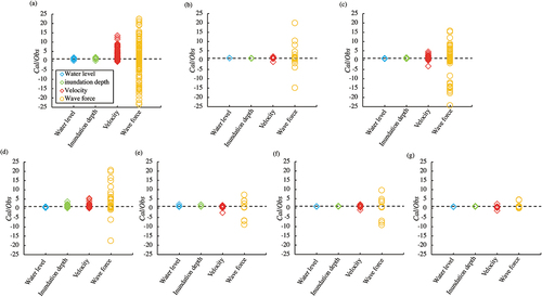
The authors first computed the ratio of calculated values to observed values for water levels, inundation depths, velocities, and wave forces. A Cal/Obs value closed to 1.0 indicates that the simulation results are in good agreement with the observation values. The Cal/Obs < 1.0 indicates that the simulation underestimates the observed values, and Cal/Obs > 1.0 indicates that the simulation overestimates the observed values. The values predicted by each model for tsunamis A and B are shown in Figures 11 and 12, respectively. In some cases, the values of Cal/Obs exceeded the ranges of the vertical axes of the diagrams especially for the 3D, 3D-NH, and 3D-H models, and could not be shown in the figure. In all methods, the Cal/Obs values for tsunami B were distributed far from 1.0 compared with that for tsunami A, indicating low prediction accuracy for tsunami B, where the tsunami was stronger and the dispersion effect was significant. For both tsunamis, the variability of Cal/Obs values was high in the nonhydrostatic incompressible fluid dynamics model (Figures 11 and 12) as this model had more cases than the other models (Table 2). The variabilities of the Cal/Obs values of the SPH were higher than those of the other models (Figures 11 and 12). Eight submitted results were calculated using the NSEW models (Table 4), while the Cal/Obs values of the NSWE models are not widely distributed in both tsunami A and B (Figures 11 and 12). The Cal/Obs values of the Boussinessq model also appeared not to be widely distributed (Figures 11 and 12); however, only one submission used this model (Table 2).

Figure 11. The ratio of calculated values and observed values (Cal/Obs) at all observation sites for tsunami A. The simulation results of (a) Nonhydrostatic incompressible fluid dynamics model, (b) Nonhydrostatic compressible fluid dynamics model, (c) Nonlinear shallow water equation model, (d) SPH, (e) Three-dimensional and non-hydrostatic model, (f) Three-dimensional and multilayer hydrostatic model, and (g) Nonlinear dispersive wave model are shown.

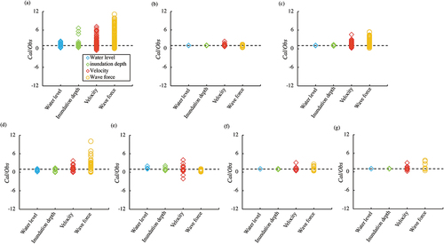
Figure 12. The ratio of calculated values and observed values (Cal/Obs) at all observation sites for tsunami B. The simulation results of (a) Nonhydrostatic incompressible fluid dynamics model, (b) Nonhydrostatic compressible fluid dynamics model, (c) Nonlinear shallow water equation model, (d) SPH, (e) Three-dimensional and non-hydrostatic model, (f) Three-dimensional and multilayer hydrostatic model, and (g) Nonlinear dispersive wave model are shown.

3.2. Detailed analysis of the submitted results

3.2.1. Results of Cal/Obs

The results of the detailed analysis of the Cal/Obs values of water level, inundation depth, velocity, and wave force versus distance from the shoreline are shown in Figures 13–16. To obtain the Cal/Obs of the wave force, the authors used the Cal/Obs values at P1-1 (0.5 m), P4-1 (1.25 m), P2-3 (2.0 m), P5-1 (2.4 m), and P3-1 (4.3 m), which were the frontal points against the tsunami propagation in the wave tank. The Cal/Obs at P4 and P5 were also provided to evaluate the reproducibility of tsunami wave forces acting on the sides and behind the structure (Figure 17). The wave pressure at P4 and P5 calculated using the Boussinesq model was not submitted; therefore, the Cal/Obs predicted by Boussinesq model is not shown in Figure 17. The authors also analyzed the Cal/Obs values of water level, inundation depth, velocity, and wave force versus grid cell size used in 3D and NSWE models (Figures 18 and 19). The authors excluded the Boussinesq model as only one case was submitted. The Cal/Obs values versus turbulence model used in 3D models are shown in Figures 20 and 21.

Figure 13. The ratio of calculated and observed water levels at −41.54 m (WG3), −30.0 m (WG4), −20.0 m (WG5), −10.0 m (WG6), −5.0 m (WG7), and 0.0 m (WG8) from the shoreline in the case of (a) tsunami A and (b) tsunami B.

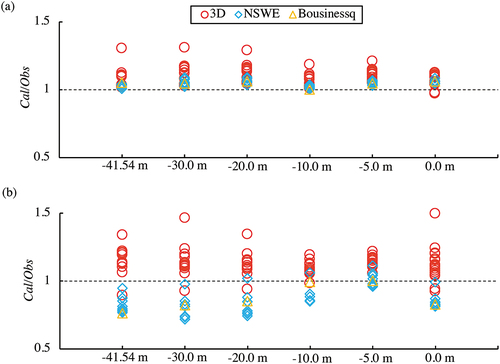
Figure 14. The ratio of calculated and observed inundation depths at 0.0 m, 0.4 m, 1.15 m, 1.90 m, 3.15 m, 4.15 m, and 4.75 m from the shoreline in the case of (a) tsunami A and y = 1.8 m, (b) tsunami A and y = 2.6 m, (c) tsunami B and y = 1.8 m, and (d) tsunami B and y = 2.6 m.

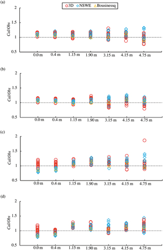
Figure 15. The ratio of calculated and observed velocities at 0.0 m, 0.4 m, 1.15 m, 1.90 m, 3.15 m, 4.15 m, and 4.75 m from the shoreline in the case of (a) tsunami A and y = 1.8 m, (b) tsunami A and y = 2.6 m, (c) tsunami B and y = 1.8 m, and (d) tsunami B and y = 2.6 m.

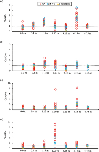
Figure 16. The ratio of calculated and observed wave forces at 0.5 m, 1.25 m, 2.0 m, 2.4 m, and 4.3 m from the shoreline in the case of (a) tsunami A and (b) tsunami B.

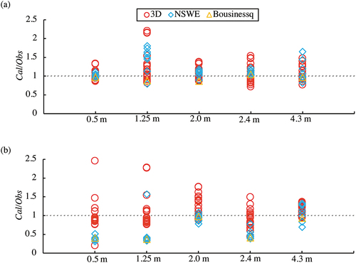
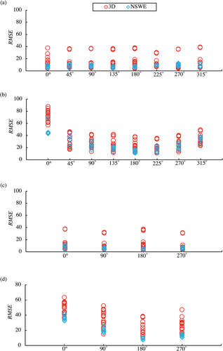
Figure 17. The ratio of calculated and observed wave forces at 0°, 45°, 90°, 135°, 180°, 225°, 270°, and 315° of P4 in the case of (a) tsunami A and (b) tsunami B. The ratio of calculated and observed wave forces at 0°, 90°, 180°, and 270° of P5 in the case of (c) tsunami A and (d) tsunami B are also shown.

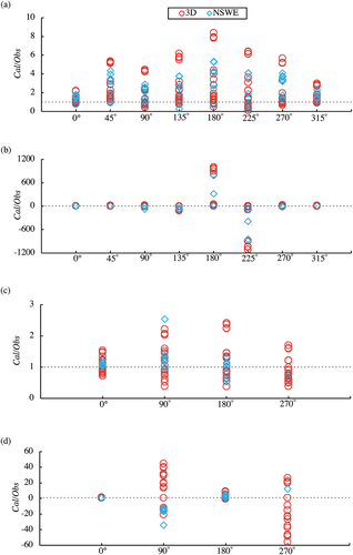
Figure 18. The ratio of calculated and observed values of (a) water levels, (b) inundation depths, (c) velocities, and (d) wave forces at all observation sites versus grid-cell size by 3D model and NSWE models in the case of tsunami A.

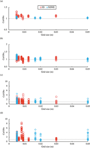
Figure 19. The ratio of calculated and observed values of (a) water levels, (b) inundation depths, (c) velocities, and (d) wave forces at all observation sites versus grid-cell size by 3D model and NSWE models in the case of tsunami B.

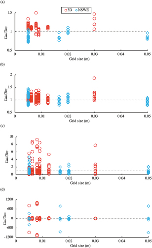
Figure 20. The ratio of calculated and observed values of (a) water levels, (b) inundation depths, (c) velocities, and (d) wave forces at all observation sites versus turbulence model used in the 3D model for Tsunami A. Models 1, 2, 3, 4, and 5 indicates without turbulence model (Laminar flow), dynamic k equation model in LES, Smagorinsky model in LES, standard k-εmodel in RANS, and stabilized k-ω in RANS, respectively.

Figure 21. The ratio of calculated and observed values of (a) water levels, (b) inundation depths, (c) velocities, and (d) wave forces at all observation sites versus turbulence model used in the 3D model for Tsunami B. Models 1, 2, 3, 4, and 5 indicates without turbulence model (Laminar flow), dynamic k equation model in LES, Smagorinsky model in LES, standard k-εmodel in RANS, and stabilized k-ω in RANS, respectively.

The Cal/Obs of water level (Figure 13) calculated for the 3D models were 0.97–1.31 and 0.89–1.50 for tsunamis A and B, respectively. The Cal/Obs for the NSWE model were 1.0–1.09 for tsunami A and 0.72–1.13 for tsunami B. The Cal/Obs for the Bousinessq model were 1.0–1.06 for tsunami A, and 0.72–1.11 for tsunami B (Figure 13). For tsunami A, where soliton fission was not generated, the water level could be simulated based on the hydrostatic assumption. Thus, the Cal/Obs calculated for the NSWE model was close to 1.0, compared with that for the 3D model. However, for tsunami B, the Cal/Obs of the NSWE model significantly decreased from 1.0 because the hydrostatic assumption cannot consider short-wave components such as soliton fissions.

The Cal/Obs calculated for the Boussinessq model for tsunami B was close to 1.0 compared to those for the NSWE model. The Cal/Obs for the Boussinessq model for tsunami B was lower than that for tsunami A. The decrease in Cal/Obs calculated for the 3D model for tsunami B was not significant compared to that for the NSWE and Boussinessq models. Thus, the prediction accuracy of the water level was not significantly decreased even if soliton fission was generated in the case of 3D model.

For tsunami A, the Cal/Obs values of simulated inundation depth at 0.0–1.90 m were close to 1.0 compared to those at 3.15–4.75 m (Figure 14). At 0.0–1.90 m, the flow stagnation was generated by blockage due to the buildings located behind 1.90 m. Thus, for tsunami A, the inundation depth at 0.0–1.90 m was uniform, approximately 0.15 m (Kihara et al. 2021). From 1.90 m toward inland, the inundation depth decreased, and the Cal/Obs was distributed in a wide range at 3.15–4.75 m where the inundation depth was less than 0.1 m (Kihara et al. 2021). For tsunami B, the inundation depth decreased from the shoreline toward inland, and the Cal/Obs were also distributed in wide range at 3.15–4.75 m in all models where the inundation depth was less than 0.1 m (Figures 14c and 14d). For tsunamis A and B, the reproducibility of the simulation models decreased as the inundation depth decreased.

In the case of velocity of tsunami A, the Cal/Obs values were widely distributed at 4.15 m of y = 1.8 m (Figure 15(a)). In the case tsunami B, the Cal/Obs were widely distributed at 1.90 m of y = 2.6 m (Figure 15d). At these sites, the tsunami velocities were significantly lower or higher compared to the other sites. For example, the velocity of tsunami A (y = 1.8 m) at 4.15 m was 0.213 m/s, while at 4.75 m, it was 1.02 m/s (Kihara et al. 2021).

The tsunami wave force has three phases (Arikawa et al. 2006; Nouri et al. 2010; Palermo et al. 2013; Kihara et al. 2015). In the first phase, an impulsive force is observed immediately after the bore impacts the structure. In the second phase (the transition or initial reflection phase), both hydrostatic and hydrodynamic forces contribute to the tsunami wave pressure. In the third phase (quasi-steady-state phase), the vertical distribution of the wave pressure appears to be hydrostatic. For tsunami A, the maximum wave force was observed in the third phase at all observation points (P1–P5). For tsunami B, the maximum wave force of the first or second phase was observed at P1-P5 (at 0–1.25 m) (Kihara et al. 2021). The 3D and NSWE models well reproduced the wave forces acting on P4 and P5 at 0° for both tsunamis with Cal/Obs close to 1.0 (Figure 17). However, the both models could not reproduce the wave forces on the rest of the points, P4 at 45–315° and P5 at 90–270°, with higher Cal/Obs. In the case of tsunami B, at places where a negative wave pressure was generated, the Cal/Obs values were negative.

Even if the grid-cell size was changed, a characteristic increase or decrease in the Cal/Obs was not observed in the both 3D and NSWE models (Figures 18 and 19). In LES, the Cal/Obs of wave force was close to 1.0 in the case of the dynamic k equation model compared to the Smagorinsky model for Tsunamis A and B (Figures 20 and 21). In RANS, the Cal/Obs of water level and wave force was close to 1.0 in the case of the k-ε model compared to the k-ω model for both Tsunamis (Figures 20 and 21).

3.2.2. The results of K and$\kappa$

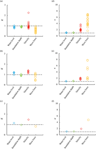
The K-$\kappa$ values of the 3D, NSWE, and Boussinesq models for tsunamis A and B are shown Figures 22 and 23, respectively. The K values were close to 1.0 for tsunami A compared with those for tsunami B. Further, the $\kappa$ values for tsunami B were higher compared to those for tsunami A, indicating high variabilities in the computational results of tsunami B.

Figure 22. The K values for (a) 3D model, (b) NSWE model, and (c) Boussinesq model at all observation sites for tsunami A. The κ values for (d) 3D model, (e) NSWE model, and (f) Boussinesq model at all observation sites for tsunami A are also shown.

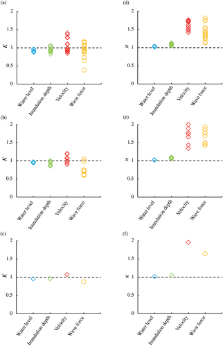
Figure 23. The K values for (a) 3D model, (b) NSWE model, and (c) Boussinesq model at all observation sites for tsunami B. The κ values for (d) 3D model, (e) NSWE model, and (f) Boussinesq model at all observation sites for tsunami B are also shown.

The authors calculated the $\kappa$ values of water level, inundation depths, velocity, and wave force from the shoreline toward downstream (Figures 24–27). The Boussinesq model was excluded as only one case was submitted. In all the cases, the $\kappa$ values for tsunami A were lower than those for tsunami B. For tsunami A, the $\kappa$ values of the water level in the NSEW models were lower than those in the 3D models at all observation points (Figure 24a). For tsunami B, the NSWE models had high $\kappa$ values of the 3D at four out of six points (Figure 24b), indicating that the NSWE model did not simulate tsunami B waveform properly. For both tsunamis, the $\kappa$ values of inundation depths were high at 3.15 m, 4.15 m, and 4.75 m, where the inundation depth was small (Figure 25). With regard to the velocities, the $\kappa$ values of NSWE models were low at 9 out of 14 points for tsunami A and at 13 out of 14 points for tsunami B (Figure 26). 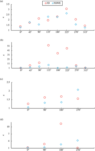Similarly, for tsunami wave forces, the $\kappa$ values of the NSWE models were low at 29 points among the 34 points for both tsunamis A and B (Figures 27 and 28). At most points of P4 and P5, the $\kappa$ values of the NSWE models were lower than those of the 3D models (Figure 28).

Figure 24. The κ values of water levels at −41.54 m (WG3), −30.0 m (WG4), −20.0 m (WG5), −10.0 m (WG6), −5.0 m (WG7), and 0.0 m (WG8) from the shoreline in the case of (a) tsunami A and (b) tsunami B.

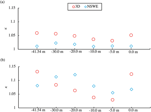
Figure 25. The κ values of inundation depths at 0.0 m, 0.4 m, 1.15 m, 1.90 m, 3.15 m, 4.15 m, and 4.75 m from the shoreline in the case of (a) tsunami A and y = 1.8 m, (b) tsunami A and y = 2.6 m, (c) tsunami B and y = 1.8 m, and (d) tsunami B and y = 2.6 m.

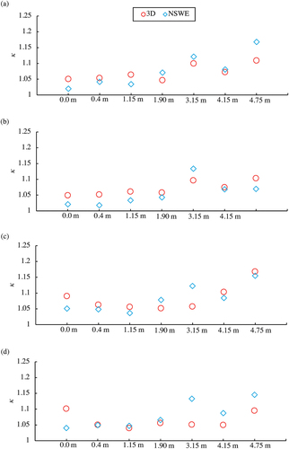
Figure 26. The κ values of velocities at 0.0 m, 0.4 m, 1.15 m, 1.90 m, 3.15 m, 4.15 m, and 4.75 m from the shoreline in the case of (a) tsunami A and y = 1.8 m, (b) tsunami A and y = 2.6 m, (c) tsunami B and y = 1.8 m, and (d) tsunami B and y = 2.6 m.

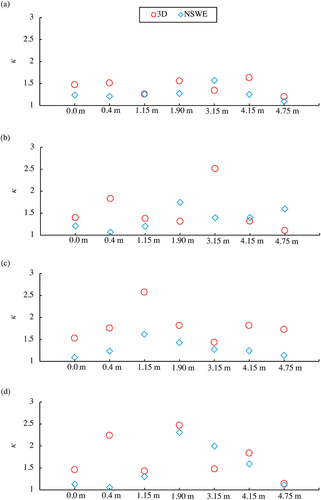
Figure 27. The κ values of wave forces at 0.5 m, 1.25 m, 2.0 m, 2.4 m, and 4.3 m from the shoreline in the case of (a) tsunami A and (b) tsunami B.

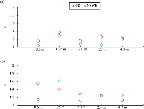
Figure 28. The κ values of wave forces at 0°, 45°, 90°, 135°, 180°, 225°, 270°, and 315° of P4 in the case of (a) tsunami A and (b) tsunami B. The ratio of calculated and observed wave forces at 0°, 90°, 180°, and 270° of P5 in the case of (c) tsunami A and (d) tsunami B are also shown.

Furthermore, the authors calculated the $\kappa$ values of water level, inundation depths, velocity, and wave forces versus grid-cell size (Figures 29 and 30) and turbulence model in 3D models (Figures 31 and 32). When coarse grid-cell sizes were used, the $\kappa$ values calculated for water levels and inundation depths in NSWE models were small for both Tsunamis (Figure 29), while the corresponding $\kappa$ values in 3D models were small for Tsunami A (Figure 30). In the case of velocity and wave force, a characteristic decrease or increase in $\kappa$ values was not found. In the case of dynamic k equation model, the $\kappa$ values for wave force were small compared to those in the Smagorinsky model in LES for Tsunamis A and B (Figures 31 and 32). The $\kappa$ values of wave force were small in the case of k-ε model compared to that of k-ω model in RANS for Tsunamis A and B (Figures 31 and 32). The $\kappa$ values of velocity in k-ω model were significantly high for Tsunami B because some calculated values were close to zero (Figure 20c).

Figure 29. The κ values of (a) water levels, (b) inundation depths, (c) velocities, and (d) wave forces at all observation sites versus grid-cell size by 3D and NSWE models in the case of tsunami A.

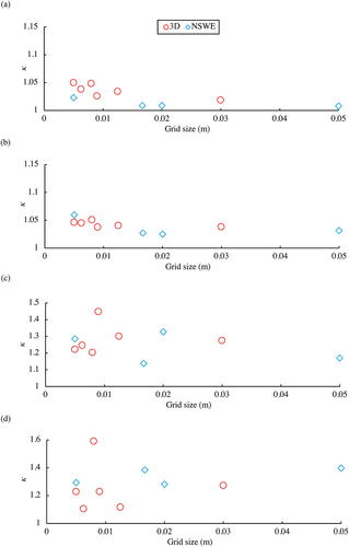
Figure 30. The κ values of (a) water levels, (b) inundation depths, (c) velocities, and (d) wave forces at all observation sites versus grid-cell size by 3D and NSWE models in the case of tsunami B.

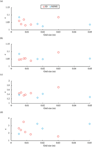
Figure 31. The κ values of (a) water levels, (b) inundation depths, (c) velocities, and (d) wave forces at all observation sites versus turbulence model used in the 3D model for Tsunami A. Models 1, 2, 3, 4, and 5 indicates without turbulence model (Laminar flow), dynamic k equation model in LES, Smagorinsky model in LES, standard k-εmodel in RANS, and stabilized k-ω in RANS, respectively.

Figure 32. The κ values of (a) water levels, (b) inundation depths, (c) velocities, and (d) wave forces at all observation sites versus turbulence model used in the 3D model for Tsunami B. Models 1, 2, 3, 4, and 5 indicates without turbulence model (Laminar flow), dynamic k equation model in LES, Smagorinsky model in LES, standard k-εmodel in RANS, and stabilized k-ω in RANS, respectively.

3.2.3. The results of RMSE

To evaluate the reproducibility of the calculated waveform, the authors computed the RMSE values of water level, inundation depths, velocity, and wave force from the shoreline toward the inland obtained from the 3D, NSWE, and Boussinesq models for tsunamis A and B (Figures 33–36). The RMSE values at P4 and P5 were also calculated (Figure 37). The RMSE values for tsunami B were higher compared to those for tsunami A at most points (Figures 33–36). Some RMSE values of the 3D models were significantly higher because of the inconsistencies in the predicted results (Figures 33–36). The RMSE values of inundation depth calculated for all models decreased inland for both tsunamis (Figure 34), indicating good agreement between calculated waveforms and the observed ones when the inundation depth was low. The RMSE values of velocities increased inland for both tsunamis (Figure 35), indicating high prediction accuracy when the inundation depth was high. The RMSE values predicted for the NSWE for wave force were much lower than those predicted for the 3D model (Figures 36 and 37). For tsunami B, at 0° of P4 and P5, where the wave force was high, the RMSE values also increased compared with other points (Figures 37(b, d)).

Figure 33. The RMSE values of water levels at −41.54 m (WG3), −30.0 m (WG4), −20.0 m (WG5), −10.0 m (WG6), −5.0 m (WG7), and 0.0 m (WG8) from the shoreline in the case of (a) tsunami A and (b) tsunami B.

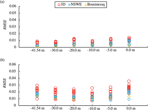
Figure 34. The RMSE values of inundation depths at 0.0 m, 0.4 m, 1.15 m, 1.90 m, 3.15 m, 4.15 m, and 4.75 m from the shoreline in the case of (a) tsunami A and y = 1.8 m, (b) tsunami A and y = 2.6 m, (c) tsunami B and y = 1.8 m, and (d) tsunami B and y = 2.6 m.

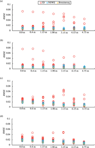
Figure 35. The RMSE values of velocities at 0.0 m, 0.4 m, 1.15 m, 1.90 m, 3.15 m, 4.15 m, and 4.75 m from the shoreline in the case of (a) tsunami A and y = 1.8 m, (b) tsunami A and y = 2.6 m, (c) tsunami B and y = 1.8 m, and (d) tsunami B and y = 2.6 m.

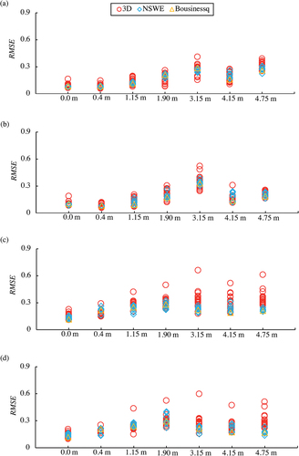
Figure 36. The RMSE values of wave forces at 0.5 m, 1.25 m, 2.0 m, 2.4 m, and 4.3 m from the shoreline in the case of (a) tsunami A and (b) tsunami B.

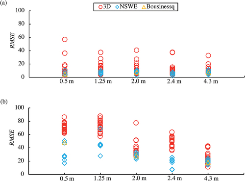
Figure 37. The RMSE values of wave forces at 0°, 45°, 90°, 135°, 180°, 225°, 270°, and 315° of P4 in the case of (a) tsunami A and (b) tsunami B. The ratio of calculated and observed wave forces at 0°, 90°, 180°, and 270° of P5 in the case of (c) tsunami A and (d) tsunami B are also shown.

The RMSE values versus grid-cell sizes and turbulence models used in 3D models are shown in Figures 38–41. The Boussinesq model was excluded as only one case was submitted. A characteristic increase or decrease in RMSE values was not observed with varying grid-cell sizes (Figure 39).

Figure 38. The RMSE values of (a) water levels, (b) inundation depths, (c) velocities, and (d) wave forces at all observation sites versus grid-cell size by 3D and NSWE models in case of tsunami A.

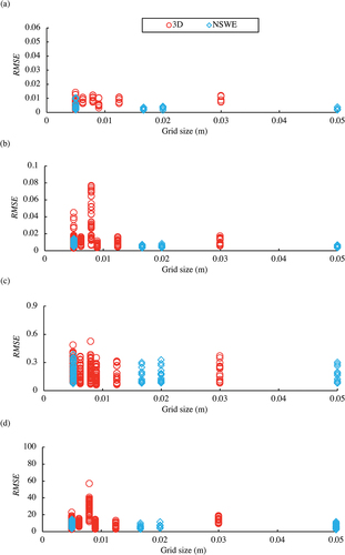
Figure 39. The RMSE values of (a) water levels, (b) inundation depths, (c) velocities, and (d) wave forces at all observation sites versus grid-cell size by 3D and NSWE models in case of tsunami B.

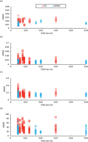
Figure 40. The RMSE values of (a) water levels, (b) inundation depths, (c) velocities, and (d) wave forces at all observation sites versus turbulence model used in the 3D model for Tsunami A. Models 1, 2, 3, 4, and 5 indicates without turbulence model (Laminar flow), dynamic k equation model in LES, Smagorinsky model in LES, standard k-εmodel in RANS, and stabilized k-ω in RANS, respectively.

Figure 41. The RMSE values of (a) water levels, (b) inundation depths, (c) velocities, and (d) wave forces at all observation sites versus turbulence model used in the 3D model for Tsunami B. Models 1, 2, 3, 4, and 5 indicates without turbulence model (Laminar flow), dynamic k equation model in LES, Smagorinsky model in LES, standard k-εmodel in RANS, and stabilized k-ω in RANS, respectively.

The RMSE values of inundation depth, velocity, and wave forces were close to zero in dynamic k equation model compared to those in Smagorinsky model in LES for both Tsunamis (Figure 40). In RANS, the RMSE values of water level, inundation depth, and velocity were close to zero in k-ε model compared to k-ω model (Figure 41).

4. Discussion

4.1. The reproductivity of maximum values

In the SPH methods, the Cal/Obs values of the four outputs (water level, inundation depth, wave pressure, and wave velocity) were widely distributed for both tsunami A and B (Figures 11 and 12). In the case of the SPH method, determining the free water surface is challenging. Therefore, the calculated time series of outputs oscillated and the Cal/Obs of these simulation results were quite far from 1.0. Only one case of prediction was submitted for both 3D-NH and 3D-H models. More cases must be analyzed to reveal the reproducibility of the tsunami simulation from both models. The submitted NSWE models were second-highest in number among the seven models (Table 2). However, the calculated Cal/Obs values for the NSWE models were not widely distributed for both tsunamis compared to that for the 3D models (Figures 11 and 12). This result can be attributed to the fact that in the case of NSWE model, the stability of the difference scheme has been theoretically investigated and numerical errors and their causes in the model are also clear (Shigihara and Fujima 2007). The Cal/Obs values for the Bousinessq models were also close to 1.0, as only one case of prediction results was used for calculations (Figures 11 and 12); more prediction cases are required to assess the accuracy of the model.

4.2. Reproducibility of NSWE and 3D models

The Cal/Obs values of water level calculated by the NSWE model are significantly smaller in Tsunami B as compared to Tsunami A. Meanwhile, the Cal/Obs values of 3D models in Tsunami B are not as small as those produced by the NSWE models (Figure 13). For Tsunami B, the $\kappa$ values of water levels were smaller in 3D models than those in NSWE models in most cases (Figure 24). Therefore, in the computation of tsunami propagation where short waves are present, 3D models are valid. To study the tsunami inundation over urban areas, where the local water level change is significant, it is important to consider the non-hydrostatic behavior (Watanabe et al. 2016). The $\kappa$ values of inundation depth calculated for the 3D models were close to 1.0 as compared to those for the NSWE models for both tsunamis at 1.15 − 4.75 m where the observation points were surrounded by structures (Figure 25). The velocity and wave force variabilities calculated for the 3D models were higher than those for the NSWE models (Figures 26–28). The NSWE models cannot directly calculate wave pressures, hence some empirical models (e.g. Arimitsu, Ooe, and Kawasaki 2012) were used to derive wave pressure or wave force. 3D models can consider these effects. For tsunami A, maximum wave force was observed in the third phase at all observation points (Kihara et al. 2021), which implies that maximum wave force can be calculated, based on the hydrostatic assumption, using the NSWE model and reproduced with reasonable accuracy.

For tsunami B, the maximum wave force of the first or second phase, because of impulsive pressure or hydrodynamic pressure, was observed at all observation points (Kihara et al. 2021). However, the $\kappa$ values for the 3D models were higher than those for the NSWE model at most points (Figures 27 and 28). The variabilities of the calculated wave force behind P4 and P5 were also significantly higher in the 3D models than in the NSWE models (Figure 28). Thus, the simulation results calculated by the NSWE models were more accurate compared to the 3D models.

The RMSE values of water level, inundation depth, velocity, and wave force were mostly low in the NSWE model for tsunami A(Figures 33–37). Similarly, for tsunami B, most RMSE values were low in the NSWE model compared to the 3D model. Thus, the reproducibility of the time series of the tsunami water level, inundation depth, velocity, and wave force calculated by the NSWE models were higher than those by the 3D models. The NSWE models can stably conduct the calculation compared to 3D models. In the case of the 3D model, some results had outliers. The RMSE values were calculated from the squared values of the difference between the calculated value and the measured values (Equation 4(4) $RMSE=\sqrt{\frac{1}{n}\sum _{i=1}^n{\left(Obs-Cal\right)}^2}$(4) ), making the RMSE values sensitive toward outliers.

Meanwhile, the simulation of flows on underwater vehicle appendages using dynamic k-equation models of LES has produced better results compared to the Smagorinsky models because the size and position of the separation bubble were reproduced better in the former than in the latter model (Lidtke, Turnock, and Downes 2017). The dynamic k equation model is more advanced than the Smagorinsky model and is necessary to solve the transport equation for the subgrid turbulent kinetic energy (Kim and Menon 1995). In the present study, the RMSE values of the inundation depths, velocities, and wave forces calculated using dynamic k equation model were close to zero compared to the Smagorinsky model for both Tsunamis (Figures 40 and 41). Furthermore, the $\kappa$ values of wave forces were lower in the dynamic k equation model than those in the Smagorinsky model in LES for both Tsunamis (Figures 31 and 32).

Moreover, the tsunami wave force acting on bridges and time series of wave levels were reproduced well when the k-ω model was adopted compared to the k-ε model because the former is more suitable for the calculation of separated flows than the latter (Kawasaki, Nakao, and Izuno 2015). However, in this study, the $\kappa$ values of wave force were small in the k-ε model than those in the k-ω model (Figures 31 and 32). The RMSE values of water levels, inundation depths, and velocities calculated for the k-ε model were also close to zero compared to those for the k-ω model for both tsunamis (Figures 40 and 41). This is because the stability of the k-ε model is higher than that of the k-ω model (Kawasaki, Nakao, and Izuno 2015).

4.3. Future improvements in the tsunami simulation model

The SPH method uses a meshless approach to simulate the inundation of wave breaking and other flows (Rogers and Dalrymple 2008). However, it requires more computation time than the mesh approach (e.g. Genda et al., 2015). Moreover, its computation accuracy become low at the area with few particles such as the location where water depth become small. Thus, further development of the SPH method is necessary. The NSWE models cannot simulate three-dimensional flows; therefore, the tsunami inundation among the structures and wave forces acting on the sides or backside of the structures cannot be reproduced. However, the accuracy of the NSWE models was higher than that of the 3D models. The NSWE models are commonly used for tsunami simulations, and the parameters setting that can reproduce tsunami inundation and propagation has been empirically recognized. The 3D models are not commonly used; therefore, the parameter setting and selection of turbulence models are varied with each user. However, the NSWE model cannot handle some phenomena, such as soliton fission and vertical flows in front of the structures. Therefore, the further development and use of 3D models are necessary.

The accuracy of simulation results did not increase even when the grid cell-size was small in the both NSWE model and 3D models (Figures 18–19), (Figures 29–30), (Figures 38–39). Especially, in case of the NSWE model, the κ values of water level and inundation depths increased at small grid-cell sizes for Tsunamis A and B (Figures 29–30). Thus, not only the grid-cell size but also other parameters contribute to the reproducibility of the tsunami simulation results. Thus, it is necessary to assess the input parameters to accurately perform tsunami inundation modeling are necessary to be revealed in the future.

Among the 24 submitted results of the 3D models, 23 were incompressible models and one was a compressible model (Table 2), implying that the compressible model was not widespread. However, the tsunami propagation speed is also affected by compressible seawater (Tsai et al. 2013; Watada et al. 2013). The tsunami propagation speed was reduced by 0.44% when seawater compressibility was not included (Watada 2013). Therefore, to increase the reproducibility of tsunami propagation, further development of a compressible 3D model is required.

5. Conclusion

To date, several tsunami simulation methods have been developed. To confirm the accuracy of the proposed numerical models, the authors held a tsunami blind contest, which was part of the 17WCEE. In this study, the authors compared the accuracies of the simulation results submitted by the participants. The main outcomes as follows:

• Reproducibility of water level, inundation depth, and velocity

The reproducibility of water level value was higher in the 3D model than in the NSWE models when soliton fission was generated. In the case of inundation depth, the prediction accuracy of the 3D model was higher than that of the NSWE models as the tsunami inundation among structures is a three-dimensional problem. The reproducibility of velocity were lower in the 3D models than in the NSWE models.

• Reproducibility of pressure/forces

In this study, NSWE models were much better able to reproduce wave force over land as compared to 3D models. For both Tsunami A and B, wave forces in all phases of the tsunami, including significant impulsive pressure and hydrodynamic pressure, were more accurately predicted by the NSWE models. The variability of the calculated wave force of the behind structures in 3D models was also significantly higher than that in the NSWE models. Although the 3D models can directly solve these wave forces, but the simulation results calculated by the NSWE models were more accurate than those with the 3D models.

• Effects of grid-cell size and turbulence model in tsunami modeling

The reproducibility of 3D models and NSWE models did not improve at small grid-cell sizes. Thus, the grid-cell size was not the factor to determine the simulation accuracy. For 3D models in RANS, simulation accuracy increased in cases where k-ε model was adopted compared to the cases where k-ω model was used. For 3D models in LES, reproducibility of wave force was higher in the dynamic k equation model than that in the Smagorinsky model.

• Limitations and improvements of current numerical simulation models

To improve the accuracy of numerical models that can directly solve wave pressure, such as 3D model and the SPH models, further developments are needed. The appropriate parameter setting for tsunami inundation modeling is still unknown and should be investigated in the future.

The presented information will contribute to the development of numerical simulation tools that can accurately predict tsunami inundation and its hydraulic force.

Acknowledgments

The authors acknowledge the 14 participants for performing simulations and analyses, and discussing their results, and summarizing their technical reports.

Disclosure statement

No potential conflict of interest was reported by the author(s).

Supplementary material

Supplemental data for this article can be accessed online at https://doi.org/10.1080/21664250.2022.2072611

References

- Abualtayef, M, M Kuroiwa, K Tanaka, Y Matsubara, and J. Nakahira. 2008. “Three-dimensional Hydrostatic Modeling of a Bay Coastal Area.” Journal of Marine Science and Technology 13 (1): 40–49. doi:https://doi.org/10.1007/s00773-007-0257-6.
- AdvanceSoft. “Fluid Analysis Software Advance/FrontFlow/red. Undated. Available At.” Japanese, Accessed 26 January 2022. https://www.advancesoft.jp/product/advance_frontflow_red/
- Aida, I. 1978. “Reliability of Tsunami Source Model Derived from Fault Parameters.” Journal of Physics of the Earth 26 (1): 57–73. doi:https://doi.org/10.4294/jpe1952.26.57.
- Arikawa, T, D Ohtubo, F Nakano, K Shimosako, S Takahashi, F Imamura, and H. Matsutomi. 2006. “Large Model Test on Surge Front Tsunami Force”. Coastal Engineering, Japan Society of Civil Engineers 53 796–800. in Japanese
- Arikawa, T, T Yamano, and M. Akiyama. 2007. “Advanced Deformation Method for Breaking Wave by Using CADMAS-SURF/3D.” Coastal Engineering, Japan Society of Civil Engineers 54: 71–75. Japanese.
- Arikawa, T, N Ishikawa, M Beppu, and H. Tatesawa. 2012. “Collapse Mechanisms of Seawall Due to the March 2011 Japan Tsunami Using the MPS Method.” International Journal of Structure 3 (4): 457–476. doi:https://doi.org/10.1260/2041-4196.3.4.457.
- Arikawa, T, N Kihara, M Watanabe, C Tsurudome, M Hasebe, Y Shigihara, T Asai, et al. 2021. “Blind Prediction Contest for Tsunami Inundation and Impact.” Proceeding of 17th World Conference on Earthquake Engineering, Sendai, September.
- Arimitsu, T, K Ooe, and K. Kawasaki. 2012. “Proposal of Evaluation Method of Tsunami Wave Pressure Using 2D Depth-Integrated Flow Simulation.”Coastal Engineering, Japan Society of Civil Engineers 68 (2) I_781–I_785 in Japanese
- Choi, BH, E Pelinovsky, DC Kim, KO Kim, and KH. Kim. 2008. “Three-dimensional Simulation of the 1983 Central East (Japan) Sea Earthquake Tsunami at the Imwon Port (Korea).” Ocean English 35 (14–15): 1545–1559. doi:https://doi.org/10.1016/j.oceaneng.2008.06.002.
- Christophe, L, O Scotti, and M. Ioualalen. 2012. “Reappraisal of the 1887 Ligurian Earthquake (Western Mediterranean) from Macroseismicity, Active Tectonics and Tsunami Modelling.” Geophysical Journal International 190 (1): 87–104. doi:https://doi.org/10.1111/j.1365-246X.2012.05498.x.
- Flow Science. “FLOW3D-Hydro Version 12.0 User’s Manual Computer Software.” Undated. Accessed date26 January 2022. Available at. https://www.flow3d.com/
- Gica, E, VV Titov, C Moore, and Y Wei. 2015. “Tsunami Simulation Using Sources Inferred from Various Measurement Data: Implications for the Model Forecast.” Pure and Applied Geophysics 172 (3–4): 773–789. doi:https://doi.org/10.1007/s00024-014-0979-4.
- Gusman, AR, Y Tanioka, BT MacInnes, and H. Tsushima. 2014. “A Methodology for Near-field Tsunami Inundation Forecasting: Application to the 2011 Tohoku Tsunami.” Journal of Geophysics Res. Solid Earth 119 (11): 8186–8206. doi:https://doi.org/10.1002/2014JB010958.
- Higuera, P, JL Lara, and IJ. Losada. 2013. “Realistic Wave Generation and Active Wave Absorption for Navier-Stokes Models: Application to OpenFOAM®.” Coastal Engineering 71: 102–118. doi:https://doi.org/10.1016/j.coastaleng.2012.07.002.
- Hirt, CW, and BD. Nichols. 1981. “Volume of Fluid (VOF) Method for the Dynamics of Free Boundaries.” Journal of Computational Physics 39 (1): 201–225. doi:https://doi.org/10.1016/0021-9991(81)90145-5.
- Huang, Y, and C. Zhu. 2015. “Numerical Analysis of Tsunami–structure Interaction Using a Modified MPS Method.” National Hazards 75 (3): 2847–2862. doi:https://doi.org/10.1007/s11069-014-1464-1.
- International Association for Earthquake Engineering. “17th World Conference on Earthquake Engineering.” undated, 26 January 2022. https://www.17wcee.jp/
- Joshi, A, S Arora, and K. Kamal. 2014. “Modeling of Strong Motion Generation Areas of the 2011 Tohoku, Japan Earthquake Using Modified Semi-empirical Technique.” National Hazards 71 (1): 587–609. doi:https://doi.org/10.1007/s11069-013-0922-5.
- Kawasaki, Y, H Nakao, and K. Izuno. 2015. “Multi-phase Flow Analysis of Tsunami Forces and Associated Pressures on a Rectangular-section Bridge Girder.” Journal of Japan Society of Civil Engineers 71 (2): 199–207. Japanese.
- Kihara, N, Y Niida, D Takabatake, H Kaida, A Shibayama, and Y. Miyagawa. 2015. “Large-scale Experiments on Tsunami-induced Pressure on a Vertical Tide Wall.” Coast Engeenering 99: 46–63. doi:https://doi.org/10.1016/j.coastaleng.2015.02.009.
- Kihara, N, T Arikawa, T Asai, M Hasebe, T Ikeya, S Inoue, H Kaida, et al. 2021. “A Physical Model of Tsunami Inundation and Wave Pressures for an Idealized Coastal Industrial Site.” Coast Engneering 169: 103970. doi:https://doi.org/10.1016/j.coastaleng.2021.103970.
- Kim, WW, and S. Menon. 1995. “A New Dynamic One-equation Subgrid-scale Model for Large Eddy Simulations.” 33rd Aerospace Sciences Meeting and Exhibit, Reno, NV, USA.
- Koçyigit, MB, AR Falconer, and B. Lin. 2002. “Three-dimensional Numerical Modelling of Free Surface Flows with Non-hydrostatic Pressure.” International Journal for Numerical Methods in Fluids 40 (9): 1145–1162. doi:https://doi.org/10.1002/fld.376.
- Koshimura, S, T Oie, H Yanagisawa, and F. Imamura. 2002. “Developing Fragility Functions for Tsunami Damage Estimation Using Numerical Model and Post-Tsunami Data from Banda Aceh, Indonesia.” Coastal Engineering Journal 51 (3): 243–273. doi:https://doi.org/10.1142/S0578563409002004.
- Koshizuka, S, and Y. Oka. 1996. “Moving-particle Semi-implicit Method for Fragmentation of Incompressible Fluid.” Nuclear Science and Engineering: The Journal of the American Nuclear Society 123 (3): 421–434. doi:https://doi.org/10.13182/NSE96-A24205.
- Launder, BE, and DB. Spalding. 1974. “The Numerical Computation of Turbulent Flows.” Computer Methods in Applied Mechanics and Engineering 3 (2): 269–289. doi:https://doi.org/10.1016/0045-7825(74)90029-2.
- Lidtke, AK, SR Turnock, and J. Downes. 2017. “Simulating Turbulent Transition Using Large Eddy Simulation with Application to Underwater Vehicle Hydrodynamic Modelling.” 20th Numerical Towing Tank Symposium, Wageningen, October.
- Lynett, P, PLF Liu, KI Sitanggang, and DH. Kim. 2002. “Modeling Wave Generation, Evolution, and Interaction with Depth Integrated Dispersive Wave Equations COULWAVE Code Manual.” Cornell University Long and Intermediate Wave Modeling Package.
- Macías, J, MJ Castro, and CE. Sánchez. 2020. “Performance Assessment of the Tsunami-HySEA Model for NTHMP Tsunami Currents Benchmarking. Laboratory Data.” Coastal Engineering 158: 103667. doi:https://doi.org/10.1016/j.coastaleng.2020.103667.
- MacInnes, BT, AR Gusman, RJ LeVeque, and Y. Tanioka. 2013. “Comparison of Earthquake Source Models for the 2011 Tohoku Event Using Tsunami Simulations and Near-field Observations.” Coastal Engineering 103 (2B): 1256–1274. doi:https://doi.org/10.1785/0120120121.
- Marras, S, and KT. Mandli. 2021. “Modeling and Simulation of Tsunami Impact: A Short Review of Recent Advances and Future Challenges.” Geosciences 11 (1): 5. doi:https://doi.org/10.3390/geosciences11010005.
- Mas, E, S Koshimura, A Suppasri, M Matsuoka, T Yoshii, C Jimenez, F Yamazaki, and F. Imamura. 2012. “Developing Tsunami Fragility Curves Using Remote Sensing and Survey Data of the 2010 Chilean Tsunami in Dichato.” Natural Hazards and Earth System Sciences 12 (8): 2709–2718.
- Mulia, IE, T Ishibe, K Satake, AR Gusman, and S. Murotani. 2020. “Regional Probabilistic Tsunami Hazard Assessment Associated with Active Faults along the Eastern Margin of the Sea of Japan.” Earth Planets Space 72 (1): 123. doi:https://doi.org/10.1186/s40623-020-01256-5.
- Nouri, Y, I Nistor, D Palermo, and A. Cornett. 2010. “Experimental Investigation of Tsunami Impact on Free Standing Structures.” Coastal Engineering Journal 52 (1): 43–70. doi:https://doi.org/10.1142/S0578563410002117.
- Palermo, D, I Nistor, T Al-Faesly, and A. Cornett. 2013. “Impact of Tsunami Forces on Structures.” Journal of Tsunami 32 (2): 58–76.
- Pietrzak, J, JB Jakobson, H Burchard, HJ Vested, and O. Petersen. 2002. “A Three-dimensional Hydrostatic Model for Coastal and Ocean Modelling Using A Generalised Topography following Co-ordinate System.” Ocean Modelling 4 (2): 173–205. doi:https://doi.org/10.1016/S1463-5003(01)00016-6.
- Rogers, BD, and RA. Dalrymple. 2008. “SPH Modeling of Tsunami Waves.” In Advanced Numerical Models for Simulating Tsunami Waves and Runup, edited by P. L.-F. Liu, H. Yeh, and C. Synolakis, 75–100 . Vol. 10. doi:https://doi.org/10.1142/9789812790910_0003.
- Sarfaraz, M, and A. Pak. 2017. “SPH Numerical Simulation of Tsunami Wave Forces Impinged on Bridge Superstructures.” Coast Engeenering 121: 145–157. doi:https://doi.org/10.1016/j.coastaleng.2016.12.005.
- Satake, K, and Y. Tanioka. 2003. “The July 1998 Papua New Guinea Earthquake: Mechanismand Quantification of Unusual Tsunami Generation.” Pure Appliacation of Geophyics 160 (10–11): 2087–2118. doi:https://doi.org/10.1007/s00024-003-2421-1.
- Shi, F, JT Kirby, JC Harris, JD Geiman, and ST. Grilli. 2012. “A High-order Adaptive Time-stepping TVD Solver for Boussinesq Modeling of Breaking Waves and Coastal Inundation.” Ocean Modelling 43: 36–51. doi:https://doi.org/10.1016/j.ocemod.2011.12.004.
- Shigihara, Y, and K. Fujima. 2007. “Adequate Numerical Scheme for Dispersive Wave Theory for Tsunami Simulation and Development of New Numerical Algorithm.” Doboku Gakkai Ronbunshu 63 (1): 51–66. doi:https://doi.org/10.2208/jscejb.63.51.
- Smagorinsky, J. 1963. “General Circulation Experiments with the Primitive Equations.” Weather Reverse 91 (3): 99–164. doi:https://doi.org/10.1175/1520-0493(1963)091<0099:GCEWTP>2.3.CO;2.
- Sugawara, D. 2020. “Trigger Mechanisms and Hydrodynamics of Tsunamis.” In Geological Records of Tsunamis and Other Extreme Waves, edited by M Engel, J Pilarczyk, M.S May, D Brill, and E Garrett, 143–168.
- Suppasri, A, S Koshimura, and F. Imamura. 2011. “Developing Tsunami Fragility Curves Based on the Satellite Remote Sensing and the Numerical Modeling of the 2004 Indian Ocean Tsunami in Thailand.” Natural Hazards and Earth System Sciences 11 (1): 173–189. doi:https://doi.org/10.5194/nhess-11-173-2011.
- Suppasri, A, E Mas, S Koshimura, K Imai, K Harada, and F. Imamura. 2012. “Developing Tsunami Fragility Curves from the Surveyed Data of the 2011 Great East Japan Tsunami in Sendai and Ishinomaki Plains.” Coastal Engineering Journal 54 (1): 1250008. doi:https://doi.org/10.1142/S0578563412500088.
- Synolakis, C.E, E.N Bernard, V.V Titov, U Kanoglu, and F.I. Gonzalez. OAR PMEL-135 Standards, Criteria, and Procedures for NOAA Evaluation of Tsunami Numerical Models, NOAA/Pacific Marine Environmental Laboratory, Seattle, WA.
- Tomita, T, and T. Kakinuma. 2005. “Development of Storm Surge/tsunami Numerical Simulator STOC considering Three-dimensionality of Ocean Water Flow and Its Application to Tsunami Analysis.” Report of the Port and Airport Research Institute 44 (2–5): 83–98.
- Tsai, VC, JP Ampuero, H Kanamori, and DJ. Stevenson. 2013. “Estimating the Effect of Earth Elasticity and Variable Water Density on Tsunami Speeds.” Geophysics 40 (3): 492–496. doi:https://doi.org/10.1002/grl.50147.
- Watada, S. 2013. “Tsunami Speed Variations in Density-stratified Compressible Global Oceans.” Geophysics 40 (15): 4001–4006. doi:https://doi.org/10.1002/grl.50785.
- Watanabe, Y, R Sakai, H Oyaizu, T Makita, K Morioka, and A. Saruwatari. 2016. “Application of a Moving Contact Model for Run-up Waves to Urban Flooding Process”. Coastal Engineering, Japan Society of Civil Engineers. in Japanese 72 2: I_67–I_72. https://doi.org/10.2208/kaigan.72.I_67.
- Watanabe, M, K Goto, JD Bricker, and F. Imamura. 2018. “Are Inundation Limit and Maximum Extent of Sand Useful for Differentiating Tsunamis and Storms? An Example from Sediment Transport Simulations on the Sendai Plain, Japan.” Sedimentary Geology 364: 204–216. doi:https://doi.org/10.1016/j.sedgeo.2017.12.026.
- Watts, P, F Imamura, and S. Grilli. 2011. “Comparing Model Simulations of Three Benchmark Tsunami Generation Cases.” Science of Tsunami Hazards 18: 2.
- Weller, HG, G Tabor, H Jasak, and C. Fureby. 1998. “A Tensorial Approach to Computational Continuum Mechanics Using Object-oriented Techniques.” Computers in Physics 12 (6): 620–631. doi:https://doi.org/10.1063/1.168744.
- Wijatmiko, I, and K. Murakami. 2010. “Three Dimensional Numerical Simulation of Bore Type Tsunami Propagation and Run up on to a Dike.” Journal of Hydrodynamics 22 (5): 259–264. doi:https://doi.org/10.1016/S1001-6058(09)60204-3.
- Wilco, DC. 2006. Turbulence Modeling for CFD. 3rd Edition ed. La Canada California: DCW Industries.
- Xie, J, I Nistor, and T. Murty. 2012. “A Corrected 3-D SPH Method for Breaking Tsunami Wave Modelling.” Nationa Hazards 60 (1): 81–100. doi:https://doi.org/10.1007/s11069-011-9954-x.