Performance of ERA5 wind speed and significant wave height within Extratropical cyclones using collocated satellite radar altimeter measurements

ABSTRACT

Similar in strength to hurricanes, Extratropical Cyclones (ECs) are responsible for innavigable sea states, coastal inundation and erosion, and subsequent destruction to coastal infrastructure. Across modern operational wave models, there exists a known systematic underestimation of wave heights during these extreme events. Using a global database of EC storm tracks and 36 years of satellite altimeter data, we examine EC structure and assess model performance through storm centered composite analyses of significant wave height ($H_s$) and U10 wind speed ($|\mathit{U}10|$). Through the collocation of satellite altimeter observations with a state-of-the-art reanalysis product (ERA5), we investigate model performance with respect to $|\mathit{U}10|$ and $H_s$ within ECs of varying intensities. By rotating our data reference frames, we align all storm directions to account for asymmetry in EC wind fields and subsequent increased wave growth This rotation results in the organization of the strongest wind speed and $H_s$, as well as trends in the ERA5 performance. A characteristic EC radii is calculated and used to normalize data coordinates in the storm centered reference frame, which highlights the organization of EC structures. Performance metrics are then compared within different EC quadrants to explore the relationship between wind forcing accuracy and underestimation of $H_s$.

KEYWORDS:

• Extratropical cyclones
• ERA5 reanalysis
• satellite radar altimeter
• wind speed
• significant wave height
• performance statistics

1. Introduction

Extratropical Cyclones (ECs) form along atmospheric fronts between cold and warm air masses in the mid to high latitudes, acting to mix polar air to the north with subtropical air to the south (vise-versa in the Southern Hemisphere). The structure of ECs includes a warm front at the leading edge of the warm, moist air mass traveling poleward as it is advected around the storm, and a cold front marking the edge of the cold air mass being advected equatorward. Strong low-level winds, referred to as cold and warm jets, are often associated with the rapid movement of the cold and warm air masses around these storms. Although very rare, a shorter-lived, narrow region of extreme surface winds, called a sting jet, can also appear positioned in the back half of the storm, directly behind the bend in the advancing cold front (Browning 2004). The organization of these structures are known to vary substantially in intensity and orientation not only from storm to storm but also within a single EC lifetime as each storm develops, reaches its maximum intensity, and finally weakens (Hewson and Neu 2015; Ponce de León and Bettencourt 2021). Different cyclone regions, most notably those associated with the warm jet and cold jet, have been shown to uniquely influence momentum input into the upper ocean and are capable of producing hazardous conditions for coastal infrastructure and maritime travel (Bell, Gray, and Jones 2017; Hewson and Neu 2015; Kita, Waseda, and Webb 2018).

Asymmetry of cyclone wind fields, caused by the alignment of winds and storm translational velocity in the cyclone region to the right (left in the Southern Hemisphere) of the storm’s forward movement, often generates the largest waves. This is due to extreme winds and a phenomena known as dynamic, or extended fetch, which describes the resonant effects that occur when cyclone velocity is similar to the group velocity of the generated surface gravity waves. This prolonged exposure enhances the momentum input from wind to waves over a larger effective fetch both spatially and temporally (Hell, Ayet, and Chapron 2021; Kita, Waseda, and Webb 2018; Young and Vinoth 2013). With the large abundance of these storms that occur on a yearly basis and their capacity for generating extreme waves over wide stretches of fetch, ECs dominate the mid-latitude wave climate, sending swell across ocean basins, affecting seas and coastlines far from their origin and creating challenges for operational wave modeling efforts (Hanafin et al. 2012; Hell, Ayet, and Chapron 2021; Holliday et al. 2006; Lodise et al. 2022; Young et al. 2020).

During extreme events, operational wave models have the tendency to underestimate the peak of extreme wave heights with errors of up to a few meters. This phenomenon is commonly seen in comparisons of model forecasts and hindcasts to observations during the passage of cyclones (Cardone et al. 1996; Collins et al. 2021; Rogowski et al. 2021). Cavaleri (2009) describes this problem of missing the peak having several possible causes including poorly understood physics under extreme regimes, the accuracy of wind forcing used, and difficulty representing the aforementioned dynamics on discrete grids in time in space, which leads to the smoothing and underestimation of maximum values, sharp gradients, and overall variability. Hodges et al. (2017) and Schenkel and Hart (2012) have shown reanalysis winds to systematically underestimate tropical cyclone intensity, while Campos et al. (2022) has shown that this deficiency extends to the representation of ECs in state of the art reanalysis winds. Collins et al. (2021) also showed extreme waves in tropical cyclones to be underestimated by a suite of operational wave models, specifically in the region of highest wave heights to the right of cyclone forward motion. Advances in modeling extreme events relies on the investigation of model performance using observational data to learn more about the physics of cyclone structure and identify deficiencies.

Here, we employ satellite radar altimeter data from the Australian Ocean Data Network, collected specifically within ECs identified by Lodise et al. (2022), to assess both the wind and wave fields from the widely used ERA5 reanalysis from the European Centre for Medium-Range Weather Forecasts (ECMWF (Hersbach et al. 2020). Ribal and Young (2019) describes the calibration and quality controls of the satellite altimeter observations of 10 meter wind speed ($|\mathit{U}10|$) and significant wave height ($H_s$) used here, from 14 inter-calibrated satellites missions dating back to 1985. Satellite altimeter measurements of $|\mathit{U}10|$ and $H_s$ have been extensively validated and used to investigate climatological trends, extreme wave events, cyclone structure and associated wave fields, and the performance of operational hindcasts (Abdalla, Janssen, and Raymond Bidlot 2010; Alves and Young 2003; Collins et al. 2021; Izaguirre et al. 2011; Lodise et al. 2022; Ponce de León and Bettencourt 2021; Queffeulou 2004; Ribal and Young 2020; Yang et al. 2020; Zieger, Vinoth, and Young 2009). Although satellite based altimeter radar measurements only provide along track (one dimensional in space) observations with geo-spatial repeat cycles ranging from one week to one month, the high spatial and temporal resolution provides valuable snapshots of wind and wave conditions along each satellite pass.

In this work, we extend the validation of ERA5 performed by Campos et al. (2022) under EC conditions to include both $|\mathit{U}10|$ and $H_s$. Instead of analyzing the spatial distribution of errors geographically, we follow the strategy of Ponce de León and Bettencourt (2021), calculating storm centered composites of average $|\mathit{U}10|$ and $H_s$ over the large number of ECs documented by Lodise et al. (2022) during the 36 year period (1985–2020) of overlap with the altimeter data set. Values of $|\mathit{U}10|$ and $H_s$ from the ERA5 fields are collocated with satellite observations in order to calculate performance statistics of the reanalysis. An additional step is taken here to rotate all data in order to align the direction of forward movement of each EC, as was done by Collins et al. (2021) when performing similar analyses with respect to tropical cyclones. This alignment based on EC translational velocity results in the organization of the largest average wind speeds and wave heights, as well as trends seen in the ERA5 reanalysis performance metrics. We also calculate a characteristic EC radii based on the nearest zero contour in the Laplace of the ERA5 mean sea level pressure (MSLP) fields to each storm center, which is used to normalize EC size and highlights distinct EC structures in the composite analyses. The global data set of ECs and storm centered composite analysis allow for the robust investigation of EC characteristics and ERA5 performance in different EC quadrants and across ECs of varying storm speed and intensity.

2. Data and methods

2.1. ERA5 reanalysis

The ERA5 fields of U10 winds, $H_s$ and MSLP used for this analysis were obtained from the the C3S Climate Data Store (CDS) for the years of 1985–2020. $|\mathit{U}10|$ is then calculated from the original fields of the U10 u and v components for comparison to the altimeter measured wind speed data. The ERA5 reanalysis utilizes 4D-Var data assimilation applied to forecasts from the ECMWF Integrated Forecast System CY41R2 on a 31 km reduced Gaussian grid. ERA5 consists of an atmospheric model that is coupled to both the land-surface model (HTESSEL) and the ocean wave model (WAM). In the case of the wave model coupling, the atmospheric model forces the wave generation in the model, while varying sea surface roughness also affects the atmospheric boundary layer. Data assimilation is carried out in 12 hour windows and output is saved hourly. The publicly available fields of atmospheric and wave variables used here are interpolated onto regular 0.25 degree and 0.5 degree latitude/longitude grids, respectively, prior to distribution (Hersbach et al. 2020).

2.2. Extratropical cyclone tracks

The EC storm tracks used here are the same as those found in Lodise et al. (2022), covering the time period of 1985–2020. The tracking algorithm utilizes MSLP fields from the ERA5 reanalysis to identify cyclone centers. The algorithm relies on first transforming each MSLP field and the Laplace $\left({\mathrm{\nabla }}^2=\frac{{\mathrm{\partial }}^2}{\mathrm{\partial }{x}^2}+\frac{{\mathrm{\partial }}^2}{\mathrm{\partial }{y}^2}\right)$ of each MSLP field into grayscale images. Grayscale image processing tools to are then used to identify minimums in the MSLP fields, as well as maximums in the Laplace of MSLP fields, to local EC centers. Only cyclones that originate north or south of 25${ }^o$ N/S are included in the data set to exclude tropical cyclones from the analysis. Lodise et al. (2022) discusses the full list of criteria and provides the quantitative climatological description of the ECs in the database. It should be noted that while the full data set of ECs covers the time period of 1979–2020, the altimeter data used here only date back to 1985 and naturally only those ECs associated with relevant altimeter data are considered here.

The EC tracking and subsequent database is divided into three regions: The North Atlantic, North Pacific, and Southern Oceans. For the purposes of this work the ECs in the North Atlantic and North Pacific regions have been combined and are here after referred to as Northern Hemisphere ECs. Also, note that data from all ECs are combined in the EC storm centered reference frame later in the analysis (Figures 12–21).

2.3. ERA5 and altimeter data collocation

The altimeter data used here are the same as that collected by Lodise et al. (2022) with the addition of $|\mathit{U}10|$ measurements at the same locations and times as the measured $H_s$. Ribal and Young (2019) describes the QC of the altimeter data used here, comprised of data from 14 inter-calibrated satellite missions (GEOSAT, ERS-1, TOPEX, ERS-2, GFO, JASON-1, ENVISAT, JASON-2, CRYOSAT-2, SARAL, JASON-3, HY-2A, SENTINEL-3A, and SENTINEL-3B). Following Collins et al. (2021), we utilize all data flagged as good data (QC-1) and probably good data (QC-2), which were shown to give equivalent results for cyclone centered composite analyses. The calibrated data have a sampling frequency of 1 Hz and an along track spatial resolution of $\sim$7 km. Cross-validation between the calibrated instrumentation, performed by Ribal and Young (2019), showed $H_s$ measurements to have RMSE error values less than 0.2 m between all satellites, while similar comparisons for $|\mathit{U}10|$ showed an RMSE of $\sim$0.6 ms⁻¹ or less except for HY-2A, which showed RMSE values up to 2 ms⁻¹. Although the calibrations performed by Ribal and Young (2019) were limited to values of wind speeds $<$ 24 ms⁻¹ and $H_s$ $<$ 9 m, Takbash, Young, and Breivik (2019) have shown the data to be consistent with buoy measurements of extreme values of $|\mathit{U}10|$ and $H_s$ greater than these limits. Following Collins et al. (2021) we exclude $H_s$ values less than 1 m, observations of which are associated with increased measurement noise (Smith and Scharroo 2015). Upon initial inspection, we found $|\mathit{U}10|$ values $<$ 5 ms⁻¹ to also have increased noise, likely due to the lower energy signals at these wind speeds, motivating the exclusion of these data as well.

Based on previous altimeter composite based studies of ECs, we first collect altimeter data along each EC storm track that fall within a distance of 500 km of each EC center, which is the same average radius used by Ponce de León and Bettencourt (2021). A time difference threshold between EC centers and altimeter data of 0.5 hours is also employed, which corresponds to the hourly resolution of the ERA5 derived storm tracks. To carry out the pairing of altimeter data to each EC, the same version of the U.S. Army Corps of Engineers (USACE) altWIZ algorithm (Collins and Hesser 2021) as was utilized in Lodise et al. (2022) is used here.

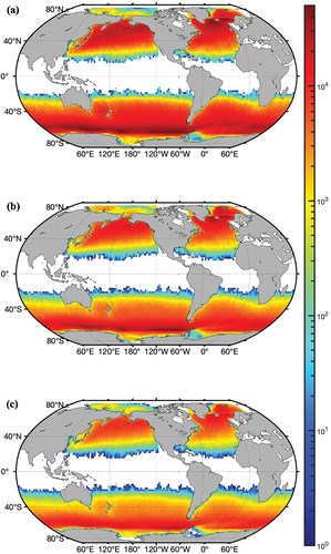
Figure 1. Sample sizes shown geographically for the number of (a) altimeter measurements of wind speed and $H_s$ within 500km of each storm center used in this study, (b) collocated pairs of wind speed measurements and ERA5 values on the 0.25${ }^o$ lat/lon grid, and (c) collocated pairs of $H_s$ measurements and ERA5 values on the 0.5${ }^o$ lat/lon grid. (a) is valid for either wind speed or $H_s$ measurements as they are stored at the same coordinates in the database.

In order to collocate the altimeter data to the ERA5 fields, a minimum of 5 altimeter data points are used, within a given radius around each ERA5 grid point, to calculate a linear distance weighted average which is then paired to the given ERA5 data point. A minimum of 5 data points is the same criteria used by Ribal and Young (2019) to stably compare altimeter data to buoy measurements. In the case of the ERA5 $|\mathit{U}10|$($H_s$) fields, we use a radius threshold of 25(50) km over which to collect and average altimeter data. Campos (2023) tested various methods of collocating altimeter wind and wave data to buoy measurements and found that using radii of 25 or 50 km showed almost identical bias, RMSE, scatter index, and correlation coefficients provided that an averaging method was utilized over a minimum number of data points opposed to a nearest neighbor comparison. Because the ERA5 $|\mathit{U}10|$ fields have a higher spatial resolution of 0.25${ }^o$ we choose a pairing radius of 25 km to avoid the overuse of the altimeter data that would occur with a larger radius. With the ERA5 $H_s$ fields having a coarser resolution of 0.5${ }^o$, a radius of 50 km is utilized for the collocation of wave data. The same threshold in time of plus or minus 0.5 hrs is used for all ERA5-altimeter data collocations, as suggested by Campos (2023) based on time lag autocorrelations from buoy measurements of $H_s$ and $|\mathit{U}10|$. Sample sizes of the altimeter data collected along EC tracks, the number of $|\mathit{U}10|$ ERA5-altimeter data collocations, and the number of $H_s$ ERA5-altimeter data collocations are shown geographically in Figure 1.

2.4. Characteristic Radius (R_L) and The EC centered reference frame

In order to account for varying EC size when performing the composite analyses over many different ECs, we have defined a characteristic radii using the same fields of the Laplace of MSLP as were used for the EC detection algorithm in Lodise et al. (2022). Collins et al. (2021) normalized tropical cyclone size based on the cyclone radius of max winds; however, initial investigation here showed the radius of max wind is not a well behaved feature of ECs due their lack of radial symmetry related to the evolution of fronts, and corresponding wind jets, present in these storms. Instead, we define a radius, $R_L$, as the minimum distance in kilometers from the EC center to the nearest zero contour in the Laplace of MSLP field, or in other words, the nearest inflection point in the MSLP field. S1 shows an animation of EC tracks with circles of corresponding radii length $R_L$.

After the ERA5-altimeter data collocation is completed within 500 km of each EC center, the data are converted from its original latitude/longitude grid to a storm centered reference frame by defining each EC center as the origin in the new coordinate system at every hourly time step. Latitude and longitude coordinates are then converted into units of kilometers in x and y from the origin. The data are then rotated, again at each time step, such that the direction of EC movement toward the next data point along the storm track is pointed up the page. The x and y coordinates of the data, now in kilometers, are then normalized by the corresponding time step’s $R_L$ before being binned and averaged in x and y.

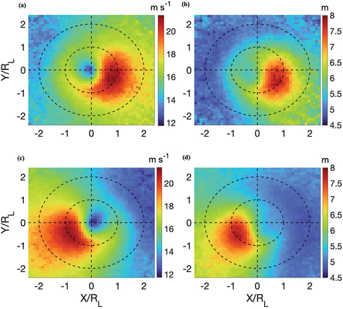
Average composites of $|\mathit{U}10|$ and $H_s$ in the EC reference frame from only altimeter data for all ECs in the Northern and Southern Hemisphere are shown in Figure 2(a–d), respectively. Two concentric circles outlining 1$R_L$ and 2$R_L$ are also included in each plot. Also shown in Figure 2b is the labeling convention of EC quadrants I-IV used through out the present work. Figure 3 shows the sample sizes for altimeter data and collocated pairs of altimeter data and ERA5 values, split by Northern and Southern Hemisphere for the same data as in Figure 1 shown in the storm centered reference frame.

Figure 2. Rotated and averaged composites of (a) wind speed and (b) $H_s$ from satellite altimeter observations for all ECs in the Northern Hemisphere. (c) and (d) show the same for the Southern Hemisphere, respectively. The position of all data around each storm center have been normalized by $R_L$ after being rotated to align all directions of EC movement up the page. (b) also shows the labeling convention of the four quadrants divided by the straight dotted lines. Again, the dotted circles depict radii of length $1R_L$ and $2R_L$. Bins are 0.1 $R_L$ wide in X and Y.

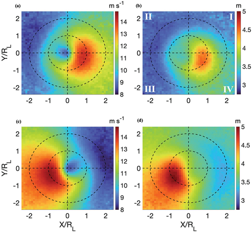
Figure 3. Number of $H_s$ altimeter observations (identical for $|\mathit{U}10|$ observations) shown in the normalized EC reference frame for the (a) Northern and (b)Southern Hemisphere. (c,d) the number of collocated ERA5 and $|\mathit{U}10|$ observations in Northern and Southern Hemisphere ECs, respectively. (e) and (f) show the same for collocated pairs of $H_s$. Bins are 0.1 $R_L$ wide in X and Y.

2.5. Evaluation of ERA5

After the collocation and conversion of coordinates into the EC reference frame, we calculate the Root Mean Squared Error (RMSE),

(1) $\mathit{RMSE}=\sqrt{\frac{1}{n}\sum _{\mathit{i}=1}^n{(X_{mo{d}_i}-X_{ob{s}_i})}^2}$(1)

and Percent Bias,

(2) $\%\mathit{Bias}=\frac{100}{n}\sum _{\mathit{i}=1}^n\frac{(X_{mo{d}_i}-X_{ob{s}_i})}{X_{ob{s}_i}},$(2)

where $X_{mo{d}_i}$ and $X_{ob{s}_i}$ are the collocated pairs of ERA5 and altimeter data, respectively, and $\mathit{n}$ is the sample size within individual spatial bins (as shown in Figure 2). The choice of skill metrics used here is meant to give a sense of absolute error (RMSE) as well as relative (Percent Bias) error with respect to varying wind and wave height magnitudes. The variance of the collocated ERA5 and altimeter data are also calculated in each spatial bin as

(3) $\mathit{Va}{r}_{\mathit{mod},\mathit{obs}}=\frac{1}{\mathit{n}-1}\sum _{\mathit{i}=1}^n|X_{mo{d}_i,\mathit{ob}{s}_i}-{\mu }_{\mathit{mod},\mathit{obs}}{|}^2,$(3)

where $\mathit{\mu }$ is the mean within each bin, and compared through out the analysis to provide further insight into model performance.

3. Results

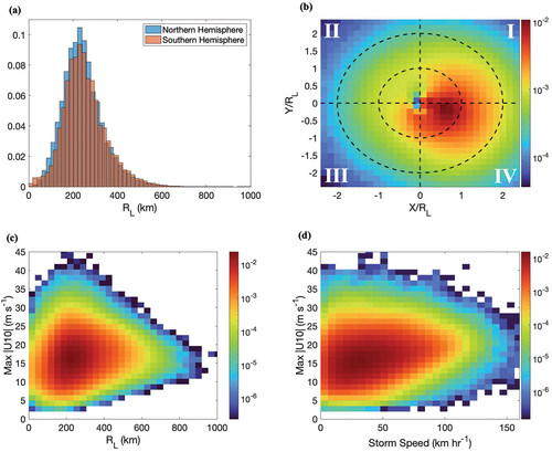
Relative probability histograms of $R_L$, calculated at every time step along each EC storm track can be found in Figure 4a. Figure 4b shows the relative probability map of the maximum wind speed location, defined from the ERA5 wind field within 500 km of each EC center, from all the ECs used in this study in the rotated and normalized coordinate system. The relationship between $R_L$ and EC intensity, defined by the maximum $|\mathit{U}10|$ sampled from ERA5 within each EC, can also be seen in the joint probability histogram in Figure 4c. As shown in this figure, ECs with the highest maximum winds do not occur at the largest values of $R_L$, but instead show peak maximum winds at $R_L\sim$ 200 km. Figure 4d shows the joint relative probability distribution of the ERA5 defined max $|\mathit{U}10|$ and EC storm speed from each time step along all EC trajectories.

Figure 4. (a) relative probability histograms of $R_L$, defined as the minimum distance from each EC center to the zero contour in the Laplace of the MSLP field, for the Northern and Southern Hemisphere. (b) relative probability histogram of the maximum wind speed location, defined using the ERA5 U10 wind fields within 500km of each storm center, normalized by each storm’s $R_L$ for all ECs. Note: Southern Hemisphere data has been flipped about the y-axis to match Northern Hemisphere cyclone orientation. Coordinates have been rotated before binning to align all EC directions up the page. Also shown is the labeling convention of the four EC quadrants separated by the straight dotted lines. The two dotted line circles depict $1R_L$ and $2R_L$ radii. (c) joint relative probability histogram of maximum wind speed and characteristic radius $R_L$. (d) joint relative probability histogram of maximum wind speed and EC translational speed. Data are collected from every hourly time step along all EC trajectories for each plot.

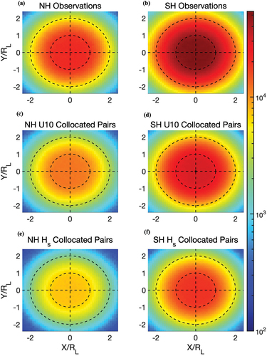
In order to explore extreme values of $|\mathit{U}10|$ and $H_s$ within ECs, we plot the 90${ }^{\mathit{th}}$ percentile of the altimeter measurements within each spatial bin in the rotated storm centered reference frame for each hemisphere in Figure 5. Figure 2 shows that while on average the Southern Hemisphere is home to more intense ECs, having higher winds and larger wave heights than observed in the Northern Hemisphere; Figure 5 reveals that the extreme values of these measurements are of very similar magnitude in each hemisphere. The organization of $|\mathit{U}10|$ and $H_s$ in Figures 2 and 5 shows the largest wind speeds and wave heights in the Northern Hemisphere to occur in quadrant IV on, or just inside $1R_L$. Also seen in quadrant III for the Northern Hemisphere case is a region of increased $|\mathit{U}10|$ and $H_s$ along $1R_L$, apparent in both the average and 90^th percentile composite figures. This suggests the normalization using $R_L$ is useful in aligning the structure of the core winds and subsequent waves being observed in the ECs. Similarly, the region of the largest $|\mathit{U}10|$ and $H_s$ in quadrants I and IV for the Northern Hemisphere are contained by the circle depicting $2R_L$, showing the spatial extent of the most impactful, extreme conditions in ECs on average. The Southern Hemisphere composites (Figures 2c, d) mirror the same features seen in the Northern Hemisphere about the y-axis, consistent with the clockwise wind circulation observed in ECs in the Southern Hemisphere due to the change in sign of the Coriolis force across the equator. This wind pattern results in the alignment of wind and EC translational velocities on the left side of ECs (quadrants II and III) relative to the storm center direction of motion.

Figure 5. $90\mathit{th}$ percentile composites of (a) wind speed and (b) $H_s$ from satellite altimeter observations for all ECs in the Northern Hemisphere. (c) and (d) show the same for all the ECs in the Southern Hemisphere. Bins are 0.1 $R_L$ wide in X and Y.

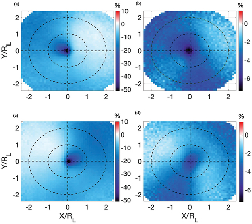
The RMSE and percent bias calculated using all the $|\mathit{U}10|$ and $H_s$ collocated pairs for the Northern and Southern Hemispheres data sets are shown in Figures 6 and 7, respectively. Figure 6(a, c) show that the reanalysis struggles to correctly represent wind speeds at EC centers, and Figure 7(a, c) reveal that the reanalysis is underestimating the relatively mild winds observed at this location by up to $\sim$50%. The underestimation of $|\mathit{U}10|$ is also shown to radiate out predominately into quadrant II in the Northern Hemisphere and quadrant I in the Southern Hemisphere, again exemplifying the symmetry between ECs on either side of the equator. This symmetry is also seen in the statistical metrics for $H_s$(Figures 6b, d and 7b, d). The reanalysis is found to underestimate $H_s$ within 1 $R_L$ with the worst performance occurring within EC centers, again with this bias radiating out from the center into quadrants II and IV(I and III) in the Northern(Southern) Hemisphere, as highlighted in Figures 7(b, d). Interestingly, the $H_s$ underestimation seen in the EC centers is notably more significant in the Northern Hemisphere. Figure 6 also shows the reanalysis to have RMSE values greater than $\sim$0.5 m within 1 $R_L$ of EC centers in three out of four quadrants in the Northern Hemisphere, while this region of high RMSE is contained mostly to quadrant III in the Southern Hemisphere.

Figure 6. RMSE (Equation 1(1) $\mathit{RMSE}=\sqrt{\frac{1}{n}\sum _{\mathit{i}=1}^n{(X_{mo{d}_i}-X_{ob{s}_i})}^2}$(1) ) computed using collocated pairs of ERA5 and satellite altimeter measurements of (a) $|\mathit{U}10|$ and (b) $H_s$ in the Northern Hemisphere. (c) and (d) show the RMSE calculated in Southern Hemisphere ECs. Bins with less than 500 data points have been omitted in each plot. Bins are 0.1 $R_L$ wide in X and Y.

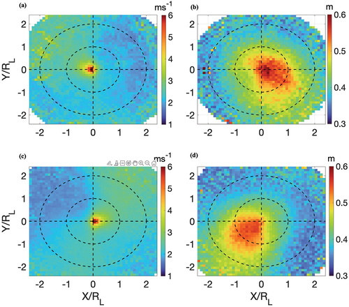
Figure 7. Percent bias, calculated as shown in Equation 2(2) $\%\mathit{Bias}=\frac{100}{n}\sum _{\mathit{i}=1}^n\frac{(X_{mo{d}_i}-X_{ob{s}_i})}{X_{ob{s}_i}},$(2) , in Northern Hemisphere ECs for ERA5 (a) $|\mathit{U}10|$ and (b) $H_s$. The same for South Hemisphere ECs is shown in (c) and (d), respectively. Bins are 0.1 $R_L$ wide in X and Y. Bins with less than 500 data points have been omitted in each plot.

Altimeter measurement of $|\mathit{U}10|$ and $H_s$ are further divided based on varying maximum wind speed, defined using the ERA5 wind fields as in Figure 4b, and translational storm speed calculated along each storm track. The average composites of $|\mathit{U}10|$ and $H_s$ from the original (non-collocated) altimeter data set in the Northern Hemisphere can be found in Figures 8 and 9, respectively. In each row of Figure 8, we observe an increase in $|\mathit{U}10|$ in quadrants I and IV, while quadrants II and III show a steady to slight decrease in wind magnitudes on average as storm speed increases. This illustrates that as ECs start to move faster the the EC velocity starts to overcome the cyclonic circulation around the EC center, resulting in lower wind speeds on the left side of the storms, where storm velocity and winds oppose one another, and higher wind speeds on the right side of storms where they align. When EC velocities are small ($<$20 km hr⁻¹), the wind fields are much more uniform across the four quadrants with only a slight increase in $|\mathit{U}10|$ seen in quadrants I and IV. As the composite analysis does not resolve the highly variable nature of EC wind fields in time as their frontal dynamics develop, this does not suggest that any particular snap shot of a slow moving EC wind field will be this uniform, but only that there is no preferential region for increased wind speeds.

Figure 8. Composites of rotated and averaged $|\mathit{U}10|$ measured by satellite radar altimeter, binned by increasing maximum wind speed (MaWi) and translational EC storm speed (StSp) for ECs in the Northern Hemisphere. Bins are 0.2$R_L$ wide in X and Y. Bins with less than 100 data points have been omitted.

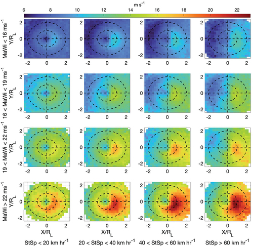
Figure 9. Composites of rotated and averaged $H_s$ measured by satellite radar altimeter, binned by increasing maximum wind speed (MaWi) and translational EC storm speed (StSp) for ECs in the Northern Hemisphere. Bins with less than 100 data points have been omitted.

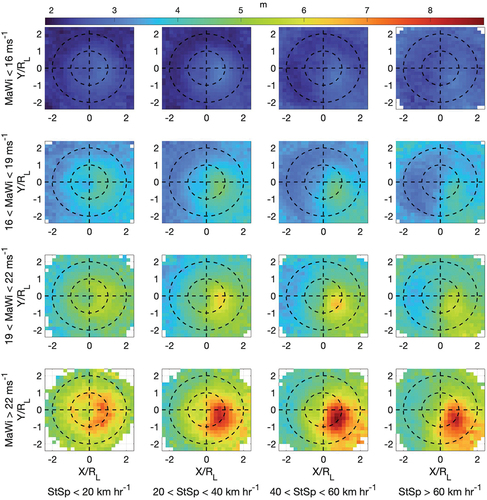
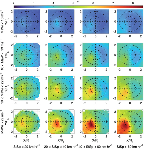
Figure 9 shows the corresponding composite plots of $H_s$ over the same maximum wind and storm speed bins. We observe wave heights which increase with maximum winds and also increase and organize spatially (on the right side of the ECs mostly in quadrant IV) with increasing storm speed, but unlike the $|\mathit{U}10|$ composites, we do not observe the largest $H_s$ in the fastest moving ECs. For ECs with maximum wind speeds above 19 m s⁻¹, the largest averages of $H_s$ are associated with ECs traveling between 40 and 60 km hr⁻¹. Weaker ECs with max winds $<$ 19 m s⁻¹ show less variation with storm speed, but still show a slight increase in average $H_s$ for storm speeds from 20–60 km hr⁻¹. Average maximum wave heights are found very near 1 $R_L$ across all the varying storm conditions, usually in quadrant IV, with the exception being the slowest moving ECs which show less preferential wave growth by quadrant. Figures 10 and 11 show almost perfectly mirrored trends for $|\mathit{U}10|$ and $H_s$ in Southern Hemisphere ECs of varying storm speed and max wind.

Figure 10. Same as Figure 8 for Southern Hemisphere EC $|\mathit{U}10|$ observations.

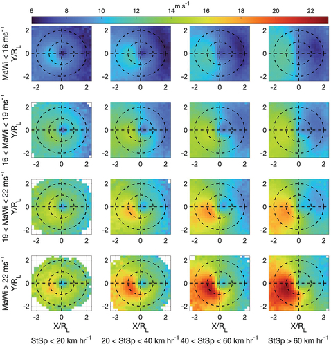
Figure 11. Same as Figure 9 for Southern Hemisphere EC $H_s$ observations.

For brevity, the remainder of the figures (Figures 12–21) shown here are created using a combined data set consisting of all the Northern and Southern Hemisphere data, made possible by multiplying the x-coordinates of the Southern Hemisphere storm data by a factor of (−1) in order to transfer the data into the equivalent Northern Hemisphere storm centered convention. After all the EC data are combined, we then explore the variance, RMSE, and percent bias of the quantities of interest over the same varying EC conditions.

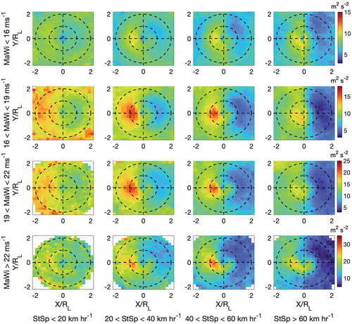
Figure 12. Variance of $|\mathit{U}10|$ observations calculated in each spatial bin across the same ranges of max wind speed and storm speed as in Figure 8. The values resulting from the collocation to the ERA5 grid are used to calculate the values shown. Note changing color bar limits for each row. For this figure and subsequent figures, all Southern Hemisphere EC data has been flipped about the y-axis, placing the data in a Northern Hemisphere EC reference frame, and combined with the Northern Hemisphere data sets.

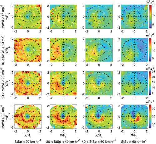
Figure 12 and 13 show the variance of $|\mathit{U}10|$ calculated using the collocated pairs of altimeter data and ERA5 values, respectively, to accurately asses the reanalysis based on the observations across varying storm characteristics. Unsurprisingly, we find more variance overall in the observations across all the max wind/storm speed defined bins; however, there are some qualitative similarities between the two data sets. Again we see an organization of structures as storm speeds begin to increase across all the max wind bins in both the model and observations. The most striking feature is the band of high variance which spans quadrants II-IV and wraps into the inner radius of $1R_L$ that can be seen across many of the plots in both figures, although substantially more intense in the observations. The variance of the wind speeds on the right side of ECs (quadrants I and IV) is not well represented by the model when compared to the observations.

Figure 13. Variance of $|\mathit{U}10|$ from ERA5 fields calculated in each spatial bin across the same ranges of max wind speed and storm speed as in Figure 8. Values used are the same as those paired with the observational data.

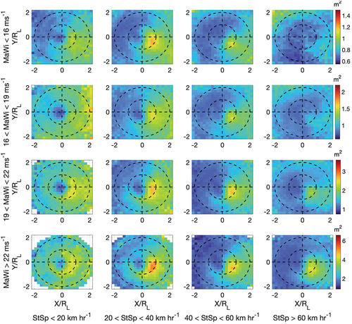
Similarly, the variance of $H_s$ within each spatial bin across varying EC conditions from ERA5 and the collocated altimeter observations are shown in Figures 14 and 15. Again, the variance seen in the reanalysis wave heights are qualitatively similar to that derived from the observations with both showing high variance on the right side of ECs with the largest values in the fourth quadrant. This region also corresponds to the largest wave heights seen in Figures 9 and 11. Although not as strong as seen in the wind variance, we do see a corresponding band of high variance in $H_s$ along $1R_L$ on the left and back side (III and IV) of ECs from both model and observations. However, the variance seen in quadrant II of the wind speed is not reflected in the $H_s$ figures, which suggests the opposing winds and storm direction in this quadrant do not facilitate wave growth as effectively.

Figure 14. Variance of $H_s$ observations, using the values collocated with ERA5, across the given ranges of max wind speed and storm speed.

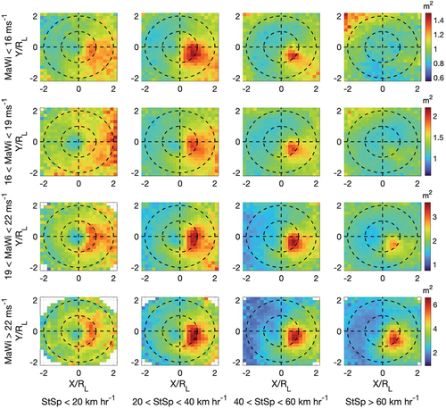
Figure 15. Variance of ERA5 $H_s$ across ranges of max wind speed and storm speed shown.

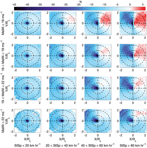
Figures 16 and 17 show the RMSE and percent bias over the same max wind/storm speed intervals calculated from collocated pairs of $|\mathit{U}10|$ within each spatial bin of the EC reference frame. Across all the varying EC conditions explored, the ERA5 struggles to accurately represent the moderate wind speeds observed at EC centers resulting in RMSE values up over 6 m s⁻¹ and percent bias values showing underestimation of wind speed by 45%. Overall wind speeds are underestimated within ECs, with the small exception of some positive percent bias on the order of 1–5% in quadrant I of fast moving relatively weaker storms. Figure 17 shows that in terms of percent bias of $|\mathit{U}10|$, quadrant II is systematically underestimated more than any other cyclone region, while Figure 16 shows that in more intense ECs large RMSE can also be found quadrant IV where the largest wind speeds occur. Best shown in the row of increasing storm speed for ECs with max winds $>$ 22 m s⁻¹, Figure 16 shows how errors become organized as storm speed increases, with quadrants II and IV showing the highest values of RMSE, outside the very center of ECs.

Figure 16. RMSE of $|\mathit{U}10|$ calculated in each spatial bin over the given ranges of max wind and storm speed.

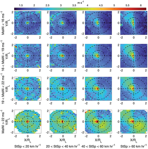
Figure 17. Same as Figure 16 showing percent bias of ERA5 $|\mathit{U}10|$.

The same statistical metrics for $H_s$ are presented over the given EC max wind and storm speed intervals in Figures 18 and 19. The largest RMSE values found within the given ranges of ECs are located in quadrant IV during fast moving EC of strong intensity. Across each row, as storm speed increases, we find the largest RMSE values to again organize onto the right (I and IV) side of ECs. There also exists a backward drift of the largest observed errors from quadrant I to IV as storm speed increases, likely because ECs with these velocities are moving faster than the waves being produced underneath. This is also apparent in the largest values of average $H_s$ shown in Figures 9 and 11. Similar to average $H_s$, the largest RMSE values are not associated with the fastest moving ECs, where the strongest winds are typically found as shown in Figures 8 and 10.

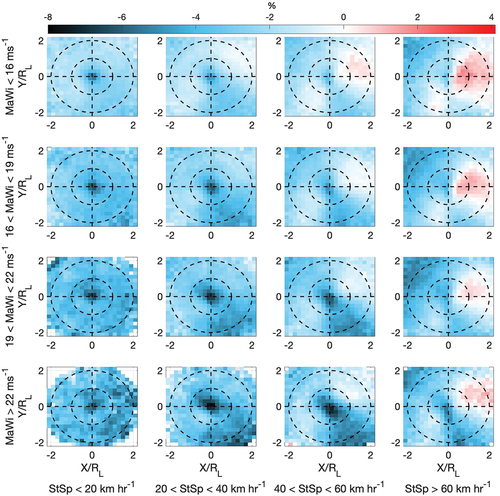
Figure 19 shows the percent bias trends of $H_s$ to be very similar to that of $|\mathit{U}10|$ shown in Figure 17, including the strongest underestimation of wave heights residing in EC centers and the slight over estimation of wave heights on the right side of fast moving, mostly weaker storms. We also see a similar organization of percent bias of $H_s$ with increasing storm speed; however, unlike with $|\mathit{U}10|$, the largest percent bias is found in quadrant IV and storm centers, while the large percent wind bias in quadrant II is not reflected in the $H_s$ bias proportionately.

Figure 18. RMSE of $H_s$ calculated in each spatial bin over the given ranges of max wind and storm speed.

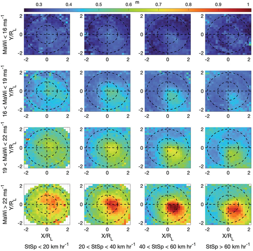
Figure 19. Percent bias of $H_s$ calculated in each spatial bin over the given ranges of max wind and storm speed.

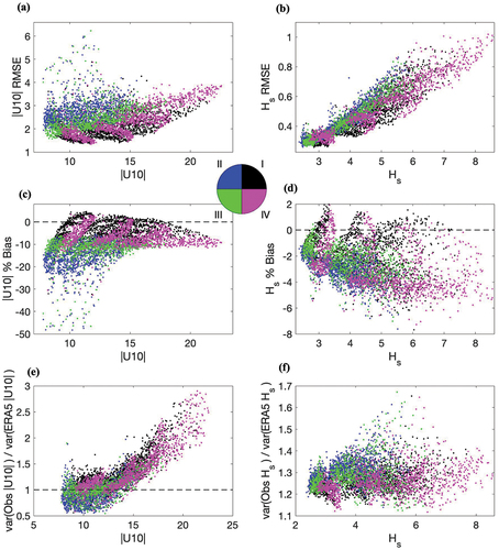
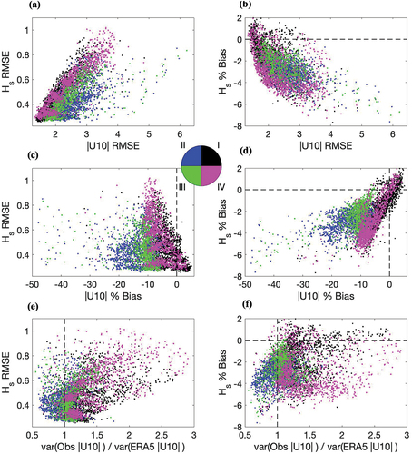
All the spatial bin values within $2R_L$ of the EC reference frame origin from Figures 12–19 are plotted against the corresponding bin averages of $H_s$ and $|\mathit{U}10|$, calculated from the collocated altimeter data from both hemispheres in Figure 20. It is clear that from the scatter plot shown that each quadrant has distinct statistical characteristics, with a very clear regime change between the left (II and III) and right side quadrants (I and IV). Figure 20(a, c) show outliers of $|\mathit{U}10|$ RMSE and percent bias which are associated with the EC center, showing up predominately in quadrants II and III. These quadrants also perform worse in general compared to quadrants I and IV where ERA5 has the most skill however the $|\mathit{U}10|$ associated plots show this skill to decrease in more intense ECs. Figure 20b similarly shows ERA5 to have more skill representing $H_s$ in quadrants I and IV, evident by the decreased slope of the scatter with increasing $H_s$. This skill too, degrades with increasing $H_s$ measurements. Figure 20d shows that in terms of percent bias, quadrant IV predominately shows the least skill as wave heights increase while interestingly quadrant I shows a slightly different behavior having more values much closer to zero. The ERA5 reanalysis seems to adequately represent the wind variance in quadrant III, while showing more variance than seen in the observations in quadrant II. The variance observed for the same in quadrants I and IV reach more than 2.5× that of the reanalysis at higher wind speeds (Figure 20e). The ratio between the variance of $H_s$ from observations and the model is relatively constant across all quadrants and wave height magnitudes (Figure 20f).

Figure 20. Scatter plots of the bin values shown in Figures 12–19 plotted against average wind speed(a,c,e) and $H_s$(b,d,f) from all ECs in each corresponding spatial bin, colored by EC quadrant, as depicted by the circle shaped legend. Values outside a radius of $2R_L$ are excluded from the scatter plots. Average $|\mathit{U}10|$ and $H_s$ values are calculated using all EC data from both hemispheres.

Figure 21 shows the same data as seen in Figure 21 however we now compare errors in the wind forcing $|\mathit{U}10|$ to errors in the $H_s$. Again, we see a clear separation of data pairs sampled from the right or left side of the EC reference frame. Figures 21(a, b) show that errors in the wind forcing result in more drastic $H_s$ error in quadrants I and IV, where wind and storm direction align. The same can be seen in Figures 21(c, d). Figure 21e shows that under represented variance in the model winds are associated with higher values of $H_s$ RMSE on the right side quadrants; however, Figure 21f shows that in terms of percent bias, the fourth quadrant shows greater underestimation of $H_s$ than in quadrant I. It should be noted that the clustering of data points seen in several of the panels in Figures 20 and 21 are due to the previous binning by maximum wind speed.

Figure 21. Scatter plots of the bin values shown in Figures 12–19 colored by EC quadrant, as depicted by the circle shaped legend. Values outside a radius of $2R_L$ are excluded from the scatter plots.

4. Discussion

Being defined as the minimum distance to an inflection point in the MSLP field, one can think of $R_L$ as a definable core with symmetric structure within the larger, typically asymmetric ECs. The distribution of $R_L$ in Figure 4a reveals this quantity to be remarkably similar for Northern and Southern Hemisphere ECs, suggesting radii size of ECs in the two regions are constrained, to a large degree, by the same dynamics. Schneidereit, Blender, and Fraedrich (2010) calculated EC radii based on a Gaussian fitting method to the 1000 hPa geopotential height and found similar shaped distribution of radii centered at $\sim$300–400 km. Comparing these distributions to the distribution of $R_L$ here, it can be inferred that our characteristic radii based on the nearest inflection point in the MSLP field is typically on the order of $\sim \frac{2}{3}$ to $\frac{3}{4}$ the radii found by Schneidereit, Blender, and Fraedrich (2010). Although we use a constant radius threshold of 500 km to perform the pairing of data to EC centers, preliminary investigations showed that varying this radius of altimeter data collection up to 2.5$R_L$ at each time step, did not affect the composite averages for a 10-year subset of ECs. Therefore we chose to keep the constant radius of 500 km in order to make accurate comparisons to previous studies (Ponce de León and Bettencourt 2021) and to minimize computational resources needed.

Comparing Figure 2a, b to results from Ponce de León and Bettencourt (2021), which presented similar composite figures using altimeter data in the North Atlantic, it is clear that the rotation based on storm direction and spatial normalization using $R_L$ has organizing effects on the final composite averages. This is evident by the concentration of the highest winds and largest wave heights into smaller relative areas confined to the right side of the EC coordinate system and higher average values of both variables. The composite figures shown here also show increased alignment of the strongest winds and highest wave heights, while also revealing more drastic changes from quadrant to quadrant. Figures 6 and 7 also highlight the organization of bias and RMSE in the reference frame used here, leading to higher error metrics regionally. When calculating RMSE of ERA5 winds geographically, Campos et al. (2022) showed maximum values of less that 2 m s⁻¹ in the extratropical region, while here we show the RMSE of winds at the center of the EC reference frame are a factor of 3 larger (Figure 6). It should be noted that the large error seen in the center of the cyclones could be the result of slight cyclone location offsets between the ERA5 fields and the observations. Figure 16 also shows RMSE values up to 4 m s⁻¹ in quadrant IV of intense ECs, showing that geographical averaging may have significant smoothing effects for these performance metrics.

Interestingly, Figures 6 and 7 show the ERA5 reanalysis performs worse in the Northern Hemisphere than in the Southern Hemisphere. This is most clearly seen in the RMSE and bias plots for $H_s$ near the center of storm reference frame in quadrants I and II and also in the noisier nature of the RMSE of both $|\mathit{U}10|$ and $H_s$. During their analysis of ERA5 winds using satellite derived wind data, Campos et al. (2022) also found the Southern Hemisphere to be better represented. Campos et al. (2022) investigated ERA5 performance under cyclonic wind conditions in the North and South Atlantic, finding the footprint of the gulf stream to be a site of strong underestimation of wind speeds. Gramcianinov, Hodges, and Camargo (2019) also showed this area to be a dominate sight of extratropical cyclogenesis, induced by the strong temperature gradients created by the warm water, western boundary current. This suggests that the stronger western boundary currents in the Northern Hemisphere, the Gulf Stream and the Kuroshio, both of which are regions of strong EC activity induced by strong latitudinal temperature and moisture gradients, is the cause of increased difficulty when modeling EC winds and waves in the Northern Hemisphere (Lodise et al. 2022). Wave-current interactions within strong western boundary currents have also been linked to underestimation of $H_s$ of up to 1–2 m (Ardhuin et al. 2017; Marechal and Ardhuin 2021).

The normalization using $R_L$ also highlights structural components of ECs. Figure 4b shows the organization of maximum wind locations, taken from ERA5 at each time step, to within 1 $R_L$ of storm centers, predominately on the right side quadrants. A region of high winds in quadrant III, likely linked to the advancing cold front, is also highlighted on the backside of the advancing ECs (see Ponce de León and Bettencourt (2021) for schematic). This cold jet of strong winds is also well illustrated by Figure 12, as it is likely responsible for the wind variability observed in quadrants I-III, which aligns itself with the $R_L$ radius. Although quite rare, needing very specific atmospheric conditions to occur, the formation of very intense sting jets in a small subset of storms could add to this signature in the variability, however the extent to which sting jets occur in these cyclones is difficult to infer and requires further investigation (Browning 2004; Hewson and Neu 2015). The frontal dynamics of ECs as cold fronts advance under warm air masses forcing convection and storm activity and the eventual occluding of the warm and cold front are likely other sources of variability in the observation of $|\mathit{U}10|$. Certain dynamical trends can also be linked to different developmental stages of ECs (i.e. cyclogenesis, intensification, maturity, and weakening). For the purpose of brevity, we have not applied methods to group life cycle stages in our analysis; however, we indirectly capture these stages, to some extend, by parsing the cyclone analysis by storm speed and maximum winds.

The effects of storm speed on wave growth is apparent in Figures 8–11. The strongest winds are found within the fastest moving ECs, however the largest wave heights in both hemispheres are found in the most intense ECs moving between 40 and 60 km hr⁻¹. Deep water waves with group speeds within this range of velocities correspond to wave periods of $\sim$14-21s and wavelengths of approximately 300–700 m, which are among the largest waves expected and previously observed within ECs (Hanafin et al. 2012; Siyahi et al. 2023). This suggests that the phenomena of dynamic or extended fetch, which describes the increased exposure of wind forcing due to the resonance between ECs and surface gravity waves traveling at the same velocity, is leading to increased wave heights at these speeds. It is of note that we also observe some of the highest variance of $H_s$ at these storm speeds as well (Figure 14), suggesting that storm speed is not enough to guarantee resonant effects between wind forcing and wave growth. The extent of wave growth preceding the occurrence of these storm velocities and the relative direction of storm motion to the direction of wave propagation are also key factors to consider. Additionally, Figure 14 shows similar variance of $H_s$ to that seen for $|\mathit{U}10|$ around $R_L$ in quadrants II and III but to a lesser extent than $|\mathit{U}10|$, likely due to opposing winds and EC velocity inhibiting wave growth in these storm regions.

The fastest moving ECs across all the max wind bins, traveling faster than this upper limit of group wave speed ($\sim$60 km hr⁻¹), effectively outrun the waves generated underneath, resulting in comparatively smaller waves heights than slower moving storms of the same intensity. The fastest moving storms, the range of which can be seen in Figure 4d, traveling over 100 km hr⁻¹ can also be traveling too quickly over the ocean surface for the sea state to become fully developed (Hell, Ayet, and Chapron 2021; Young and Vinoth 2013). Siyahi et al. (2023) showed that for two fast moving ECs, traveling at or above 60 km hr⁻¹, developing waves, which dominate the EC region, actually move backwards relative to the EC center and exit the storms in the rear, trailing behind the storms’ movements.

The performance of the ERA5 is also affected by the different dynamics at play on the right side (I and IV) versus the left side (II and III) of ECs (in a Northern Hemisphere reference frame). Figure 20 shows the performance of the reanalysis winds is highly dependent on EC region across RMSE, percent bias, and ratio of variance in the observation to that in the reanalysis. Although the largest errors in wind speeds are seen in the 2nd and 3rd quadrants (as seen in Figure 20a, c), Figure 21a-d shows the largest errors in $H_s$ are linked to the more moderate $|\mathit{U}10|$ errors seen at high wind speeds in quadrants I and IV. Figure 21 shows that smaller errors in the wind forcing in quadrants I and IV result in larger RMSE and underestimation in $H_s$ in the same quadrants. This added sensitivity in these EC regions could be explained again by the dynamic fetch phenomena. Underestimations in the wind forcing are effectively compounded as ECs travel at the same speed as the large waves being generated underneath, leading to the increased underestimation of wave heights. In quadrants II and III however, larger errors in wind forcing result in comparatively smaller errors in the wave field, which is congruous to the less active wave growth in these EC regions. During ECs where dynamic fetch was suspected to play an important role, numerical wave models have been shown to improve when corrected wind fields which better represent the extreme forcing are used (Hanafin et al. 2012).

The outliers seen in Figures 21a-d, corresponding to the large errors seen in the center of ECs for wind speeds and wave heights, is indicative that there is strong forcing close to the storm center that is not being accurately represented in the reanalysis. This is likely due to difficulties resolving the strong gradients in the wind field on the 0.25${ }^o$ grid. While this issue is most apparent across the center of ECs, this is likely a common occurrence across all cyclone regions, especially during rapid intensification and amidst warm and cold jets. Using data from an array of moored wave buoys off the US east coast, Cardone et al. (1996) highlighted how extreme sea states, specifically those forced by highly variable surface winds (both in space and time) within ECs are most likely to be underestimated by wave models. While comparisons to data collected at buoy locations give a one dimensional view of the cumulative effects leading to wave model underestimation, the EC-centered analysis presented here offers a more precise evaluation of model performance, specifically with regards to wind forcing and wave height accuracy, and the relationship between the two in different EC regions.

5. Conclusion

Using altimeter measurements of $H_s$ and $\mathit{U}10$ in an EC centered reference frame, we have evaluated the performance of the widely used and state-of-the-art ECMWF ERA5 reanalysis under a variety of EC conditions. Rotating the reference frame of data to align all EC velocities and employing a new spatial normalization based on a characteristic radius of ECs highlights structures not previously observed in altimeter based composite analyses. The coordinate frame used also emphasizes the dependence of the reanalysis performance on storm region, clearly displaying the added sensitivity of the wave field to wind forcing on the right side of ECs, with respect to their forward motion under the Northern Hemisphere convention used here.

The well-known problem of operational hindcasts missing the peak wave heights in extreme conditions is again apparent here. Based on our findings a significant source of error in the wave field is underestimation of the wind forcing, especially near the strong gradients of wind speed close to the storm centers of ECs. The wind speeds and wave heights at the center of ECs are shown to be systematically underestimated across most of the EC conditions investigated here, resulting in biases of up 45% and 8% for $|\mathit{U}10|$ and $H_s$, respectively. The percent bias associated with the largest wave heights and largest wind speeds reach upwards of 6% and 10%, respectively. The highest RMSE values of $H_s$, which reach upwards of 1 m, are predominately located in quadrant IV of the most extreme storms, extending out from the storm center in each composite. Errors of this magnitude at extreme wave generation sites are substantial when considering maritime hazards and create more difficulty when trying to model and understand related problems including wave energy propagation, wave run up, and coastal erosion.

Acknowledgments

The authors would like to acknowledge Darren Wright and Randolph Bucciarelli from the Coastal Data Information Program (CDIP) who facilitated the use of computational resources needed to analyze the large data sets used here.

Disclosure statement

No potential conflict of interest was reported by the author(s).

Data availability statement

The ERA5 reanalysis is available directly from the Copernicus Climate Change Service (C3S) Climate Date Store (https://cds.climate.copernicus.eu/#!/search?text=ERA5&type=dataset). The Satellite Radar Altimeter data can be accessed through the ongoing IMOS (Integrated Marine Observing System) Surface Waves Sub-Facility Altimeter Wave/Wind database which is available through the Australian Ocean Data Network portal (AODN: https://portal.aodn.org.au/). The cyclone track position data used to produce the figures here can be found at https://github.com/jlodise/JGR2022_ExtratropicalCycloneTracker.

Supplementary material

Supplemental data for this article can be accessed online at https://doi.org/10.1080/21664250.2023.2301181

Additional information

Funding

This work was supported by a United Sates Army Corps of Engineers Grant (W912HZ1920020) through the Integrative Oceanography Division at The Scripps Institution of Oceanography. Dr. Clarence Collins was supported by The United Sates Army Corps of Engineers Civil Works under the Coastal Ocean Data Systems (CODS) program managed by Dr. Spicer Bak and Dr. Julie Rosati and by the Office of Naval Research Littoral Geosciences and Optics program managed by Dr. Reggie Beach.

References

- Abdalla, Saleh, Peter A.E.M. Janssen, and Jean Raymond Bidlot. 2010. “Jason-2 OGDR Wind and Wave Products: Monitoring, Validation and Assimilation.” Marine Geodesy 33 (sup1): 239–255. https://doi.org/10.1080/01490419.2010.487798.
- Alves, Jose Henrique G.M., and Ian R. Young. 2003. “On Estimating Extreme Wave Heights Using Combined Geosat, Topex/Poseidon and ERS-1 Altimeter Data.” Applied Ocean Research 25 (4): 167–186. https://doi.org/10.1016/j.apor.2004.01.002.
- Ardhuin, F., S. T. Gille, D. Menemenlis, C. B. Rocha, N. Rascle, B. Chapron, J. Gula, and J. Molemaker. 2017. “Small-Scale Open Ocean Currents Have Large Effects on Wind Wave Heights.” Journal of Geophysical Research Oceans 122 (6): 4500–4517. https://doi.org/10.1002/2016JC012413.
- Bell, R. J., S. L. Gray, and O. P. Jones. 2017. “North Atlantic Storm Driving of Extreme Wave Heights in the North Sea.” Journal of Geophysical Research Oceans 122 (4): 3253–3268. https://doi.org/10.1002/2016JC012501.
- Browning, K. A. 2004. “The Sting at the End of the Tail: Damaging Winds Associated with Extratropical Cyclones.” Quarterly Journal of the Royal Meteorological Society 130 (597): 375–399. https://doi.org/10.1256/qj.02.143.
- Campos, R. M. 2023. “Analysis of Spatial and Temporal Criteria for Altimeter Collocation of Significant Wave Height and Wind Speed Data in Deep Waters.” Remote Sensing 15 (8): 2203. https://doi.org/10.3390/rs15082203.
- Campos, Ricardo M., Carolina B. Gramcianinov, Ricardo de Camargo, and Pedro L. da Silva Dias. 2022. “Assessment and Calibration of ERA5 Severe Winds in the Atlantic Ocean Using Satellite Data.” Remote Sensing 14 (19): 4918. https://doi.org/10.3390/rs14194918.
- Cardone, V. J., R. E. Jensen, D. T. Resio, V. R. Swail, and A. T. Cox. 1996. “Evaluation of Contemporary Ocean Wave Models in Rare Extreme Events: The ‘Halloween storm’ of October 1991 and the ‘Storm of the century’ of March 1993.” Journal of Atmospheric and Oceanic Technology 13 (1): 198–230. https://doi.org/10.1175/1520-0426(1996)013<0198:EOCOWM>2.0.CO;2.
- Cavaleri, Luigi. 2009. “Wave Modeling—Missing the Peaks.” Journal of Physical Oceanography 39 (11): 2757–2778. https://doi.org/10.1175/2009JPO4067.1.
- Collins, Clarence, and Tyler Hesser. 2021. altWIZ: A System for Satellite Radar Altimeter Evaluation of Modeled Wave Heights. Technical Report. Duck, NC, USA: US Army Engineer Research and Development Center.
- Collins, Clarence, Tyler Hesser, Peter Rogowski, and Sophia Merrifield. 2021. “Altimeter Observations of Tropical Cyclone-Generated Sea States: Spatial Analysis and Operational Hindcast Evaluation.” Journal of Marine Science and Engineering 9 (2): 1–31. https://doi.org/10.3390/jmse9020216.
- Gramcianinov, C. B., K. I. Hodges, and R. Camargo. 2019. “The Properties and Genesis Environments of South Atlantic Cyclones.” Climate Dynamics 53 (7–8): 4115–4140. https://doi.org/10.1007/s00382-019-04778-1.
- Hanafin, Jennifer A., Yves Quilfen, Fabrice Ardhuin, Joseph Sienkiewicz, Pierre Queffeulou, Mathias Obrebski, Bertrand Chapron, et al. 2012. “Phenomenal Sea States and Swell from a North Atlantic Storm in February 2011: A Comprehensive Analysis.” Bulletin of the American Meteorological Society 93 (12): 1825–1832. https://doi.org/10.1175/BAMS-D-11-00128.1.
- Hell, M. C., Alex Ayet, and Bertrand Chapron. 2021. “Swell Generation Under Extra-Tropical Storms.” Journal of Geophysical Research Oceans 126 (9). https://doi.org/10.1029/2021JC017637.
- Hersbach, Hans, Bill Bell, Paul Berrisford, Shoji Hirahara, András Horányi, Joaquín Muñoz-Sabater, Julien Nicolas, et al. 2020. “The ERA5 Global Reanalysis.” Quarterly Journal of the Royal Meteorological Society 146 (730): 1999–2049. https://doi.org/10.1002/qj.3803.
- Hewson, Tim D., and Urs Neu. 2015. “Cyclones, Windstorms and the IMILAST Project.” Tellus, Series A: Dynamic Meteorology and Oceanography 67 (1): 27128. https://doi.org/10.3402/tellusa.v67.27128.
- Hodges, Kevin, Alison Cobb, and Pier Luigi Vidale. 2017. “How Well are Tropical Cyclones Represented in Reanalysis Datasets?” Journal of Climate 30 (14): 5243–5264. https://doi.org/10.1175/JCLI-D-16-0557.1.
- Holliday, Naomi P., Margaret J. Yelland, Robin Pascal, Val R. Swail, Peter K. Taylor, Colin R. Griffiths, and Elizabeth Kent. 2006. “Were Extreme Waves in the Rockall Trough the Largest Ever Recorded?” Geophysical Research Letters 33 (5): 2–5. https://doi.org/10.1029/2005GL025238.
- Izaguirre, Cristina, Fernando J. Méndez, Melisa Menéndez, and Inigo J. Losada. 2011. “Global Extreme Wave Height Variability Based on Satellite Data.” Geophysical Research Letters 38 (10). https://doi.org/10.1029/2011GL047302.
- Kita, Yuki, Takuji Waseda, and Adrean Webb. 2018. “Development of Waves Under Explosive Cyclones in the Northwestern Pacific.” Ocean Dynamics 68 (10): 1403–1418. https://doi.org/10.1007/s10236-018-1195-z.
- Lodise, John, Sophia Merrifield, Clarence Collins, Peter Rogowski, James Behrens, and Eric Terrill. 2022. “Global Climatology of Extratropical Cyclones from a New Tracking Approach and Associated Wave Heights from Satellite Radar Altimeter.” Journal of Geophysical Research Oceans 127 (11). https://doi.org/10.1029/2022JC018925.
- Marechal, Gwendal, and Fabrice Ardhuin. 2021. “Surface Currents and Significant Wave Height Gradients: Matching Numerical Models and High-Resolution Altimeter Wave Heights in the Agulhas Current Region.” Journal of Geophysical Research Oceans 126 (2). https://doi.org/10.1029/2020JC016564.
- Ponce de León, S., and J. H. Bettencourt. 2021. “Composite Analysis of North Atlantic Extra-Tropical Cyclone Waves from Satellite Altimetry Observations.” Advances in Space Research 68 (2): 762–772. https://doi.org/10.1016/j.asr.2019.07.021.
- Queffeulou, Pierre. 2004. “Long-Term Validation of Wave Height Measurements from Altimeters.” Marine Geodesy 27 (3–4): 495–510. https://doi.org/10.1080/01490410490883478.
- Ribal, Agustinus, and Ian R Young. 2019. “33 Years of Globally Calibrated Wave Height and Wind Speed Data Based on Altimeter Observations.” Scientific Data 6 (1). https://doi.org/10.1038/s41597-019-0083-9.
- Ribal, Agustinus, and Ian R. Young. 2020. “Global Calibration and Error Estimation of Altimeter, Scatterometer, and Radiometerwind Speed Using Triple Collocation.” Remote Sensing 12 (12). https://doi.org/10.3390/rs12121997.
- Rogowski, Peter, Sophia Merrifield, Clarence Collins, Tyler Hesser, A. Ho, Randy Bucciarelli, James Behrens, and Eric Terrill. 2021. “Performance Assessments of Hurricane Wave Hindcasts.” Journal of Marine Science and Engineering 9 (7): 690. https://doi.org/10.3390/jmse9070690.
- Schenkel, Benjamin A., and Robert E. Hart. 2012. “An Examination of Tropical Cyclone Position, Intensity, and Intensity Life Cycle within Atmospheric Reanalysis Datasets.” Journal of Climate 25 (10): 3453–3475. https://doi.org/10.1175/2011JCLI4208.1.
- Schneidereit, Andrea, Richard Blender, and Klaus Fraedrich. 2010. “A Radius –Depth Model for Midlatitude Cyclones in Reanalysis Data and Simulations.” Quarterly Journal of the Royal Meteorological Society 136 (646): 50–60. https://doi.org/10.1002/qj.523.
- Siyahi, Vahid Cheshm, Vladimir Kudryavtsev, Maria Yurovskaya, Fabrice Collard, and Bertrand Chapron. 2023. “On Surface Waves Generated by Extra-Tropical Cyclones — Part I: Multi-Satellite Measurements.” 1–20.
- Smith, Walter H.F., and Remko Scharroo. 2015. “Waveform Aliasing in Satellite Radar Altimetry.” IEEE Transactions on Geoscience & Remote Sensing 53 (4): 1671–1682. https://doi.org/10.1109/TGRS.2014.2331193.
- Takbash, Alicia, Ian R. Young, and Øyvind Breivik. 2019. “Global Wind Speed and Wave Height Extremes Derived from Long-Duration Satellite Records.” Journal of Climate 32 (1): 109–126. https://doi.org/10.1175/JCLI-D-18-0520.1.
- Yang, Jungang, Jie Zhang, Yongjun Jia, Chenqing Fan, and Wei Cui. 2020. “Validation of Sentinel-3A/3B and Jason-3 Altimeter Wind Speeds and Significant Wave Heights Using Buoy and ASCAT Data.” Remote Sensing 12 (13): 2079. https://doi.org/10.3390/rs12132079.
- Young, Ian R., Emmanuel Fontaine, Qingxiang Liu, and Alexander V. Babanin. 2020. “The Wave Climate of the Southern Ocean.” Journal of Physical Oceanography 50 (5): 1417–1433. https://doi.org/10.1175/JPO-D-20-0031.1.
- Young, I. R., and J. Vinoth. 2013. “An ‘Extended fetch’ Model for the Spatial Distribution of Tropical Cyclone Wind–Waves as Observed by Altimeter.” Ocean Engineering 70:14–24. https://doi.org/10.1016/j.oceaneng.2013.05.015.
- Zieger, S., J. Vinoth, and I. R. Young. 2009. “Joint Calibration of Multiplatform Altimeter Measurements of Wind Speed and Wave Height Over the Past 20 Years.” Journal of Atmospheric and Oceanic Technology 26 (12): 2549–2564. https://doi.org/10.1175/2009JTECHA1303.1.