Relationship between economic diversification and CO₂ emissions: ARDL-EC modeling in South Africa

ABSTRACT

Economic diversification transforms an economy to utilize multiple sectors for growth. The problem is that developing countries have been slow in shifting away from mineral-energy complex-based development. However, sector-heterogeneity either reduces or increases exposure and/or adaptive capabilities to greenhouse gas emissions. The objective of the study was to ascertain the relationship between economic diversification and carbon dioxide (CO₂) emissions in South Africa. The study utilized the autoregressive distributed lag-error correction model (ARDL-ECM) and included macroeconomic variables such as gross domestic product (GDP), population, foreign direct investment and trade balance. The Tress Index of 10 industries was utilized to measure economic diversification. Annual data from 1993 to 2020 were used in the study. The study found that in the short run, CO₂ Granger caused economic diversity but in the long run, there was no association. Population also had a long- and short-run relationship with economic diversification, while CO₂ emissions had a long- and short-run relationship with GDP. The study concludes that there is a unidirectional causality between economic diversification and CO₂ emissions in the short run and no relationship in the long run. Economic diversification should be considered in national, economic and climate change policies of the country.

KEYWORDS:

• ADRL-ECM
• carbon dioxide
• economic diversification
• greenhouse gas
• South Africa

SUBJECT CLASSIFICATION CODES:

• L25
• L52
• O25

Introduction

Sub-Sahara African (SSA) economies are still not diversified, relying on the production and export of unprocessed primary products (Proctor 2014). Economic diversification is a strategy in the transformation of an economy to utilize multiple income sources spread over all sectors (UNFCCC 2016b, 2016a). It aids in economic growth and reduces vulnerability to technological changes, market fluctuations, and economic crisis (Ferraz et al. 2021). The primary purpose of economic diversification is to improve economic tolerance, alleviating poverty, building resilience against fluctuations in economic activity, job creation, and reducing vulnerability to income loss. It is also a strategy that reduces or enhances exposure and/or adaptation to greenhouse gas (GHG) emissions, such as carbon dioxide (CO₂), which have been utilized as proxies for global warming and climate change (Shahzad et al. 2020; Laverde-Rojas, Guevara-Fletcher, and Camacho-Murillo 2021). This is due to the heterogeneity of GHG emissions based on sectors of GDP structures. The level of heterogeneity is thus propelled by the level of diversification within an economy. Various factors drive economic diversification, and they need to be understood holistically. These include firm productivity, GDP per capita, exchange rate, inflation, FDI, terms of trade, population, human capital, quality of institutions and climate change policies (UNFCCC 2016b, 2016a). Despite the apparent significance of economic diversification on GHS emissions, there has been a limitation in the literature that highlights the linkages between industrial policy, economic and environmental sustainability (Ferraz et al. 2021).

South Africa is the most diversified economy in SSA, which is industrialized and technologically advanced (DoTIC 2021). There has been growth in South Africa’s economy, mainly resulting from advances in the manufacturing and services sector. The significant investments in energy-intensive industries have, however, limited diversification (Winkler and Marquand 2009). The 2007 National Industrial Policy Framework (NIPF) in South Africa endeavored to facilitate diversification and promote industrialization which was broad-based and labor absorbing: intensification of the country’s industrialization and movement toward a knowledge economy (TIPS 2016). The NIPF was envisaged to shift away from the Mineral-Energy Complex (MEC) which was capital intensive, de-centralization of industrial activity, and support for Small to Medium Scale Enterprises (SMEs). This resulted in the country’s manufacturing economy becoming more diverse. Export-led growth philosophy was adopted as a strategy to accelerate economic growth. Thus, the industrial policy was more export oriented with intensions of job creation (TIPS 2016).

However, there has been a trade-off envisaged from South Africa’s growth. The country became the 13th largest CO₂ emitter in the world, and the largest in Africa (du Plooy and Jooste 2011). This is due to its reliance on coal, which accounts for 72% of the country’s primary energy consumption. Since 1990, CO₂ emissions in South Africa have increased by 64%, as electricity demand has increased and coal has remained the dominant source of generation. Export of carbon-intensive goods account for 40% of South Africa’s emissions (du Plooy and Jooste 2011). This is due to the fact that the country has a large mineral wealth, a strategy of energy-intensive industry investment and a 90%-plus carbon-intense coal-based electricity generation base. This is despite the country pledging at the 2009 Conference of Parties of the UNFCCC to limit GHG emission to a Peak Plateau Decline (PPD) of 34% and 42% reduction by 2020 and 2025, respectively. This PPD was refined as presented in the country’s National Climate Change Response Paper (NCCRWP) and National Determined Contribution (NDC) to a level of between 398 –614 Mt CO₂-equivalent for the years 2020–2025 and 212–428 Mt CO₂-equivalent for the years 2036–2050 (Trollip and Boulle 2017). Fifty-six percent of CO₂ emission in South Africa is in electricity and heat production, followed by construction and manufacturing (23%), transport (13%), residential buildings, commercial and public services (4%), and other sectors (4%) (Beidari, Lin, and Lewis 2017; Adebayo and Odugbesan 2021; Shikwambana, Mhangara, and Kganyago 2021).

Even though economic growth and diversification remain key developmental goals in South Africa, it has been difficult to diversify away from a mineral-energy complex-based development path inherited from the apartheid era, which is still attracting significant local and foreign direct investment (Winkler and Marquand 2009). This energy system in South Africa is a point of contention between the country’s economic development and SDGs commitment to reducing GHGs. Jury (2002) went on to further identify that economic diversification in South Africa did not reduce vulnerability to emission-induced climate change. According to Strambo and Atteridge (2021) as well as Strambo, Burton, and Atteridge (2019), economic diversification plays a role in offsetting the declining coal sector in South Africa. This is despite Meyer (2020) indicating that economic diversification had a significant impact on economic growth and development, which is coal-based, in South Africa. The objective of the study was to ascertain the relationship between economic diversification and CO₂ emission in South Africa. To the best of author’s knowledge, little to no studies have been carried out in South Africa that focus on the relationship between economic diversification and CO₂ emissions, even though there are global studies (Ferraz et al. 2021). There is not any available study that considers South Africa in the context of economic diversification and CO₂ emissions. Undertaking studies that evaluate this relationship add value to planning policies aimed at increasing economic diversification as adaptation strategies, a response measure, or means to reduce adverse impacts of response measures to CO₂ emissions, especially at a national level allowing for country-specific policy formulation. There is a need for research on the association between economic diversification and CO₂ emissions in South Africa. This is in recognition of the need to move beyond aggregate growth to include the quality of economic development. Furthermore, it tends to highlight vulnerabilities of economic systems both as perpetrators and/or victims of CO₂ emissions, contributing to sustainability. Understanding the intricacies between economic diversification and CO₂ emissions will allow scrutiny into more inclusive and sustainable production systems.

Literature review

Economic diversification literature have focused on economic development and have just recently explored environmental sustainability (Ferraz et al. 2021). In the literature, there has been interchangeability in assessing economic diversification and economic complexity. According to Hausmann et al. (2013) economic complexity measures the intricate network of interactions and is expressed as the country’s productive output. Yet, Inoua (2021) acknowledges that diversity in products reflects diversity in knowhow and productive capacity. However, Ferraz et al. (2021) aptly differentiates economic complexity, which goes beyond economic diversification. Economic complexity relates to not only the number of economic activities, but also the quality and network positions (Ferraz et al. 2021).

According to UNFCCC (2009) emissions, which affect climate change, have an effect on livelihoods and economic activities. These effects have spatial and temporal variations. This is also true for the economies. There is a relationship between economic activities and CO₂ emissions (Laverde-Rojas, Guevara-Fletcher, and Camacho-Murillo 2021). This is due to the fact that industrial production is accompanied by intensive consumption in energy and gas emissions. Environmental degradation can, however, transcend production volumes, as alluded to by Bekhet, Matar, and Yasmin (2017), Bélaïd and Youssef (2017), Cerdeira Bento, Paulo, and Moutinho (2016) as well as Mirza and Kanwal (2017). Other authors have explored product diversification and its relationship with CO₂ emissions (Shahzad et al. 2020; Can, Dogan, and Saboori 2020). These studies found that product diversification had a positive and significant impact on CO₂ emissions. Several studies have been carried out focusing on the role of economic diversification and complexity in reducing CO₂ emissions (Ferraz et al. 2021; Can and Gozgor 2017; Moutinho, Madaleno, and Elheddad 2020; Laverde-Rojas, Guevara-Fletcher, and Camacho-Murillo 2021). Can, Ahmad, and Khan (2021) found that economic complexity promotes CO₂ emissions in a study of 10 newly industrialized countries (NICs) for the period of 1970–2014. In France, a study was conducted by Can and Gozgor (2017) for the period of 1964–2014, and highlighted the long-run negative relationship between economic complexity and CO₂ emissions. In a study covering a period of 1971–2014 in Colombia, Laverde-Rojas, Guevara-Fletcher, and Camacho-Murillo (2021) found that the country does not yet benefit from economic complexity in reducing environmental degradation. Ikram et al. (2021) found that in Japan, there was a bi-directional relationship between economic complexity and ecological footprint. In China, Sarwar et al. (2019) found that for the period of 2004–2015, industrialization had a positive effect on CO₂ emissions. The identified literature highlighted that technological and innovative products reduce emissions through reducing energy consumption. Wang et al. (2021) support this with the findings of long-run cointegration between green growth and technological innovation in China. This has been through the promotion of the eco-friendly technology. Thus, there are several benefits which include economic growth while reducing environmental impact, providing an adequate environment for energy transition and managing pollution control. The literature also identified that there is a prioritization of products that reduce environmental impact. There is also a concentration of investment in sectors that reduce environmental impact (Ferraz et al. 2021; Guo et al. 2021). However, most of the literature concentrates on economic complexity relative to economic diversification. Economic complexity studies emphasize on knowledge-based activities such as intensive technological products or industrial sectors, neglecting other activities such as agriculture (Ferraz et al. 2021). Okamoto (2013) circumvented this shortfall in a study evaluating the impact of structural change from manufacturing to a service economy on CO₂ emissions in Japan. Furthermore, such studies have been scanty in a developing country such as South Africa. In South Africa, Meyer (2020) assessed the relationship between economic diversification and growth, while Wewege (2013) identified growth paths accounting for climate change. Kwakwa and Adusah-Poku (2020) concentrated on the manufacturing sector contribution to CO₂ emissions, whereas Ngarava et al. (2019) assessed the possibilities of agricultural sufficiency given CO₂ emissions. In as much as, there are differing focuses of the studies, there were also various methodologies that were used, with Meyer (2020) utilizing a Fisher-Johansen framework, Wewege (2013) utilizing the Economic Complexity methodology, and Ngarava et al. (2019) employing the Environmental Kuznets Curve (EKC). Ferraz et al. (2021) advocates methodological integration in economic diversity and environmental sustainability literature to comprehend ‘development traps, constraints and opportunities for economic catch-up and leap-frogging ahead’.

Theoretical framework

The Environmental Kuznets Curve (EKC) theory stipulates that environmental degradation increases as income increases until saturation, whereafter, it starts to decrease with an increase in income (Moutinho, Madaleno, and Elheddad 2020). This is the so-called inverted U-shape (Figure 1) (Can and Gozgor 2017). From the EKC, initial economic development is associated with scale effects especially in primary industries such as agriculture (Ngarava et al. 2019). The next stage in the development process involves industrialization and extensive structural effects which emit intensive pollution. The last stage involves reduction in emissions based on the improved technology. More economic transformation is exhibited in this stage with its associated diversification. This is due to the fact that technological improvements are associated with new products and systems (Can and Gozgor 2017).

Figure 1. Environmental Kuznets curve model. Source: Adopted from Ngarava et al. (2019).

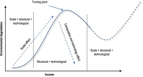
The EKC theory draws from two narratives: (i) interaction between scale, structure, and technology, and (ii) quality of life increases based on income increase (Ngarava et al. 2019). Increase in scale is associated with the increase in CO₂ emission. Structural changes also increase emissions, but to a lower extent and eventually lower it. Technology and R&D improves the efficiency and quality of environment. Other authors, such as Baek (2015), argue that instead of an inverted U-shape, the EKC is an inverted N-shape, with a last stage of increase in environmental degradation in a developed economy (Figure 1). In the quality-of-life proposition, more attention is given to better healthy consumption, environmental protection, and government intervention in environmental protection. The current study hypothesizes that economic diversification can lead to high CO₂ emissions, which is highly undesirable. However, high CO₂ emissions can also lead to economic diversification policies as mitigation strategy to curb unwarranted emissions. Thus, there is bi-directional dependence on each other. Various measures have been used in measuring diversification within an economy (Laverde-Rojas, Guevara-Fletcher, and Camacho-Murillo 2021). Product diversification was utilized by Mania (2020). Economic Complexity Index (ECI) was developed by Hidalgo and Hausmann (2009), enabling quantification of a country’s production through trade data interpretation. In this instance, a country’s income levels correlate with economic complexity. Authors, such as Neagu and Teodoru (2019), Doğan, Saboori, and Can (2019) as well as Can and Gozgor (2017), have utilized the ECI to ascertain whether product diversity has an impact on environmental degradation. There has been a divergence in the results obtained, offering an opportunity to ascertain how the interaction between environmental degradation and economic diversification plays out in a developing country such as South Africa.

Methodology

Economic diversification can be measured as the share of sectors in GDP, share of sectors in exports, dependence of a country on the export of a good, and the employment share of sectors. Measurement can be either from a country’s absolute specialization (e.g. diversification index, Gini index, Herfindahl-Hirshman index, entropy index, and ogive index) or from a country’s economic structure from a reference group of industries (e.g. inequality in productive sectors, relative Gini coefficient, and Theil index) (UNFCCC 2016a, 2016b). Tress Index (TI), as utilized by Meyer (2020), was used in the study. The current study is the first to utilize the TI in its association with CO₂ emissions. The TI indicates the level of concentration or diversification in a region’s economy (Quantec easydata 2021). It has a range of 0–100, where 0 represents a totally diversified economy, while a 100 represents a concentrated economy which is vulnerable to exogenous variables such as adverse climate change (Spocter 2012). A time series of the TI, which is increasing, reflects an expanding dependence of the local economy on a few or single economic activities, and increases vulnerability to climate change. The TI was ideal because it did not rely on exports, unlike the export diversification index. Furthermore, it considered the complexities within the economy relative to the Herfindahl-Hirshman index and concentrated on the contribution of each sector based on weighted averages relative to the entropy index which assumes an equi-proportional distribution (Bebczuk and Daniel Berrettoni 2006; Espoir 2020; Takada et al. 2020). There are 5 steps involved in calculating the TI (Quantec easydata 2021):

1. Calculating the contribution of each sector to the GDP;

2. Sector ranking based on contribution;

3. Multiplying each sector by its appropriate weighting;

4. Summing up the total weighted values of the sectors; and

5. Subtracting from the total and then dividing by the difference between the highest and lowest potential total weighted values.

The study utilized the TI of 10 industries, as prescribed by Quantec easydata (2021), which included (i) finance, insurance, real estate, and business services; (ii) manufacturing; (iii) general government; (iv) wholesale and retail trade, catering, and accommodation; (v) transport, storage, and communication; (vi) community, social, and personal services; (vii) agriculture, forestry, and fishing; (viii) construction; (ix) electricity, gas, and water; and (x) mining and quarrying. The TI index was calculated as follows: (1) $TI=\frac{\sum P_i{W}_i-W_l}{W_h-W_l}$(1) where $P_i$ is the percentage contribution of sector $i$ to the overall GDP, $W_i$ is the weight of sector $i$ based on ranked contribution to overall GDP (the higher the contribution, the higher the weight), $W_l$ is the lowest potential weight (which is 550 for 10 industries) and $W_h$ is the highest potential weight. The difference between the highest and lowest potential weights is 4.5 for 10 sectors (Quantec easydata 2021).

The study utilized the autoregressive distributed lag–error correction model (ARDL-ECM) to estimate the relationship between economic diversification and CO₂ emission, as well as other variables such as gross domestic product (GDP), population, foreign direct investment (FDI), and trade balance. This was modeled on the function shown in Equation (2). (2) $T{I}_t=f(\mathrm{C}{\mathrm{O}}_2\mathrm{e}\mathrm{m}\mathrm{i}\mathrm{s}\mathrm{s}\mathrm{i}\mathrm{o}{\mathrm{n}}_t\mathrm{G}\mathrm{r}\mathrm{o}\mathrm{s}\mathrm{s}\mathrm{D}\mathrm{o}\mathrm{m}\mathrm{e}\mathrm{s}\mathrm{t}\mathrm{i}\mathrm{c}\mathrm{P}\mathrm{r}\mathrm{o}\mathrm{d}\mathrm{u}\mathrm{c}{\mathrm{t}}_t\mathrm{P}\mathrm{o}\mathrm{p}\mathrm{u}\mathrm{l}\mathrm{a}\mathrm{t}\mathrm{i}\mathrm{o}{\mathrm{n}}_t\mathrm{F}\mathrm{o}\mathrm{r}\mathrm{e}\mathrm{i}\mathrm{g}\mathrm{n}\mathrm{D}\mathrm{i}\mathrm{r}\mathrm{e}\mathrm{c}\mathrm{t}\mathrm{I}\mathrm{n}\mathrm{v}\mathrm{e}\mathrm{s}\mathrm{t}\mathrm{m}\mathrm{e}\mathrm{n}{\mathrm{t}}_t\mathrm{T}\mathrm{r}\mathrm{a}\mathrm{d}\mathrm{e}\mathrm{b}\mathrm{a}\mathrm{l}\mathrm{a}\mathrm{n}\mathrm{b}\mathrm{c}{\mathrm{e}}_t)$(2) The ARDL-ECM was utilized by authors such as Can, Dogan, and Saboori (2020), Coulibaly and Akia (2017) as well as Laverde-Rojas, Guevara-Fletcher, and Camacho-Murillo (2021). According to Coulibaly and Akia (2017), ARDL distinguishes between endogenous and explanatory variables. Its model’s long-term estimates are super-coherent in small samples, providing unbiased coefficients and valid results even when explanatory variables are endogenous. It also has an advantage of application regardless of the order of the variables, either I(0) or I(1), and simultaneously estimates both long- and short-run parameters (Kohler 2013). The ARDL model was specified as follows (Adeleye 2018): (3) $Y_t={\alpha }_{0i}+{\sum }_{i=1}^p{\phi }_i{Y}_{t-i}+{\sum }_{i=0}^q{\text{β}}_i^{\mathrm{\prime }}{X}_{t-i}+{\mu }_{it}$(3) where $Y_i^{\mathrm{\prime }}$ was a vector and the variables in $(X_t^{\mathrm{\prime }}{)}^{\mathrm{\prime }}$ were allowed to be purely $I\left(0\right)$ or $I\left(1\right)$ or co-integrated; $\text{β}$ and $\phi$ were coefficients; $\alpha$ was the constant; $i=1,\dots ,k$; $p,q$ were optimal lag orders; ${\mu }_{it}$ was a vector of the error terms – unobservable zero mean white noise vector process. This was reduced to the following form: (4) $\mathrm{\Delta }\ln \mathrm{T}{\mathrm{I}}_t=a_{01}+b_{11}\ln \mathrm{T}{\mathrm{I}}_{t-1}+b_{21}\ln \mathrm{G}\mathrm{D}{\mathrm{P}}_{t-1}+b_{31}\ln \mathrm{C}{{\mathrm{O}}_2}_{t-1}+b_{41}\ln \mathrm{P}\mathrm{o}{\mathrm{p}}_{t-1}+b_{51}\ln \mathrm{F}\mathrm{D}{\mathrm{I}}_{t-1}+b_{61}\ln \mathrm{T}\mathrm{R}{\mathrm{D}}_{t-1}+\sum _{i=1}^p{a}_{1i}\mathrm{\Delta }\ln \mathrm{T}{\mathrm{I}}_{t-1}+\sum _{i=1}^q{a}_{2i}\mathrm{\Delta }\ln \mathrm{G}\mathrm{D}{\mathrm{P}}_{t-1}+\sum _{i=1}^q{a}_{3i}\mathrm{\Delta }\ln \mathrm{C}{{\mathrm{O}}_2}_{t-1}+\sum _{i=1}^q{a}_{4i}\mathrm{\Delta }\ln \mathrm{P}\mathrm{o}{\mathrm{p}}_{t-1}+\sum _{i=1}^q{a}_{5i}\mathrm{\Delta }\ln \mathrm{F}\mathrm{D}{\mathrm{I}}_{t-1}+\sum _{i=1}^q{a}_{6i}\mathrm{\Delta }\ln \mathrm{T}\mathrm{R}{\mathrm{D}}_{t-1}+{ϵ}_{1t}$(4)

(5) $\begin{array}{r}\mathrm{\Delta }\ln \mathrm{G}\mathrm{D}{\mathrm{P}}_t=a_{02}+b_{11}\ln \mathrm{T}{\mathrm{I}}_{t-1}+b_{22}\ln \mathrm{G}\mathrm{D}{\mathrm{P}}_{t-1}\\ +b_{32}\ln \mathrm{C}{{\mathrm{O}}_2}_{t-1}+b_{42}\ln \mathrm{P}\mathrm{o}{\mathrm{p}}_{t-1}+b_{52}\ln \mathrm{F}\mathrm{D}{\mathrm{I}}_{t-1}\\ +b_{62}\ln \mathrm{T}\mathrm{R}{\mathrm{D}}_{t-1}+\sum _{i=1}^p{a}_{1i}\mathrm{\Delta }\ln \mathrm{G}\mathrm{D}{\mathrm{P}}_{t-1}\\ +\sum _{i=1}^q{a}_{2i}\mathrm{\Delta }\ln \mathrm{T}{\mathrm{I}}_{t-1}+\sum _{i=1}^q{a}_{3i}\mathrm{\Delta }\ln \mathrm{C}{{\mathrm{O}}_2}_{t-1}\\ +\sum _{i=1}^q{a}_{4i}\mathrm{\Delta }\ln \mathrm{P}\mathrm{o}{\mathrm{p}}_{t-1}+\sum _{i=1}^q{a}_{5i}\mathrm{\Delta }\ln \mathrm{F}\mathrm{D}{\mathrm{I}}_{t-1}\\ +\sum _{i=1}^q{a}_{6i}\mathrm{\Delta }\ln \mathrm{T}\mathrm{R}{\mathrm{D}}_{t-1}+{ϵ}_{2t}\end{array}$(5)

(6) $\begin{array}{rl}\mathrm{\Delta }\ln \mathrm{C}{\mathrm{O}}_{2}t& =a_{03}+b_{11}\ln \mathrm{T}{\mathrm{I}}_{t-1}+b_{23}\ln \mathrm{G}\mathrm{D}{\mathrm{P}}_{t-1}\\ & +b_{33}\ln \mathrm{C}{\mathrm{O}}_{2\mathrm{t}-1}+b_{43}\ln \mathrm{P}\mathrm{o}{\mathrm{p}}_{t-1}\\ & -+b_{53}\ln \mathrm{F}\mathrm{D}{\mathrm{I}}_{t-1}+b_{63}\ln \mathrm{T}\mathrm{R}{\mathrm{D}}_{t-1}\\ & +\sum _{i=1}^p{a}_{1i}\mathrm{\Delta }\ln \mathrm{C}{{\mathrm{O}}_2}_{t-1}+\sum _{i=1}^q{a}_{2i}\mathrm{\Delta }\ln \mathrm{G}\mathrm{D}{\mathrm{P}}_{t-1}\\ & +\sum _{i=1}^q{a}_{3i}\mathrm{\Delta }\ln \mathrm{T}{\mathrm{I}}_{2\mathrm{t}-1}\end{array}$(6)

(7) $\begin{array}{rl}& \mathrm{\Delta }\ln \mathrm{P}\mathrm{o}{\mathrm{p}}_t=a_{04}+b_{11}\ln \mathrm{T}{\mathrm{I}}_{t-1}+b_{24}\ln \mathrm{G}\mathrm{D}{\mathrm{P}}_{t-1}\\ & +b_{34}\ln \mathrm{C}{{\mathrm{O}}_2}_{t-1}+b_{44}\ln \mathrm{P}\mathrm{o}{\mathrm{p}}_{t-1}+b_{54}\ln \mathrm{F}\mathrm{D}{\mathrm{I}}_{t-1}\\ & +b_{64}\ln \mathrm{T}\mathrm{R}{\mathrm{D}}_{t-1}+\sum _{i=1}^p{a}_{1i}\mathrm{\Delta }\ln \mathrm{P}\mathrm{o}{\mathrm{p}}_{t-1}\\ & +\sum _{i=1}^q{a}_{2i}\mathrm{\Delta }\ln \mathrm{G}\mathrm{D}{\mathrm{P}}_{t-1}+\sum _{i=1}^q{a}_{3i}\mathrm{\Delta }\ln \mathrm{C}{{\mathrm{O}}_2}_{t-1}\\ & +\sum _{i=1}^q{a}_{4i}\mathrm{\Delta }\ln \mathrm{T}{\mathrm{I}}_{t-1}+\sum _{i=1}^q{a}_{5i}\mathrm{\Delta }\ln \mathrm{F}\mathrm{D}{\mathrm{I}}_{t-1}\\ & +\sum _{i=1}^q{a}_{6i}\mathrm{\Delta }\ln \mathrm{T}\mathrm{R}{\mathrm{D}}_{t-1}+{ϵ}_{4t}\end{array}$(7) (8) $\begin{array}{rl}& \mathrm{\Delta }\ln \mathrm{F}\mathrm{D}{\mathrm{I}}_t=a_{05}+b_{11}\ln \mathrm{T}{\mathrm{I}}_{t-1}+b_{25}\ln \mathrm{G}\mathrm{D}{\mathrm{P}}_{t-1}\\ & +b_{35}\ln \mathrm{C}{{\mathrm{O}}_2}_{t-1}+b_{45}\ln \mathrm{P}\mathrm{o}{\mathrm{p}}_{t-1}+b_{55}\ln \mathrm{F}\mathrm{D}{\mathrm{I}}_{t-1}\\ & +b_{65}\ln \mathrm{T}\mathrm{R}{\mathrm{D}}_{t-1}+\sum _{i=1}^p{a}_{1i}\mathrm{\Delta }\ln \mathrm{F}\mathrm{D}{\mathrm{I}}_{t-1}\\ & +\sum _{i=1}^q{a}_{2i}\mathrm{\Delta }\ln \mathrm{G}\mathrm{D}{\mathrm{P}}_{t-1}+\sum _{i=1}^q{a}_{3i}\mathrm{\Delta }\ln \mathrm{C}{{\mathrm{O}}_2}_{t-1}\\ & +\sum _{i=1}^q{a}_{4i}\mathrm{\Delta }\ln \mathrm{P}\mathrm{o}{\mathrm{p}}_{t-1}+\sum _{i=1}^q{a}_{5i}\mathrm{\Delta }\ln \mathrm{T}{\mathrm{I}}_{t-1}\\ & +\sum _{i=1}^q{a}_{6i}\mathrm{\Delta }\ln \mathrm{T}\mathrm{R}{\mathrm{D}}_{t-1}+{ϵ}_{5t}\end{array}$(8)

(9) $\begin{array}{rl}& \mathrm{\Delta }\ln \mathrm{T}\mathrm{R}{\mathrm{D}}_t=a_{06}+b_{11}\ln \mathrm{T}{\mathrm{I}}_{t-1}+b_{26}\ln \mathrm{G}\mathrm{D}{\mathrm{P}}_{t-1}\\ & +b_{36}\ln \mathrm{C}{{\mathrm{O}}_2}_{t-1}+b_{46}\ln \mathrm{P}\mathrm{o}{\mathrm{p}}_{t-1}+b_{56}\ln \mathrm{F}\mathrm{D}{\mathrm{I}}_{t-1}\\ & +b_{66}\ln \mathrm{T}\mathrm{R}{\mathrm{D}}_{t-1}+\sum _{i=1}^p{a}_{1i}\mathrm{\Delta }\ln \mathrm{T}\mathrm{R}{\mathrm{D}}_{t-1}+\sum _{i=1}^q{a}_{2i}\mathrm{\Delta }\ln \\ & \mathrm{G}\mathrm{D}{\mathrm{P}}_{t-1}+\sum _{i=1}^q{a}_{3i}\mathrm{\Delta }\ln \mathrm{C}{{\mathrm{O}}_2}_{t-1}+\sum _{i=1}^q{a}_{4i}\mathrm{\Delta }\ln \mathrm{P}\mathrm{o}{\mathrm{p}}_{t-1}\\ & +\sum _{i=1}^q{a}_{5i}\mathrm{\Delta }\ln \mathrm{F}\mathrm{D}{\mathrm{I}}_{t-1}+\sum _{i=1}^q{a}_{6i}\mathrm{\Delta }\ln \mathrm{T}{\mathrm{I}}_{t-1}+{ϵ}_{6t}\end{array}$(9) where $\mathrm{T}\mathrm{I}$, $\mathrm{G}\mathrm{D}\mathrm{P}$, $\mathrm{C}{\mathrm{O}}_2$, $\mathrm{P}\mathrm{o}\mathrm{p}$, $\mathrm{F}\mathrm{D}\mathrm{I}$, $\mathrm{T}\mathrm{R}\mathrm{D}$_, and $ϵ$ are Tress Index, gross domestic product per capita, carbon dioxide emission (kilo-tons), population, foreign direct invest, trade balance, and error terms, respectively. All variables except the TI were at constant 2000 level. All variables were taken into logarithmic form before estimating the models. All the data were annual from 1993 to 2020, due to the fact that the TI recording in South Africa was started in 1993. The data were obtained from Quantec easydata (2021). These variables were included in the model due to the fact that they affect CO₂ emissions and economic diversification (Can, Dogan, and Saboori 2020). Tress Index (TI), FDI, and trade balance were expected to have a negative association with CO₂ emissions, while GDP and population were expected to have a positive association. Increase in TI indicates a concentrated economy which is less advanced and technologically friendly, therefore as diversification increases, CO₂ emission will decrease. Increase in FDI and trade balance will also improve the mix of activities in the economy and product diversity, respectively, thereby improving diversification and reducing CO₂ emission. Carbon dioxide (CO₂), GDP, FDI, population, and trade balance were expected to have a positive association with TI. Increase in TI indicates a more concentrated economy which is energy intensive. This is also the case of increase in GDP, while population increase induces pressure and demand on natural resources. A positive trade balance allows for specialization, reducing economic diversification.

The ARDL bounds model, which was used in the study, was based on the Wald statistic (F-statistic) for cointegration analysis (Odhiambo 2012). The null hypothesis of no cointegration was tested against the alternative of the existence of cointegration. If the F-statistic exceeded the critical bounds value, the H₀ was rejected, while it was not rejected when it is lower. If the statistic fell between the upper and lower bounds, then it was inconclusive. If no cointegration was detected, the following ARDL $p,q_1,q_2,q_3,q_4,q_5$ model was specified as follows:

(10) $\begin{array}{rl}& \mathrm{\Delta }\ln \mathrm{T}{\mathrm{I}}_t=a_{01}+\sum _{i=1}^p{a}_{1i}\mathrm{\Delta }\ln \mathrm{T}{\mathrm{I}}_{t-1}+\sum _{i=1}^q{a}_{2i}\mathrm{\Delta }\ln \mathrm{G}\mathrm{D}{\mathrm{P}}_{t-1}\\ & +\sum _{i=1}^q{a}_{3i}\mathrm{\Delta }\ln \mathrm{C}{{\mathrm{O}}_2}_{t-1}+\sum _{i=1}^q{a}_{4i}\mathrm{\Delta }\ln \mathrm{P}\mathrm{o}{\mathrm{p}}_{t-1}\\ & +\sum _{i=1}^q{a}_{5i}\mathrm{\Delta }\ln \mathrm{F}\mathrm{D}{\mathrm{I}}_{t-1}+\sum _{i=1}^q{a}_{6i}\mathrm{\Delta }\ln \mathrm{T}\mathrm{R}{\mathrm{D}}_{t-1}+{ϵ}_{1t}\end{array}$(10)

(11) $\begin{array}{rl}& \mathrm{\Delta }\ln \mathrm{G}\mathrm{D}{\mathrm{P}}_t=a_{02}+\sum _{i=1}^p{a}_{1i}\mathrm{\Delta }\ln \mathrm{G}\mathrm{D}{\mathrm{P}}_{t-1}+\sum _{i=1}^q{a}_{2i}\mathrm{\Delta }\ln \mathrm{T}{\mathrm{I}}_{t-1}\\ & +\sum _{i=1}^q{a}_{3i}\mathrm{\Delta }\ln \mathrm{C}{{\mathrm{O}}_2}_{t-1}+\sum _{i=1}^q{a}_{4i}\mathrm{\Delta }\ln \mathrm{P}\mathrm{o}{\mathrm{p}}_{t-1}\\ & +\sum _{i=1}^q{a}_{5i}\mathrm{\Delta }\ln \mathrm{F}\mathrm{D}{\mathrm{I}}_{t-1}+\sum _{i=1}^q{a}_{6i}\mathrm{\Delta }\ln \mathrm{T}\mathrm{R}{\mathrm{D}}_{t-1}+{ϵ}_{2t}\end{array}$(11)

(12) $\begin{array}{rl}& \mathrm{\Delta }\ln \mathrm{C}{\mathrm{O}}_{2}t=a_{03}+\sum _{i=1}^p{a}_{1i}\mathrm{\Delta }\ln \mathrm{C}{\mathrm{O}}_{2\mathrm{t}-1}\\ & +\sum _{i=1}^q{a}_{2i}\mathrm{\Delta }\ln \mathrm{G}\mathrm{D}{\mathrm{P}}_{t-1}+\sum _{i=1}^q{a}_{3i}\mathrm{\Delta }\ln \mathrm{T}{\mathrm{I}}_{2\mathrm{t}-1}\\ & +\sum _{i=1}^q{a}_{4i}\mathrm{\Delta }\ln \mathrm{P}\mathrm{o}{\mathrm{p}}_{t-1}+\sum _{i=1}^q{a}_{5i}\mathrm{\Delta }\ln \mathrm{F}\mathrm{D}{\mathrm{I}}_{t-1}\\ & +\sum _{i=1}^q{a}_{6i}\mathrm{\Delta }\ln \mathrm{T}\mathrm{R}{\mathrm{D}}_{t-1}+{ϵ}_{3t}\end{array}$(12)

(13) $\mathrm{\Delta }\ln \mathrm{P}\mathrm{o}{\mathrm{p}}_t=a_{04}+\sum _{i=1}^p{a}_{1i}\mathrm{\Delta }\ln \mathrm{P}\mathrm{o}{\mathrm{p}}_{t-1}+\sum _{i=1}^q{a}_{2i}\mathrm{\Delta }\ln \mathrm{G}\mathrm{D}{\mathrm{P}}_{t-1}+\sum _{i=1}^q{a}_{3i}\mathrm{\Delta }\ln \mathrm{C}{{\mathrm{O}}_2}_{t-1}+\sum _{i=1}^q{a}_{4i}\mathrm{\Delta }\ln \mathrm{T}{\mathrm{I}}_{t-1}+\sum _{i=1}^q{a}_{5i}\mathrm{\Delta }\ln \mathrm{F}\mathrm{D}{\mathrm{I}}_{t-1}+\sum _{i=1}^q{a}_{6i}\mathrm{\Delta }\ln \mathrm{T}\mathrm{R}{\mathrm{D}}_{t-1}+{ϵ}_{4t}$(13)

(14) $\mathrm{\Delta }\ln \mathrm{F}\mathrm{D}{\mathrm{I}}_t=a_{05}+\sum _{i=1}^p{a}_{1i}\mathrm{\Delta }\ln \mathrm{F}\mathrm{D}{\mathrm{I}}_{t-1}+\sum _{i=1}^q{a}_{2i}\mathrm{\Delta }\ln \mathrm{G}\mathrm{D}{\mathrm{P}}_{t-1}+\sum _{i=1}^q{a}_{3i}\mathrm{\Delta }\ln \mathrm{C}{{\mathrm{O}}_2}_{t-1}+\sum _{i=1}^q{a}_{4i}\mathrm{\Delta }\ln \mathrm{P}\mathrm{o}{\mathrm{p}}_{t-1}+\sum _{i=1}^q{a}_{5i}\mathrm{\Delta }\ln \mathrm{T}{\mathrm{I}}_{t-1}+\sum _{i=1}^q{a}_{6i}\mathrm{\Delta }\ln \mathrm{T}\mathrm{R}{\mathrm{D}}_{t-1}+{ϵ}_{5t}$(14)

(15) $\mathrm{\Delta }\ln \mathrm{T}\mathrm{R}{\mathrm{D}}_t=a_{06}+\sum _{i=1}^p{a}_{1i}\mathrm{\Delta }\ln \mathrm{T}\mathrm{R}{\mathrm{D}}_{t-1}+\sum _{i=1}^q{a}_{2i}\mathrm{\Delta }\ln \mathrm{G}\mathrm{D}{\mathrm{P}}_{t-1}+\sum _{i=1}^q{a}_{3i}\mathrm{\Delta }\ln \mathrm{C}{{\mathrm{O}}_2}_{t-1}+\sum _{i=1}^q{a}_{4i}\mathrm{\Delta }\ln \mathrm{P}\mathrm{o}{\mathrm{p}}_{t-1}+\sum _{i=1}^q{a}_{5i}\mathrm{\Delta }\ln \mathrm{F}\mathrm{D}{\mathrm{I}}_{t-1}+\sum _{i=1}^q{a}_{6i}\mathrm{\Delta }\ln \mathrm{T}{\mathrm{I}}_{t-1}+{ϵ}_{6t}$(15)

If cointegration was detected, the error correction model (ECM) was specified as follows:

(16) $\mathrm{\Delta }\ln \mathrm{T}{\mathrm{I}}_t=a_{01}+\sum _{i=1}^p{a}_{1i}\mathrm{\Delta }\ln \mathrm{E}{\mathrm{D}}_{t-1}+\sum _{i=1}^q{a}_{2i}\mathrm{\Delta }\ln \mathrm{G}\mathrm{D}{\mathrm{P}}_{t-1}+\sum _{i=1}^q{a}_{3i}\mathrm{\Delta }\ln \mathrm{C}{{\mathrm{O}}_2}_{t-1}+\sum _{i=1}^q{a}_{4i}\mathrm{\Delta }\ln \mathrm{P}\mathrm{o}{\mathrm{p}}_{t-1}+\sum _{i=1}^q{a}_{5i}\mathrm{\Delta }\ln \mathrm{F}\mathrm{D}{\mathrm{I}}_{t-1}+\sum _{i=1}^q{a}_{6i}\mathrm{\Delta }\ln \mathrm{T}\mathrm{R}{\mathrm{D}}_{t-1}+\lambda \mathrm{E}\mathrm{C}{\mathrm{T}}_{t-1}+{ϵ}_{1t}$(16)

(17) $\mathrm{\Delta }\ln \mathrm{G}\mathrm{D}{\mathrm{P}}_t=a_{02}+\sum _{i=1}^p{a}_{1i}\mathrm{\Delta }\ln \mathrm{G}\mathrm{D}{\mathrm{P}}_{t-1}+\sum _{i=1}^q{a}_{2i}\mathrm{\Delta }\ln \mathrm{T}{\mathrm{I}}_{t-1}+\sum _{i=1}^q{a}_{3i}\mathrm{\Delta }\ln \mathrm{C}{{\mathrm{O}}_2}_{t-1}+\sum _{i=1}^q{a}_{4i}\mathrm{\Delta }\ln \mathrm{P}\mathrm{o}{\mathrm{p}}_{t-1}+\sum _{i=1}^q{a}_{5i}\mathrm{\Delta }\ln \mathrm{F}\mathrm{D}{\mathrm{I}}_{t-1}+\sum _{i=1}^q{a}_{6i}\mathrm{\Delta }\ln \mathrm{T}\mathrm{R}{\mathrm{D}}_{t-1}+\lambda \mathrm{E}\mathrm{C}{\mathrm{T}}_{t-1}+{ϵ}_{2t}$(17)

(18) $\mathrm{\Delta }\ln \mathrm{C}{\mathrm{O}}_{2t}=a_{03}+\sum _{i=1}^p{a}_{1i}\mathrm{\Delta }\ln \mathrm{C}{{\mathrm{O}}_2}_{t-1}+\sum _{i=1}^q{a}_{2i}\mathrm{\Delta }\ln \mathrm{G}\mathrm{D}{\mathrm{P}}_{t-1}+\sum _{i=1}^q{a}_{3i}\mathrm{\Delta }\ln \mathrm{T}{{\mathrm{I}}_2}_{t-1}+\sum _{i=1}^q{a}_{4i}\mathrm{\Delta }\ln \mathrm{P}\mathrm{o}{\mathrm{p}}_{t-1}+\sum _{i=1}^q{a}_{5i}\mathrm{\Delta }\ln \mathrm{F}\mathrm{D}{\mathrm{I}}_{t-1}+\sum _{i=1}^q{a}_{6i}\mathrm{\Delta }\ln \mathrm{T}\mathrm{R}{\mathrm{D}}_{t-1}+\lambda \mathrm{E}\mathrm{C}{\mathrm{T}}_{t-1}+{ϵ}_{3t}$(18)

(19) $\mathrm{\Delta }\ln \mathrm{P}\mathrm{o}{\mathrm{p}}_t=a_{04}+\sum _{i=1}^p{a}_{1i}\mathrm{\Delta }\ln \mathrm{P}\mathrm{o}{\mathrm{p}}_{t-1}+\sum _{i=1}^q{a}_{2i}\mathrm{\Delta }\ln \mathrm{G}\mathrm{D}{\mathrm{P}}_{t-1}+\sum _{i=1}^q{a}_{3i}\mathrm{\Delta }\ln \mathrm{C}{{\mathrm{O}}_2}_{t-1}+\sum _{i=1}^q{a}_{4i}\mathrm{\Delta }\ln \mathrm{T}{\mathrm{I}}_{t-1}+\sum _{i=1}^q{a}_{5i}\mathrm{\Delta }\ln \mathrm{F}\mathrm{D}{\mathrm{I}}_{t-1}+\sum _{i=1}^q{a}_{6i}\mathrm{\Delta }\ln \mathrm{T}\mathrm{R}{\mathrm{D}}_{t-1}+\lambda \mathrm{E}\mathrm{C}{\mathrm{T}}_{t-1}+{ϵ}_{4t}$(19)

(20) $\mathrm{\Delta }\ln \mathrm{F}\mathrm{D}{\mathrm{I}}_t=a_{05}+\sum _{i=1}^p{a}_{1i}\mathrm{\Delta }\ln \mathrm{F}\mathrm{D}{\mathrm{I}}_{t-1}+\sum _{i=1}^q{a}_{2i}\mathrm{\Delta }\ln \mathrm{G}\mathrm{D}{\mathrm{P}}_{t-1}+\sum _{i=1}^q{a}_{3i}\mathrm{\Delta }\ln \mathrm{C}{{\mathrm{O}}_2}_{t-1}+\sum _{i=1}^q{a}_{4i}\mathrm{\Delta }\ln \mathrm{P}\mathrm{o}{\mathrm{p}}_{t-1}+\sum _{i=1}^q{a}_{5i}\mathrm{\Delta }\ln \mathrm{T}{\mathrm{I}}_{t-1}+\sum _{i=1}^q{a}_{6i}\mathrm{\Delta }\ln \mathrm{T}\mathrm{R}{\mathrm{D}}_{t-1}+\lambda \mathrm{E}\mathrm{C}{\mathrm{T}}_{t-1}+{ϵ}_{5t}$(20) (21) $\mathrm{\Delta }\ln \mathrm{T}\mathrm{R}{\mathrm{D}}_t=a_{06}+\sum _{i=1}^p{a}_{1i}\mathrm{\Delta }\ln \mathrm{T}\mathrm{R}{\mathrm{D}}_{t-1}+\sum _{i=1}^q{a}_{2i}\mathrm{\Delta }\ln \mathrm{G}\mathrm{D}{\mathrm{P}}_{t-1}+\sum _{i=1}^q{a}_{3i}\mathrm{\Delta }\ln \mathrm{C}{{\mathrm{O}}_2}_{t-1}+\sum _{i=1}^q{a}_{4i}\mathrm{\Delta }\ln \mathrm{P}\mathrm{o}{\mathrm{p}}_{t-1}+\sum _{i=1}^q{a}_{5i}\mathrm{\Delta }\ln \mathrm{F}\mathrm{D}{\mathrm{I}}_{t-1}+\sum _{i=1}^q{a}_{6i}\mathrm{\Delta }\ln \mathrm{T}{\mathrm{I}}_{t-1}+\lambda \mathrm{E}\mathrm{C}{\mathrm{T}}_{t-1}+{ϵ}_{6t}$(21) where $\mathrm{E}\mathrm{C}{\mathrm{T}}_{t-1}$ was the error correction term which should be negative and statistically significant. Post estimation techniques were employed after analyzing the short-run and long-run relationships. Diagnostic tests of normality, collinearity, heteroscedasticity, linearity, and stability were performed. The Jarque-Bera test was used to determine the distribution of the model. The Breush-Godfrey Serial Correlation test was used to examine the residuals for serial correlation and determine whether the residuals were independent. Heteroscedasticity was assessed for equality of variance spread through the Breusch–Pagan Godfrey test, while the Ramsey RESET Linearity test was used to ascertain linear relationships. The structural stability of the models was tested using the CUSUM of squares test.

Results

Descriptive statistics

Table 1 shows that for the period 1993–2020, there was a relatively more economic diversification in a Tress index of 10 industries relative to 50 industries. There was an average of 421 475.5 kilotons of CO₂ emissions, with US$3.45 billion FDI inflows. The country’s GDP alternated between US$115 and US$416 billion, while it was a net importer of US$10 thousand worth of goods and services.

Table 1. Descriptive statistics for the period 1993–2020.

Variable	Economic diversification (Tress index)		CO2 emission (kilotons)	FDI inflows (current US$) (million)	GDP (current US$) (billion)	Population (million)	Trade balance (current US$) (thousand)
	10 industries	50 industries
Mean	37.80	66.45	421,475.5	3 450	251	48.91	−10.79
Minimum	35.90	64.60	321,049.5	11.29	115	39.63	−30.18
Maximum	40.90	69.20	503,112.4	9 890	416	58.56	4.23
Std. Dev.	1.38	1.54	55,629.5	2 870	102	5.56	10.53
Skewness	0.60	0.51	−0.17	0.60	0.03	0.12	−0.32
Kurtosis	2.32	1.71	1.60	2.13	1.46	1.92	1.81
Jarque-Bera	2.18	3.05	2.06	2.46	2.67	1.37	2.04

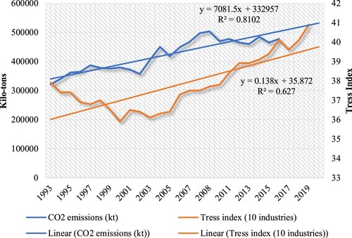
In the country, there was a gradual increase in the Tress Index and CO₂ emissions from 1993 to 2020 (Figure 2). The Tress Index increased by an average of 0.13 units annually, while the CO₂ emission increased by 7081 kilo-tons annually.

Figure 2. Tress index and CO₂ emission in South Africa (1993–2020).

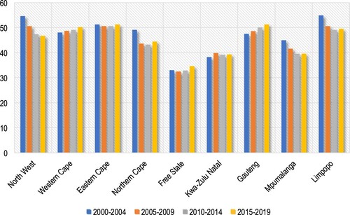
In South Africa, there has been a gradual economic concentration in Western Cape and Gauteng Provinces, as exhibited by the increase in the Tress indices (Figure 3). Provinces, such as North West, Mpumalanga and Limpopo, have been diversifying their economies since 2000.

Figure 3. Provincial tress indices (10 industries) between 2000 and 2020 in South Africa.

Empirical results

A unit root test was initially performed to test for stationarity and determine the order of integration. The unit root test in Table 2 shows that the variables were integrated at different orders, making the ARDL model ideal. Based on the Phillips-Perron (PP) Test, FDI, population and trade balance were stationery at levels, while economic diversity, CO₂ emissions, and GDP were stationery at first difference.

Table 2. Unit root test.

	Augmented Dickey Fuller (ADF) test		Philips-Perron (PP) test
	I (0)	I (1)	I (0)	I (1)
Tress index (TI)	0.99	−4.50***	1.18	−4.49***
CO2 emission index ($\mathrm{C}{\mathrm{O}}_2$)	−2.07	−4.97***	−2.12	−5.14***
FDI index ($\mathrm{F}\mathrm{D}\mathrm{I}$)	−4.70***	−109.30***	−145.78***	−109.30***
GDP index ($\mathrm{G}\mathrm{D}\mathrm{P}$)	−1.26	−3.77***	−1.09	−3.70**
Population index ($\mathrm{P}\mathrm{o}\mathrm{p}$)	−1.06	−1.85	−3.66**	−5.74***
Trade balance index ($\mathrm{T}\mathrm{R}\mathrm{D}$)	−2.09	−3.56**	−5.05***	−24.08***

***, **, and * indicate significance at 1%, 5%, and 10%, respectively.

Table 3 illustrates the lag selection criteria. This was performed to avoid bias and inefficiency when too few or too much lag lengths are selected. There were mixed lags from the different models based on the Akaike Information Criterion (AIC) and Schwarz Criterion (SC). A lag of 0 was obtained for CO₂ emissions and FDI models, while 1 was for GDP model and 4 for economic diversity, population, and trade balance models, respectively. The ARDL short-run and long-run were carried out using the AIC.

Table 3. Lag order selection criteria.

Lag	$\mathrm{T}\mathrm{I}$		$\mathrm{C}{\mathrm{O}}_2$		$\mathrm{F}\mathrm{D}\mathrm{I}$		$\mathrm{G}\mathrm{D}\mathrm{P}$		$\mathrm{P}\mathrm{o}\mathrm{p}$		$\mathrm{T}\mathrm{R}\mathrm{D}$
	AIC	SC	AIC	SC	AIC	SC	AIC	SC	AIC	SC	AIC	SC
0	2.20	2.50	5.61^a	5.67^a	11.14^a	11.44^a	7.68	7.98	5.25	5.55	18.50	18.80
1	1.10	1.45	5.66	5.73	11.15	11.50	7.35^a	7.70^a	−1.95	−1.61	18.59	18.94
2	1.20	1.60	5.76	5.83	11.24	11.64	7.45	7.84	−4.06	−3.66	18.62	19.02
3	0.95	1.40	5.83	5.92	11.20	11.65	7.43	7.88	−6.02	−5.57	18.35	18.80
4	0.72^a	1.22^a	5.92	6.02	11.18	11.68	7.53	8.02	−6.23^a	−5.73	18.17^a	18.67^a

^a Indicate Lag selection.

The ARDL Bounds test, indicated in Table 4, shows that there was a long-run equilibrium cointegration between the variables in all models, except the $\mathrm{G}\mathrm{D}\mathrm{P}$ model, which is inconclusive due to the fact that the F-statistic lies between the lower and upper bound at the 10% level. Thus, the ECM was necessary to specify the long-run models, except for the $\mathrm{G}\mathrm{D}\mathrm{P}$ model. Table 4 shows that in the short run, $\mathrm{G}\mathrm{D}\mathrm{P}$ had a positive relationship with $\mathrm{T}\mathrm{I}$, while $\mathrm{G}\mathrm{D}{\mathrm{P}}_{t-1}$, population, and $\mathrm{T}\mathrm{R}{\mathrm{D}}_{t-1}$ had a negative relationship with $\mathrm{T}\mathrm{I}$. In the short run, $\mathrm{C}{\mathrm{O}}_2$ emission had a positive relationship with $\mathrm{G}\mathrm{D}\mathrm{P}$ and $\mathrm{P}\mathrm{o}{\mathrm{p}}_{t-1}$, while it had a negative relationship with $\mathrm{P}\mathrm{o}\mathrm{p}$. In the short run, $\mathrm{T}{\mathrm{I}}_{t-1}$ had a negative relationship with $\mathrm{P}\mathrm{o}\mathrm{p}$ and a positive relationship with $\mathrm{T}\mathrm{R}\mathrm{D}$.

Table 4. ARDL Bounds Test.

Variable			$\mathrm{T}\mathrm{I}$		$\mathrm{C}{\mathrm{O}}_2$		$\mathrm{F}\mathrm{D}\mathrm{I}$		$\mathrm{G}\mathrm{D}\mathrm{P}$		$\mathrm{P}\mathrm{o}\mathrm{p}$		$\mathrm{T}\mathrm{R}\mathrm{D}$
$\mathrm{T}\mathrm{I}$					−2.66		42.65		16.96**		−0.11**		−691.28
${\mathrm{T}\mathrm{I}}_{t-1}$			0.32								−0.15***		3426.55*
$\mathrm{C}{\mathrm{O}}_2$			−0.02				1.00		1.49***		−0.007		54.28
$\mathrm{C}{{\mathrm{O}}_2}_{t-1}$			0.03		0.16		3.66		−0.78
$\mathrm{F}\mathrm{D}\mathrm{I}$			0.001		0.005				−0.03		0.0004		−4.01
$\mathrm{F}\mathrm{D}{\mathrm{I}}_{t-1}$			−5.98E-05				0.02**				−1.72E-05
$\mathrm{G}\mathrm{D}\mathrm{P}$			0.02**		0.28***		−1.22				0.004**		−18.88
$\mathrm{G}\mathrm{D}{\mathrm{P}}_{t-1}$			−0.02**						0.64**
$\mathrm{P}\mathrm{o}\mathrm{p}$			−1.77*		−15.31*		199.73		51.03**				10212.76
$\mathrm{P}\mathrm{o}{\mathrm{p}}_{t-1}$			1.64		14.74*		−189.24		−47.64**		0.95***		−9682.48
$\mathrm{T}\mathrm{R}\mathrm{D}$			−1.15E-05		8.15E-05		−0.002		4.13E-05		1.13E-05
$\mathrm{T}\mathrm{R}{\mathrm{D}}_{t-1}$			−6.95E-05**						0.001				−0.177
Constant			22.36673**		75.93		−1301.01		−553.09**		8.11***		−84913.86
Model summary
Adjusted R-squared			0.95		0.92		0.41		0.94		0.99		−0.12
Durbin-Watson statistic			1.82		1.95		3.00		2.28		1.55		2.06
F-statistic			41.76		37.51		2.94		36.73		58978.83		0.72
Prob (F-statistic)			0.000		0.000		0.037		0.000		0.000		0.68
Bounds test
	Sig.	I (0)	(1)
F-statistic	10%	2.26	3.35	4.44		5.61		2482.35		2.30		72.29		4.44
	5%	2.62	3.79
	2.5%	2.96	4.18
	1%	3.41	4.68

***, **, and * indicate significance at 1%, 5%, and 10%, respectively.

In the long run, $\mathrm{P}\mathrm{o}\mathrm{p}$ had a negative causal relationship with the $\mathrm{E}\mathrm{D}$, while $\mathrm{G}\mathrm{D}\mathrm{P}$ had a positive causal association with $\mathrm{C}{\mathrm{O}}_2$ emission (Table 5). $\mathrm{P}\mathrm{o}\mathrm{p}$ and $\mathrm{G}\mathrm{D}\mathrm{P}$ also had a positive association in the long run. A 1% increase in population increased economic diversity by 0.20%, whereas a 1% increase in economic concentration decreases the population by 4.74%. An increase of 1% in the GDP increased the CO₂ emissions by 0.33%. However, a 1% increase in CO₂ emissions increases GDP by 2.01%. Finally, a 1% increase in GDP increases population by 0.07%.

Table 5. Long-run relationship.

Variable	$\mathrm{T}\mathrm{I}$	$\mathrm{C}{\mathrm{O}}_2$	$\mathrm{F}\mathrm{D}\mathrm{I}$	$\mathrm{G}\mathrm{D}\mathrm{P}$	$\mathrm{P}\mathrm{o}\mathrm{p}$	$\mathrm{T}\mathrm{R}\mathrm{D}$
$\mathrm{T}\mathrm{I}$		−3.19	42.47	47.56	−4.74***	2323.11
$\mathrm{C}{\mathrm{O}}_2$	0.02		4.74	2.01*	−0.14	46.10
$\mathrm{F}\mathrm{D}\mathrm{I}$	0.002	0.006		−0.07	0.006	−3.41
$\mathrm{G}\mathrm{D}\mathrm{P}$	−0.003	0.33***	−1.24		0.07**	−16.04
$\mathrm{P}\mathrm{o}\mathrm{p}$	−0.20***	−0.68	10.68	9.53		450.37
$\mathrm{T}\mathrm{R}\mathrm{D}$	−0.0001	9.75E-05	−0.002	0.004	0.0002

***, **, and * indicate significance at 1%, 5%, and 10%, respectively.

The error correction terms indicate that there were long-run causal relationships in the models. In the economic diversity model, the reversion to long-run equilibrium was at an adjustment speed of 68%, and it will take 1.47 years (${\displaystyle \frac{1}{68\text{\%}}}$) to achieve this equilibrium. The speed of adjustment was at 84%, 98%, 36%, 5%, and 117% in the CO₂ emission, FDI, GDP, population, and trade balance indices models, respectively (Table 6). Time to restore equilibrium in the CO₂ emission model was 1.19 years, while it will take 1.02, 3.78, 20, and 0.85 years in the FDI, GDP, population, and trade balance models, respectively.

Table 6. Error correction model regression.

	$\mathrm{\partial }\mathrm{T}\mathrm{I}$	$\mathrm{\partial }\mathrm{C}{\mathrm{O}}_2$	$\mathrm{\partial }\mathrm{F}\mathrm{D}\mathrm{I}$	$\mathrm{\partial }\mathrm{G}\mathrm{D}\mathrm{P}$	$\mathrm{\partial }\mathrm{P}\mathrm{o}\mathrm{p}$	$\mathrm{\partial }\mathrm{T}\mathrm{R}\mathrm{D}$
$\mathrm{\partial }\mathrm{T}\mathrm{I}$					−0.11***	−691.28
$\mathrm{\partial }\mathrm{C}{\mathrm{O}}_2$	−0.02		1.00	1.49***
$\mathrm{\partial }\mathrm{F}\mathrm{D}\mathrm{I}$	0.001***				0.0004***
$\mathrm{\partial }\mathrm{G}\mathrm{D}\mathrm{P}$	0.02***
$\mathrm{\partial }\mathrm{P}\mathrm{o}\mathrm{p}$	−1.77***	−15.31***	199.73***	51.09***		10212.76***
$\mathrm{\partial }\mathrm{T}\mathrm{R}\mathrm{D}$	−1.15E-05			4.1E-05
Constant	22.37***	75.93***	−1301.01***	−553.09***	8.11***	−84913.86***
CointEq(−1)	−0.68***	−0.84***	−0.98***	−0.36***	−0.05***	−1.17***
Time to restore equilibrium (years)	1.47	1.19	1.02	2.78	20	0.85
Model summary
Adjusted R-squared	0.73	0.68	0.99	0.66	0.98	0.60
Durbin-Watson statistic	1.82	1.95	3.00	2.28	1.55	2.06
F-statistic	11.29***	24.02***	11617.67***	11.65***	400.82***	12.16***

***, **, and * indicate significance at 1%, 5%, and 10%, respectively.

Table 7 shows that CO₂ emission Granger caused economic diversification and FDI, while economic diversification caused FDI and population. Population Granger caused economic diversification, while GDP also Granger caused economic diversification.

Table 7. Pairwise Granger causality test.

Null hypothesis	F-statistic
$\mathrm{C}{\mathrm{O}}_2$ emissions index does not Granger cause $\mathrm{T}\mathrm{I}$	9.00***
$\mathrm{T}\mathrm{I}$ does not Granger cause $\mathrm{C}{\mathrm{O}}_2$ emissions	0.10
$\mathrm{F}\mathrm{D}\mathrm{I}$ index does not Granger cause $\mathrm{T}\mathrm{I}$	2.50
$\mathrm{T}\mathrm{I}$ does not Granger cause $\mathrm{F}\mathrm{D}\mathrm{I}$ index	4.94**
$\mathrm{G}\mathrm{D}\mathrm{P}$ index does not Granger cause $\mathrm{T}\mathrm{I}$	12.42***
$\mathrm{T}\mathrm{I}$ does not Granger cause $\mathrm{G}\mathrm{D}\mathrm{P}$ index	0.09
$\mathrm{P}\mathrm{o}\mathrm{p}$ does not Granger cause $\mathrm{T}\mathrm{I}$	10.88***
$\mathrm{T}\mathrm{I}$ does not Granger cause $\mathrm{P}\mathrm{o}\mathrm{p}$	93.24***
$\mathrm{T}\mathrm{R}\mathrm{D}$ does not Granger cause $\mathrm{T}\mathrm{I}$	2.49
$\mathrm{T}\mathrm{I}$ does not Granger cause $\mathrm{T}\mathrm{R}\mathrm{D}$	0.35
$\mathrm{F}\mathrm{D}\mathrm{I}$ index does not Granger cause $\mathrm{C}{\mathrm{O}}_2$ emissions	0.01
$\mathrm{C}{\mathrm{O}}_2$ emissions index does not Granger cause $\mathrm{F}\mathrm{D}\mathrm{I}$ Index	7.72**
$\mathrm{G}\mathrm{D}\mathrm{P}$ index does not Granger cause $\mathrm{C}{\mathrm{O}}_2$ emissions	2.06
$\mathrm{C}{\mathrm{O}}_2$ emissions index does not Granger cause $\mathrm{G}\mathrm{D}\mathrm{P}$ Index	0.11
$\mathrm{P}\mathrm{o}\mathrm{p}$ does not Granger cause $\mathrm{C}{\mathrm{O}}_2$ emissions	2.20
$\mathrm{C}{\mathrm{O}}_2$ emissions index does not Granger cause $\mathrm{P}\mathrm{o}\mathrm{p}$	0.05
$\mathrm{T}\mathrm{R}\mathrm{D}$ does not Granger cause $\mathrm{C}{\mathrm{O}}_2$ emissions	0.24
$\mathrm{C}{\mathrm{O}}_2$ emissions index does not Granger cause $\mathrm{T}\mathrm{R}\mathrm{D}$	0.49

*** and ** indicate significance at 1% and 5%, respectively.

From the diagnostics tests in Table 8, the Jarque-Bera normality test showed that the error terms were normally distributed in all models except the trade balance model. Thus, the estimates had minimum variance property. The Breusch–Godfrey Serial Correlation LM Test showed that the error terms were independent in all models, except for the FDI model, and thus do not rely on the previous periods’ value. The Breusch–Pagan Godfrey test indicated that there was no heteroscedasticity, except for the FDI model, and thus there was no constant variance and they were homoscedastic. The models were well specified, as indicated by the Ramsey RESET Linearity Test, except for the GDP and trade balance models, indicating linear relationship. The CUSUM of squares test showed that all models were structurally stable, except for the trade balance model, and thus suitable for long-run decisions. Thus, the Tress, CO₂, and population indices models were normally distributed, homoscedastic, had no collinearity, well-specified, and stable. However, there was collinearity and heteroscedasticity in the FDI index model as well as no normality and instability in the trade balance index model. The GDP model was not well specified. The diagnostic tests verify that the models for Tress index and CO₂ were valid.

Table 8. Diagnostic tests.

Test	$\mathrm{T}\mathrm{I}$	$\mathrm{C}{\mathrm{O}}_2$ emissions	$\mathrm{F}\mathrm{D}\mathrm{I}$	$\mathrm{G}\mathrm{D}\mathrm{P}$	$\mathrm{P}\mathrm{o}\mathrm{p}$	$\mathrm{T}\mathrm{R}\mathrm{D}$
Normality test
Jarque-Bera	0.17	2.04	0.289	0.766	4.02	83.344
	(0.916)	(0.360)	(0.865)	(0.682)	(0.134)	(0.000)
Multi-collinearity test
Breusch-Godfrey	0.05	0.02	7.72	1.01	1.19	0.135
Serial Correlation LM Test	(0.825)	(0.898)	(0.016)	(0.334)	(0.295)	(0.719)
Heteroskedasticity test
Breusch-Pagan	1.54	1.64	2.64	1.08	0.42	0.932
Godfrey	(0.224)	(0.1997)	(0.054)	(0.436)	(0.890)	(0.521)
Linearity test
Ramsey RESET	0.14	0.66	1.21	3.24	0.92	5.31
Test (t-statistic)	(0.892)	(0.518)	(0.247)	(0.007)	(0.375)	(0.000)
Stability test
CUSUM of squares

Discussion

In both the short and long run, Tress index had negative causality with population index. This indicates that the economy becomes more diverse as the population increases in both the short and long run. Yakushnina (2019) explains this relationship through the need of social infrastructure as the population grows. The social infrastructure is mainly through social security, health care, education, housing, and communal services, among others. The productive infrastructure will also require to be expanded through the development of the economic basis and improvement of the standard of living. This tends to lead to a more diversified economy. The quality-of-life needs of a growing portion of the population, as well as the need to improve job opportunities, reinforce the need for a diversified economy (Yakushnina 2019). However, Hidalgo (2009) postulates that economic complexity is a result of the complexity of an economic structure of only a proportion of a population. Rightly so, a class/social structure within a population also tends to drive diversity in needs, which mirrors complexity within an economy. The social structure within South Africa changed significantly since the end of apartheid in 1994. There was an increase in the black middle class. According to Yameogo et al. (2014) improving conditions of the middle class of emerging economies was necessitated by the expansion of manufacturing sectors in countries that had relied on the extractive and agricultural (primary) industries. However, this expansion has increased structural transformation and economic diversity within such countries.

The study, however, found that economic diversity had no association with CO₂ emissions in the long run. This was in line with Laverde-Rojas, Guevara-Fletcher, and Camacho-Murillo (2021) findings in Colombia of the lack of benefit in increased economic complexity. This was contrary to Neagu and Teodoru (2019) who found economic complexity having an impact on greenhouse gas emissions, especially in countries with the lower level of economic complexity in the EU. This was observed in the short-run Granger causality test in the current study. The findings were also contrary to Dogan et al. (2021) as well as Doğan, Saboori, and Can (2019) who found economic complexity increasing environmental degradation in the lower and higher middle-income countries, while controlling CO₂ emissions in high-income countries. In France, Can and Gozgor (2017) identified that economic complexity suppresses CO₂ emissions in the long run. The major explanation can be in the differing measures of economic complexity and economic diversification. Economic complexity goes beyond economic diversification to include the quality and network positions in a knowledge economy (Ferraz et al. 2021). The result can also be due to the fact that South Africa has not reached the latter stages of development where technological advances and their associated diversification outweigh scale effects in growth. Thus, in the short run, CO₂ Granger caused economic diversity but in the long run, there was no association. In a study in Japan, Okamoto (2013) highlighted that structural change in an economy improves the environment. Gross Domestic Product (GDP) also caused economic diversity, while population had bi-directional causality with economic diversity, in the short run.

Carbon dioxide (CO₂) emissions index had a positive association with GDP index in both the short and long run. An increase in GDP increases CO₂ emission in both the short and long run. The findings were similar to Dogan et al. (2021), Simbi et al. (2021) as well as Menyah and Wolde-Rufael (2010) who highlighted that GDP was positively associated with CO₂ emissions. This is due to the fact that economic progress and development incite CO₂ emission increase through the scale effect of growth trajectory (Joshua, Bekun, and Sarkodie 2020). This is due to the dependence on highly emitting energy sources (Dogan et al. 2021). In South Africa, it is difficult to reduce CO₂ emissions without compromising economic growth (Menyah and Wolde-Rufael 2010). Waheed, Sarwar, and Wei (2019) highlight that this was mainly evident in developing countries and not evident in developed countries. However, Bekun, Emir, and Sarkodie (2019) found that in South Africa, an increase in economic activities decreased CO₂ emissions. Acheampong (2018) actually found out that it is CO₂ emissions which cause economic growth rather than the other way around.

Population index had positive causality with GDP in both the short and long run. In the short and long run, a rise in population increased GDP. Dogan et al. (2021) attributes this to an increase in several human activities within an economy as the population increases. However, Peterson (2017) attests that economic growth in high-income countries will be stifled by low population growth, while high population growth in low-income countries will slow down development. Joshua, Bekun, and Sarkodie (2020) denotes that population increase is associated with population explosion with urbanization increasing commercial activities. However, Omri, Nguyen, and Rault (2014) found to the contrary, indicating that population had a negative effect on CO₂ emissions.

Conclusion

The objective of the study was to ascertain the relationship between economic diversification and CO₂ emission in South Africa. The study found that in the short run, CO₂ Granger caused economic diversity but in the long run, there was no association. The study fails to reject the hypothesis of no bi-directional relationship between economic diversification and CO₂ emission, and concludes of a unidirectional causality in the short run and no relationship in the long run. The study suggests that South Africa is still in the latter stage of the scale phase of the EKC model, due to economic diversification (with its associated growth) having indifference relationship with CO₂ emissions. On one hand, the long- and short-run relationship between economic diversification and population augment this conclusion based on the social and productive infrastructural transformation pushing this relationship. Furthermore, the short-run relationship suggests that the country is still in the scale phase where expansion and growth (with its associated diversification) drive CO₂ emissions. Policy implications include the consideration of economic diversity in national, economic, and climate change policies such as the National Development Plan (NDP), National Industrial Policy Framework (NIPF), and National Determined Contributions (NDC). A balance needs to be struck between the scale effects of economic growth and structural, as well as technological, effects incorporating social and productive transformation and the associated economic diversification. This will overall have a reductive effect on CO₂ emissions. Economic diversification should be considered as an environmental pollution policy tool in the short run. This can be through active promotion of environment-friendly economic transformation, for example, utilization of renewable products and services, which will meet the country’s NDP, NIPF, and NDCs. The conclusion that the country is in the latter phase of the scale phase in the EKC theory indicates that the country will still be energy reliant in the short term. Policy should be focused on transitioning to renewable energy to improve growth while improving environmental sustainability. Furthermore, the EKC theory should be further expanded to include the effects of economic diversification and complexity to improve its utilization in policy.

Disclosure statement

No potential conflict of interest was reported by the author(s).

References

- Acheampong, Alex O. 2018. “Economic Growth, CO2 Emissions and Energy Consumption: What Causes What and Where?” Energy Economics 74: 677–692. doi:https://doi.org/10.1016/j.eneco.2018.07.022.
- Adebayo, Tomiwa Sunday, and Jamiu Adetola Odugbesan. 2021. “Modeling CO2 Emissions in South Africa: Empirical Evidence from ARDL Based Bounds and Wavelet Coherence Techniques.” Environmental Science and Pollution Research 28 (8): 9377–9389. doi:https://doi.org/10.1007/s11356-020-11442-3.
- Adeleye, Ngozi. 2018. “Autoregressive Distributed Lag (ARDL): Specification.” http://cruncheconometrix.org.ng.
- Baek, Jungho. 2015. “Environmental Kuznets Curve for CO2 Emissions: The Case of Arctic Countries.” Energy Economics 50: 13–17. doi:https://doi.org/10.1016/j.eneco.2015.04.010.
- Bebczuk, Ricardo N., and N. Daniel Berrettoni. 2006. “Explaining Export Diversification: An Empirical Analysis.” Caf Research Program on Development Issues. Argentina. https://www.caf.com/media/29872/rricardobebczuk-explainingexportsdiversification.pdf.
- Beidari, Mohamed, Sue Jane Lin, and Charles Lewis. 2017. “Decomposition Analysis of CO2 Emissions from Coal-Sourced Electricity Production in South Africa.” Aerosol and Air Quality Research 17 (4): 1043–1051. doi:https://doi.org/10.4209/aaqr.2016.11.0477.
- Bekhet, Hussain Ali, Ali Matar, and Tahira Yasmin. 2017. “CO2 Emissions, Energy Consumption, Economic Growth, and Financial Development in GCC Countries: Dynamic Simultaneous Equation Models.” Renewable and Sustainable Energy Reviews 70: 117–132. doi:https://doi.org/10.1016/j.rser.2016.11.089.
- Bekun, Festus Victor, Fırat Emir, and Samuel Asumadu Sarkodie. 2019. “Another Look at the Relationship Between Energy Consumption, Carbon Dioxide Emissions, and Economic Growth in South Africa.” Science of the Total Environment 655: 759–765. doi:https://doi.org/10.1016/j.scitotenv.2018.11.271.
- Bento, Cerdeira, João Paulo, and Victor Moutinho. 2016. “CO2 Emissions, Non-Renewable and Renewable Electricity Production, Economic Growth, and International Trade in Italy.” Renewable and Sustainable Energy Reviews 55: 142–155. doi:https://doi.org/10.1016/j.rser.2015.10.151.
- Bélaïd, Fateh, and Meriem Youssef. 2017. “Environmental Degradation, Renewable and Non-Renewable Electricity Consumption, and Economic Growth: Assessing the Evidence from Algeria.” Energy Policy 102: 277–187. doi:https://doi.org/10.1016/j.enpol.2016.12.012.
- Can, Muhlis, Munir Ahmad, and Zeeshan Khan. 2021. “The Impact of Export Composition on Environment and Energy Demand: Evidence from Newly Industrialized Countries.” Environmental Science and Pollution Research 28 (25): 33599–33612. doi:https://doi.org/10.1007/s11356-021-13084-5.
- Can, Muhlis, Buhari Dogan, and Behnaz Saboori. 2020. “Does Trade Matter for Environmental Degradation in Developing Countries? New Evidence in the Context of Export Product Diversification.” Environmental Science and Pollution Research 27 (13): 14702–14710. doi:https://doi.org/10.1007/s11356-020-08000-2.
- Can, Muhlis, and Giray Gozgor. 2017. “The Impact of Economic Complexity on Carbon Emissions: Evidence from France.” Environmental Science and Pollution Research 24 (19): 16364–16370. doi:https://doi.org/10.1007/s11356-017-9219-7.
- Coulibaly, Gninlgonakan Romaric, and Sosthène Alban Akia. 2017. “Export Structure and Economic Growth in a Developing Country: Case of Cote d’Ivoire.” Munich Personal RePEc Archive, no. 94116. https://mpra.ub.uni-muenchen.de/id/eprint/91374.
- Doğan, Buhari, Behnaz Saboori, and Muhlis Can. 2019. “Does Economic Complexity Matter for Environmental Degradation? An Empirical Analysis for Different Stages of Development.” Environmental Science and Pollution Research 26 (31): 31900–31912. doi:https://doi.org/10.1007/s11356-019-06333-1.
- Dogan, Buhari, Oana M Driha, Daniel B Lorente, and Umer Shahzad. 2021. “The Mitigating Effects of Economic Complexity and Renewable Energy on Carbon Emissions in Developed Countries.” Sustainable Development 29: 1–12. doi:https://doi.org/10.1002/sd.2125.
- DoTIC. 2021. “Why South Africa?” Pretoria. http://www.investsa.gov.za/.
- Espoir, Lukau Matezo. 2020. “Determinant of Export Diversification: An Empirical Analysis in the Case of SADC Countries.” International Journal of Research In Business and Social Science 9 (7): 130–144. doi:https://doi.org/10.20525/ijrbs.v9i7.942.
- Ferraz, Diogo, Fernanda P.S. Falguera, Enzo B. Mariano, and Dominik Hartmann. 2021. “Linking Economic Complexity, Diversification, and Industrial Policy with Sustainable Development: A Structured Literature Review.” Sustainability 13 (3): 1–29. doi:https://doi.org/10.3390/su13031265.
- Guo, Jiajia, Yong Zhou, Shahid Ali, Umer Shahzad, and Lianbiao Cui. 2021. “Exploring the Role of Green Innovation and Investment in Energy for Environmental Quality: An Empirical Appraisal from Provincial Data of China.” Journal of Environmental Management 292 (February): 112779. doi:https://doi.org/10.1016/j.jenvman.2021.112779.
- Hausmann, Ricardo, César A. Hidalgo, Sebastian Bustos, Michele Coscia, Sarah Chung, Juan Jimenez, Alexander Simoes, and Muhammed A. Yildirim. 2013. “Atlas of Economic Complexity.” In Atlas of Econ. Complexity, edited by Ricardo Hausmann, and César A Hidalgo. Massachusetts: MIT Press. https://atlas.cid.harvard.edu/countries/179%0Ahttps://atlas.cid.harvard.edu/glossary.
- Hidalgo, César A. 2009. “The Dynamics of Economic Complexity and the Product Space Over a 42 Year Period.” CID Working Paper Series 2009. Cambridge. doi:https://doi.org/10.1080/10835547.2012.12090314.
- Hidalgo, César A., and Ricardo Hausmann. 2009. “The Building Blocks of Economic Complexity.” Proceedings of the National Academy of Sciences of the United States of America 106 (26): 10570–10575. doi:https://doi.org/10.1073/pnas.0900943106.
- Ikram, Majid, Wanjun Xia, Zeeshan Fareed, Umer Shahzad, and Muhammad Zahid Rafique. 2021. “Exploring the Nexus Between Economic Complexity, Economic Growth and Ecological Footprint: Contextual Evidences from Japan.” Sustainable Energy Technologies and Assessments 47 (May): 101460. doi:https://doi.org/10.1016/j.seta.2021.101460.
- Inoua, Sabiou M. 2021. “A Simple Measure of Complexity.” ESI Working Paper, 21–11. https://digitalcommons.chapman.edu/ esi_working_papers/348.
- Joshua, Udi, Festus Victor Bekun, and Samuel Asumadu Sarkodie. 2020. “New Insight into the Causal Linkage Between Economic Expansion, FDI, Coal Consumption, Pollutant Emissions and Urbanization in South Africa.” Environmental Science and Pollution Research 27 (15): 18013–18024. doi:https://doi.org/10.1007/s11356-020-08145-0.
- Jury, Mark R. 2002. “Economic Impacts of Climate Variability in South Africa and Development of Resource Prediction Models.” Journal of Applied Meteorology 41 (1): 46–55. doi:https://doi.org/10.1175/1520-0450(2002)041<0046:EIOCVI>2.0.CO;2.
- Kohler, Marcel. 2013. “CO2 Emissions, Energy Consumption, Income and Foreign Trade: A South African Perspective.” Energy Policy 63: 1042–1050. doi:https://doi.org/10.1016/j.enpol.2013.09.022.
- Kwakwa, Paul Adjei, and Frank Adusah-Poku. 2020. “The Carbon Dioxide Emission Effects of Domestic Credit and Manufacturing Indicators in South Africa.” Management of Environmental Quality: An International Journal 31 (6): 1531–1548. doi:https://doi.org/10.1108/MEQ-11-2019-0245.
- Laverde-Rojas, Henry, Diego A. Guevara-Fletcher, and Andrés Camacho-Murillo. 2021. “Economic Growth, Economic Complexity, and Carbon Dioxide Emissions: The Case of Colombia.” Heliyon 7 (6): e07188. doi:https://doi.org/10.1016/j.heliyon.2021.e07188.
- Mania, Elodie. 2020. “Export Diversification and CO2 Emissions: An Augmented Environmental Kuznets Curves.” Journal of International Development 32: 168–185. doi:https://doi.org/10.1002/jid.
- Menyah, Kojo, and Yemane Wolde-Rufael. 2010. “Energy Consumption, Pollutant Emissions and Economic Growth in South Africa.” Energy Economics 32 (6): 1374–1382. doi:https://doi.org/10.1016/j.eneco.2010.08.002.
- Meyer, Daniel Francois. 2020. “Does the Diversification of the Economy Matter ? An Assessment of the Situation in South Africa.” EuroEconomica 2 (39): 181–194.
- Mirza, Faisal Mehmood, and Afra Kanwal. 2017. “Energy Consumption, Carbon Emissions and Economic Growth in Pakistan: Dynamic Causality Analysis.” Renewable and Sustainable Energy Reviews 72: 1233–1240. doi:https://doi.org/10.1016/j.rser.2016.10.081.
- Moutinho, Victor, Mara Madaleno, and Mohamed Elheddad. 2020. “Determinants of the Environmental Kuznets Curve Considering Economic Activity Sector Diversification in the OPEC Countries.” Journal of Cleaner Production 271: 122642. doi:https://doi.org/10.1016/j.jclepro.2020.122642.
- Neagu, Olimpia, and Mircea Constantin Teodoru. 2019. “The Relationship Between Economic Complexity, Energy Consumption Structure and Greenhouse Gas Emission: Heterogeneous Panel Evidence from the EU Countries.” Sustainability 11: 2. doi:https://doi.org/10.3390/su11020497.
- Ngarava, Saul, Leocadia Zhou, James Ayuk, and Simbarashe Tatsvarei. 2019. “Achieving Food Security in a Climate Change Environment: Considerations for Environmental Kuznets Curve Use in the South African Agricultural Sector.” Climate 7 (9): 108. doi:https://doi.org/10.3390/cli7090108.
- Odhiambo, Nicholas M. 2012. “Economic Growth and Carbon Emissions in South Africa: An Empirical Investigation.” The Journal of Applied Business Research 28 (1): 75–84.
- Okamoto, S. 2013. “Impacts of Growth of a Service Economy on CO2 Emissions: Japan’s Case.” Journal of Economic Structure 2: 8. doi:https://doi.org/10.1186/2193-2409-2-8.
- Omri, Anis, Duc Khuong Nguyen, and Christophe Rault. 2014. “Causal Interactions Between CO2 Emissions, FDI, and Economic Growth: Evidence from Dynamic Simultaneous-Equation Models.” Economic Modelling 42: 382–389. doi:https://doi.org/10.1016/j.econmod.2014.07.026.
- Peterson, Wesley E F. 2017. “The Role of Population in Economic Growth.” SAGE Open 7: 4. doi:https://doi.org/10.1177/2158244017736094.
- Plooy, Peet du, and Meagan Jooste. 2011. “Tade and Climate Change: Policy and Economic Implications for South Africa.” Pretoria.
- Proctor, Felicity J. 2014. “Rural Economic Diversification in Sub-Saharan Africa.” IIED Working Paper. London. http://pubs.iied.org/14632IIED.
- Quantec easydata. 2021. “Tress Index for GVA at Basic Prices.” Pretoria.
- Sarwar, Suleman, Umer Shahzad, Dongfeng Chang, and Biyan Tang. 2019. “Economic and Non-Economic Sector Reforms in Carbon Mitigation: Empirical Evidence from Chinese Provinces.” Structural Change and Economic Dynamics 49 (February): 146–154. doi:https://doi.org/10.1016/j.strueco.2019.01.003.
- Shahzad, Umer, Diogo Ferraz, Buhari Doğan, and Daisy Aparecida do Nascimento Rebelatto. 2020. “Export Product Diversification and CO2 Emissions: Contextual Evidences from Developing and Developed Economies.” Journal of Cleaner Production 276, doi:https://doi.org/10.1016/j.jclepro.2020.124146.
- Shikwambana, Lerato, Paidamwoyo Mhangara, and Mahlatse Kganyago. 2021. “Assessing the Relationship Between Economic Growth and Emissions Levels in South Africa Between 1994 and 2019.” Sustainability (Switzerland) 13 (5): 1–15. doi:https://doi.org/10.3390/su13052645.
- Simbi, Habiman Claudien, Jianyi Lin, Dewei Yang, Jean Claude Ndayishimiye, Yang Liu, Huimei Li, Lingxing Xu, and Weijing Ma. 2021. “Decomposition and Decoupling Analysis of Carbon Dioxide Emissions in African Countries During 1984–2014.” Journal of Environmental Sciences (China) 102: 85–98. doi:https://doi.org/10.1016/j.jes.2020.09.006.
- Spocter, Manfred. 2012. Using Geospatial Data Analysis and Qualitative Economic Intelligence to Inform Local Economic Development in Small Towns: A Case Study of Graaff-Reinet, South Africa. Johannesburg: Nova Science Publishers.
- Strambo, Claudia, and Aaron Atteridge. 2021. Collapse of the Free State Goldfields, South Africa: Lessons for Industrial Transitions. Stockholm: Stockholm Environmental Institute.
- Strambo, Claudia, Jesse Burton, and Aaron Atteridge. 2019. The End of Coal? Planning a ‘Just Transition’ in South Africa. Stockholm. https://cdn.sei.org/wp-content/uploads/2019/02/planning-a-just-transition-in-south-africa.pdf.
- Takada, Hellinton H., Celma O. Ribeiro, Oswaldo L.V. Costa, and Julio M. Stern. 2020. “Gini and Entropy-Based Spread Indexes for Primary Energy Consumption Efficiency and CO2 Emission.” Energies 13 (18): 1–17. doi:https://doi.org/10.3390/en13184938.
- TIPS. 2016. Analysis of Existing Industrial Policies and the State of Implementation in South Africa. Pretoria. www.tips.org.za.
- Trollip, Hilton, and Michael Boulle. 2017. “Challenges Associated with Implementing Climate Change Mitigation Policy in South Africa.” Cape.
- UNFCCC. 2009. “Report on the Technical Workshop on Increasing Economic Resilience to Climate Change and Reducing Reliance on Vulnerable Economic Sectors, Including through Economic Diversification.” Copenhagen.
- UNFCCC. 2016a. “The Concept of Economic Diversification in the Context of Response Measures.” Technical Paper, no. FCCC/TP/2016/3.
- UNFCCC. 2016b. The Concept of Economic Diversification in the Context of Response Measures Technical Paper by the Secretariat. Vol. TP/2016/3. Geneva: United Nations Framework Convention on Climate Change (UNFCCC).
- Waheed, Rida, S. Sarwar, and Chen Wei. 2019. “The Survey of Economic Growth, Energy Consumption and Carbon Emission.” Energy Reports 5: 1103–1115. doi:https://doi.org/10.1016/j.egyr.2019.07.006.
- Wang, Kai Hua, Muhammad Umar, Rabia Akram, and Ersin Caglar. 2021. “Is Technological Innovation Making World ‘Greener’? An Evidence from Changing Growth Story of China.” Technological Forecasting and Social Change 165: 120516. doi:https://doi.org/10.1016/j.techfore.2020.120516.
- Wewege, Sarah Jo. 2013. Economic Complexity and the Potential for Green Growth in South Africa. Cape Town: University of Cape Town.
- Winkler, Harald, and Andrew Marquand. 2009. “Changing Development Paths: From an Energy-Intensive to Low-Carbon Economy in South Africa.” Climate and Development 1 (1): 47–65. doi:https://doi.org/10.3763/cdev.2009.0003.
- Yakushnina, Tatyana. 2019. “Some Features of Rural Economic Diversification in Mining Regions.” E3S Web of Conferences 134: 10–14. doi:https://doi.org/10.1051/e3sconf/201913403018.
- Yameogo, Nadege Desiree, Tiguene Nabassaga, Abebe Shimeles, and Mthuli Ncube. 2014. “Diversification and Sophistication as Drivers of Structural Transformation for Africa: The Economic Complexity Index of African Countries.” Journal of African Development 16 (2): 1–31.