Characterising driver heterogeneity within stochastic traffic simulation

ABSTRACT

Drivers’ heterogeneity and the broad range of vehicle characteristics on public roads are primarily responsible for the stochasticity observed in road traffic dynamics. Understanding the behavioural differences in drivers (human or automated systems) and reproducing observed behaviours in microsimulation has lately attracted significant attention. Calibration of car-following model parameters is the prevalent way to chracterize different driving behaviours. However, most car-following models do not realistically reproduce free-flow accelerations and therefore, model parameters are usually mainly the result of over-fitting with limited possibility to reproduce realistic drivers’ heterogeneity in simulation. To solve this problem, the present study proposes a novel framework to identify individual driver fingerprints based on their acceleration behaviours and reproduce them in microsimulation. The paper also discusses the unsuitability of vehicle acceleration to properly characterise alone the aggressiveness of a driver. A large experimental campaign and simulation results demonstrate the robustness of the proposed method.

KEYWORDS:

• Drivers’ heterogeneity
• driving behaviour
• stochastic traffic simulation
• vehicles’ dynamics
• microscopic free-flow acceleration model (MFC)

1. Introduction

Variability in the behaviour of human drivers and vehicle dynamics are responsible for the emergence of stochastic patterns in the way vehicles move and interact. Traffic flow is composed of many heterogeneous vehicles in terms of power dynamics, powertrains and vehicle manufacturers, which are driven by heterogeneous drivers. On a macroscopic scale, this heterogeneity has been linked to the evolution of several traffic-related phenomena such as capacity drop, traffic hysteresis, traffic oscillations, and stop and go waves, to name a few (Chen et al. 2014; Huang et al. 2018; Laval and Leclercq 2010; Saifuzzaman et al. 2017; Zheng et al. 2011). Consequently, properly characterising this heterogeneity and reproducing it within microsimulation has attracted significant interest in the literature. However, the attention has been mainly focused on the heterogeneity of the drivers’ style and significantly less attention has been paid to understand the impact of the heterogeneity in the vehicles.

Several attempts to characterise driver heterogeneity have been carried out in the past decades. In general, research efforts have so far focused on the variability in the behaviour of the same driver, called intra-driver heterogeneity (Berthaume et al. 2018; Huang et al. 2018; Wang et al. 2010), or of different drivers, called inter-driver heterogeneity (Taylor et al. 2015), or both (Ossen and Hoogendoorn 2011). Heterogeneity has been linked to several factors such as the driver's personal information (gender, age, etc.) (Yagil 1998; Nagahama, Yanagisawa, and Nishinari 2020) weather conditions (Kilpeläinen and Summala 2007), traffic conditions (Lajunen, Parker, and Summala 1999), mood (Underwood et al. 1999) and cross-cultural differences (Özkan et al. 2006) and in some cases it is handled through fuzzy interpretations (Aghabayk, Forouzideh, and Young 2013a), considering also the task difficulty (Li, Li, and Ni 2021). Traffic conditions could induce variability also for systems of low driving automation levels (Alhariqi, Gu, and Saberi 2022). The effect of the vehicle type, or powertrain has been shown to directly affect the acceleration behaviour (Nagahama, Yanagisawa, and Nishinari 2020). Heterogeneity has been recognised, not only in the longitudinal control, but also in the lateral control, between different drivers, and different vehicles (Li et al. 2022; Raju et al. 2022). Several attempts have been made to cluster similar driving traits. This has usually involved naturalistic driving data collection from experiments and/or information extraction using statistical learning methods (Al Haddad and Antoniou 2022).

With the advent of automated driver assistance systems, such as Adaptive Cruise Control (ACC), a reduction (at least) in drivers’ heterogeneity and most probably also in the variety of the observed vehicle dynamics is expected (Makridis et al. 2021). This gives an additional motivation to gain a deeper understanding and accurate description of observed driving behaviour, as this would facilitate meaningful comparative studies between human and automated drivers (Calvert and van Arem 2020; Zhao et al. 2020). Moreover, solutions of vehicle connectivity that are being developed could amplify both inter-driver and intra-driver behaviour variations (T. Li et al. 2020).

Within microscopic traffic models, car-following models reproduce the longitudinal driving task. Different driver behaviours are captured stochastically, injecting white noise on the model’s acceleration parameter (Laval, Toth, and Zhou 2014; Ngoduy et al. 2019; Treiber, Kesting, and Helbing 2006; Treiber and Kesting 2013). Stochasticity in the acceleration behaviour has been identified as one of the main sources of capacity drop (Yuan et al. 2019). Among several other factors, such implementations aim to reproduce the intrinsic stochasticity, observed in human drivers (Jiang et al. 2015). We argue that there is room for improvement concerning the explicit reproduction in the variability of real-world vehicle dynamics and acceleration values and this is the main contribution of the present work. Stochastic parametrization of the models is indeed still needed for other factors for which we lack information (Aghabayk et al. 2013b) and therefore the proposed framework should be considered a complementary but not alternative solution on the above methodological developments.

In most car-following models, realistic simulation of free-flow acceleration dynamics is neglected (Ciuffo et al. 2018), although an increasing number of works has recently highlighted the importance of free-flow acceleration even under congested traffic conditions (Laval, Toth, and Zhou 2014), with the emergence of free-flow pockets (Makridis et al. 2020). Building on the findings of these recent studies, the present paper also proposes a novel way to simulate driver heterogeneity by stochastically integrating it into the MFC model (Makridis et al. 2019), which explicitly accounts for the dynamics of the vehicle powertrain. A Python implementation of the MFC model for the simulation of internal combustion engine vehicles is openly available online.¹ This model has been recently incorporated in Aimsun Next² and therefore the methodology presented in the paper can be easily used in traffic simulation studies by practitioners.

Usually, driving behaviour can be influenced by several stochastic factors (intra-driver heterogeneity), such as drivers’ mood, the time of the day, the traffic state, the weather and many others (Hoogendoorn et al. 2011). So, the ability to create a model that captures a driver’s behaviour, assuming to be able to properly characterise it, can be achieved only through a stochastic process characterised by an average behaviour and an expected variance. In microsimulation, as mentioned also above, acceleration is used as a receptor parameter for the above-described stochasticity. However, we argue that acceleration is not an objective metric to characterise a driver. The reason is that the power dynamics are not uniform across the speed range for all vehicles. Calibration of driver behaviour on observed acceleration also embodies the employed vehicle dynamics, i.e. it is more the calibration of the vehicle-driver system rather than only of the driver’s behaviour. Hence, considering only the acceleration observations without taking into account the instantaneous speeds can produce misleading conclusions about the driver's aggressiveness. For example, let us imagine an aggressive driver accelerating from an initial speed of 10 km/h and the same vehicle-driver system accelerating from an initial speed of 100 km/h. In the first case, the observed instantaneous accelerations will probably be much larger than in the second case. The reason is that the vehicle’s nominal acceleration capacity reduces with the increase in speed. In this work, we therefore also discuss the inability of acceleration as a metric to describe the driver aggressiveness at different speeds and thus provide fair quantitative comparisons between drivers that drive in different traffic conditions. To solve this issue we introduce a novel metric that considers acceleration as a function of speed to facilitate vehicle-independent and speed-independent driver comparisons.

First, the present work analyses both inter and intra-driver heterogeneity in a concise way, providing a robust indicator for quantitative comparisons between different drivers. Second, we propose a novel way to simulate driver heterogeneity in microsimulation environments. Third, we introduce a novel driver characterisation metric that considers acceleration as a function of speed to facilitate vehicle-independent and speed-independent driver comparisons. Finally, it should be clear that the reproduction of power dynamics and driver acceleration distribution does not omit the need for using stochasticity in car-following models, it just allows to use additional knowledge to use in a more appropriate way.

The paper is structured as follows: Section 2 presents the proposed framework, the updated model and the experimental campaign, Section 3 presents the results and Section 4 the conclusions.

2. Methodology

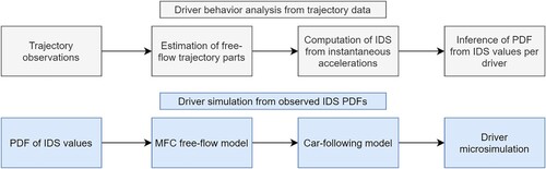
We propose a methodological approach to analyse a driver’s behaviour based on observed vehicle trajectories and reproduce observed driver behaviours in microsimulation. A high-level schematic representation of the proposed framework is illustrated in Figure 1. The upper part refers to the driver behaviour analysis based on observations. The lower part reproduces characterised behaviours in microsimulation. The different components are discussed in the next sections.

Figure 1. High-level schematic representation of the proposed framework. The top part refers to driver behaviour analysis; the lower part to driver behaviour simulation.

2.1. Independent driving style (IDS)

The focus of the proposed driver behaviour analysis lies in unconstrained driving. This is because under such conditions, the drivers are assumed to have the freedom to accelerate according to their attitudes and therefore it is easier to characterise the behavioural differences. However, please note that unconstrained driving does not correspond necessarily to free-flow driving, i.e. travelling at the desired speed without any interactions with other vehicles.

We consider that unconstrained driving is a superset of free-flow conditions, i.e. when the vehicle has a large enough distance from the leading vehicle (if any). As found in the literature, such conditions are found even under highly congested traffic conditions, e.g. during stop and go situations or between traffic oscillations (Laval, Toth, and Zhou 2014; Makridis et al. 2020). Here, we employ a heuristic approach (threshold-based) for the detection of a large enough distance, as discussed later in the paper.

The main challenge in the data analysis part is that there is no explicit information about whether a movement is constrained or unconstrained and therefore this needs to be estimated. The following section describes the suggested approach of this work towards this aspect.

2.1.1. Estimation of unconstrained vehicle movements

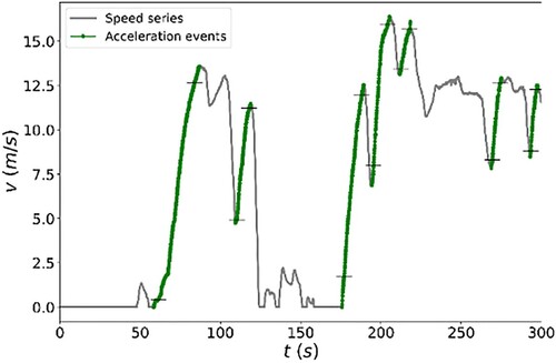
We adopt a simple way to indirectly estimate the unconstrained movement of a vehicle from observations, through the detection of trajectories including sharp-enough accelerations. The idea is that under normal car-following conditions the vehicles are not able to accelerate sharply, as they are bounded by the leading vehicles. Therefore, the essence of detecting unconstrained vehicle movements is correlated with the presence of sharp accelerations in observations.

An acceleration event is considered as a sequence of speed observations starting from a reference speed and ending at a higher one (speed jump of $\mathrm{\Delta }v$). From the observations, it is relatively easy to detect acceleration events by applying a simple local min/max algorithm on the speed time series of the vehicle. If the duration of this acceleration event, namely $w$, is short-enough, while the speed jump $\mathrm{\Delta }v$ is large-enough (indicating sharp acceleration), then the methodology performs the logical assumption that this vehicle is moving unconstrained. The higher the $\mathrm{\Delta }v$, the longer the acceptable $w$ can be.

To define appropriate thresholds for the parameters $\mathrm{\Delta }v$ and $w$, we analyze publicly-available car-following data (Makridis et al. 2021) under the ‘reductio ad absurdum’ logic. In those experiments, vehicles follow their leader in platoon formation. During the driving cycle, the leader randomly accelerates and decelerates sharply, leading to the creation of large-enough inter-vehicle spacing, so that the movement of the following vehicles can be considered unconstrained, i.e. see free-flow pockets (Laval, Toth, and Zhou 2014).

In the above dataset, the parameters $\mathrm{\Delta }v$ and $w$ of the acceleration events are recorded. Based on short, medium, long and very long time durations of the events, we set a threshold value for $\mathrm{\Delta }v$ to the 75th percentile of recorded values and we distinguish constrained versus unconstrained movements. An example of estimated free-flow acceleration events is shown in Figure 2.

Figure 2. Identified sharp acceleration events corresponding to unconstrained vehicle movement in experimental observations.

2.1.2. Acceleration as a measure for driver characterisation

The instantaneous acceleration is often used in the literature to characterise drivers’ style (Berthaume et al. 2018; Hamdar, Mahmassani, and Treiber 2015; Hoogendoorn et al. 2011; Taylor et al. 2015). However, instantaneous acceleration can be misleading for comparative analyses when the drivers use vehicles with very different power capabilities or the observations refer to different traffic conditions or driving environments. To explain this concept, Figure 3 has been derived through modelling from available experimental data and describes the acceleration over the speed domain for one specific vehicle. In particular, in Figure 3 the cyan line depicts the acceleration potential of the vehicle across the whole speed range. The yellow line shows the maximum common acceleration values observed at each given speed, and similar the orange line shows the minimum common deceleration values observed at each given speed for the specific vehicle. These three lines define four regions, namely Regions A, B, C and D.

Figure 3. The unrealistic, feasible and common acceleration-speed domain [model representation from (He et al. 2020; Makridis et al. 2019)] for the vehicle used in the employed experimental campaign (see Section 2.4).

Region C contains the most frequently observed acceleration values. The union between Region B and C describes the domain of plausible values, while Regions A and D include unrealistic acceleration values that the vehicle cannot deliver due to power or other limitations. From the figure, it is possible to understand the unsuitability of acceleration to characterise driving aggressiveness for the following reasons. First, when two vehicles have a significant difference in power capabilities, their acceleration at a given speed is not comparable. Second, a driver adapts to the vehicle's capabilities. Therefore, it is unfair to characterise a driver of a high power car as more aggressively only because the car can produce higher acceleration than conventional ones. Third, the acceleration response of market vehicles is not uniform across their speed range. It is obvious from Figure 3 that the maximum possible acceleration for speeds around $10\text{m}/\text{s}$ (urban) is higher than $4\text{m}/{\text{s}}^2$, while for speeds around $30\text{m}/\text{s}$ (freeway) is around $1\text{m}/{\text{s}}^2$. It is therefore unfair to compare drivers observed with acceleration values measured at high speeds with those measured at low speeds.

To address this problem, in the present work we introduce an acceleration-based metric that is independent from the vehicle power and the current speed. We achieve this in a two-step methodology described in the next sections.

2.1.3. Vehicle-independent acceleration values

Transformation of instantaneous acceleration values to vehicle-independent ones is possible once the vehicle specifications are known. In this case, it is indeed possible to define the maximum possible acceleration that that vehicle can deliver at a given speed and by using this value the acceleration can be described as a rate of the vehicle’s acceleration potential at the given speed.

There are several models of this type in the literature (Fadhloun and Rakha 2020; Makridis et al. 2019; Rakha, Snare, and Dion 2004, 2012). Here, we use the MFC model proposed in Makridis et al. (2019). The employed model has been extended also for electric vehicles that demonstrate different power distribution across speed ranges (He et al. 2020).

Using the MFC model we construct the acceleration capacity function of the vehicle, namely $a_{cp}\left(v\right)$ (i.e. cyan line in Figure 3), where $v$ is the instantaneous speed. It should be noted that $a_{cp}\left(v\right)$ is also a function of the current gear, which is computed based on the work of (Fontaras et al. 2018). Then we express the instantaneous acceleration $a$ as a rate of $a_{cp}\left(v\right)$: (1) $\begin{array}{r}ds=\frac{a}{a_{cp}\left(v\right)}\end{array}$(1) As it can be noted, the $ds$ quantity is related to the acceleration but it is independent of the vehicle's power capabilities. More specifically, the $a_{cp}\left(v\right)$ is the maximum possible acceleration of the vehicle at the given speed $v$. Therefore, if we divide an observed acceleration at that speed by the acceleration potential of the vehicle, the resulted quantity can be considered as vehicle-independent, describing only the driver. For more information, we refer the reader to the MFC model (Makridis et al. 2019). In generalised studies, the reader can use average acceleration potential functions based on average vehicle performance in commercial fleets to avoid the need for knowledge of each vehicle’s specifications.

In the remaining part of the driver analysis, we perform the logical assumption that a driver does not change his/her driving behaviour during a single acceleration event. Therefore, instead of working on instantaneous acceleration, we continue our analysis based on the median acceleration/speed values observed during a detected unconstrained movement. This is a logical assumption that reduced computational complexity and provides invariability to noisy observations (Punzo, Borzacchiello, and Ciuffo 2011).

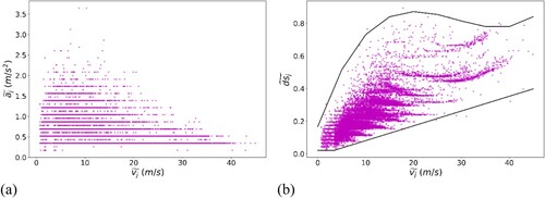
Figure 4 is an intuitive demonstration of this new vehicle-independent metric. The plots refer to naturalistic data from a large pool of drivers (see later the description of the experimental campaign). Each point in Figure 4(a) shows the median acceleration and speed values of an observed unconstrained movement. As expected, the upper boundary of the observed accelerations, i.e. maximum values, are much higher for low speeds than for high speeds due to non-uniform vehicle power dynamics. It is worth noting that there are two reasons why low acceleration values correspond to unconstrained movement and appear in Figure 4(a). First, since the maximum possible acceleration for a vehicle is a function of speed, low acceleration values at high speeds are considered sharp enough from the proposed method. Second, there are different $\mathrm{\Delta }v$ and $w$ thresholds depending on the event duration (see Section 2.1.1) which means that events including low accelerations can be admissible for higher speeds but not for lower ones. Figure 4(b) shows the proposed $ds$ values and speed values. The black lines are piece-wise linear functions used to inscribe the operational domain of all observed values.

Figure 4. Naturalistic data refer to the 20 observed drivers of the experimental campaign used in this work. (a) shows acceleration over speed per movement and (b) the proposed $ds$ values per speed per movement.

2.1.4. Speed-independent acceleration values

We discussed how $ds$ is a vehicle-independent metric but the correlation with speed remains. The observed $ds$ values are lower at low speeds and higher at high speeds, demonstrating the opposite tendency of acceleration values. We employ a simple normalisation process to tackle this issue. First, we derive two piece-wise equations that describe the black lines observed in Figure 4(b), namely $f_{min}\left(v\right)$ and $f_{max}\left(v\right)$. The fitted curves are reported in Appendix Part A for the reproducibility of the proposed study. Second, we express the observed $ds$ values as a rate of the operational domain that $f_{min}$ and $f_{max}$ describe as follows: (2) $\begin{array}{r}ids=\frac{ds\left(v\right)-f_{min}\left(v\right)}{f_{max}\left(v\right)-f_{min}\left(v\right)}\end{array}$(2) where $ids$ is called Independent Driving Style (IDS), $ds$ comes from Eq.1 and $v$ is the observed median speed in an unconstrained movement. For the sake of demonstration in this work, we assume that the $f_{min}\left(v\right)$ and $f_{max}\left(v\right)$ have global validity. In other words, we assume that our pool of drivers is large enough to describe all possible driving behaviours, or our dataset is large enough to capture all possible networks and traffic conditions. Consequently, in a real-world application, the $f_{min}\left(v\right)$ and $f_{max}\left(v\right)$ need to be updated as new observations arrive to describe the drivers’ operational domain properly. 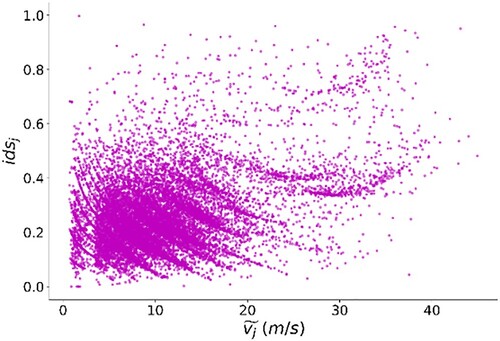Figure 5 shows normalised $ids$ values per speed.

Figure 5. Uniform distribution of IDS values across the whole speed range. Data refer to 20 observed drivers ($\mathit{j}$ denotes the ID of an acceleration event).

2.2. Driver characterisation using distributions of IDS values

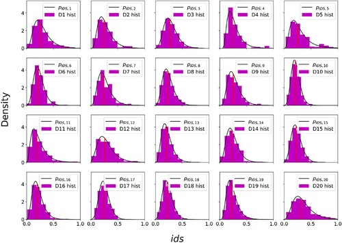
Each observed IDS value corresponds to an observed unconstrained vehicle movement and the main assumption is that this movement can be part of the driver’s fingerprint and characterise him. Assuming enough observations per driver, we can construct the IDS histogram of this driver and then approximate the derived histogram with the probability density function (PDF) to enable analytical comparisons. In this work, we assume and validate (later in the paper) our assumption that driver IDS observations follow a lognormal PDF. Each fitted PDF can be thought of as the driver’s behavioural fingerprint.

2.3. Stochastic microsimulation of observed drivers

Assuming a composed IDS PDF for a driver this section describes how proposed simulation of this driver can be achieved. The IDS PDF is used to randomly select the acceleration of a vehicle in a Monte Carlo fashion. In particular, a randomly sampled number in the [0,1] is thus first defined. Via the PDF the number is translated into a value of IDS and using the following two simple equations (which reverse Equations (1) and (2)) into an acceleration value: (3) $\begin{array}{rl}ds& =ids\cdot \left(f_{max}\left(v\right)-f_{min}\left(v\right)\right)+f_{min}\left(v\right)\end{array}$(3) (4) $\begin{array}{rl}a& =[ds\cdot (f_{max}\left(v\right)-f_{min}\left(v\right))+f_{min}(v_t\left)\right]a_{cp}\left(v\right)\end{array}$(4) It is worth underlying that once the efforts to obtain the IDS PDFs have been made, using the model in combination with traffic simulation becomes extremely simple and lightweight.

2.4. Experimental campaign

To validate the proposed methodology we conducted an experimental campaign in which 20 different drivers using the same vehicle under different driving conditions for 12 months. The vehicle used in the test campaign is a 2.0L diesel C-segment passenger car, equipped with automatic transmission (9 gears), leased for 12 months (during 2016 and 2017). The dataset consists of more than 10.000 km driven by the drivers. During the experimental campaign, the vehicle was assigned to a volunteer driver, who was free to use it as a personal vehicle for approximately 2 weeks without any restriction on the frequency of usage, the driving style, the fuel consumption or the route choice. For additional information on the test campaign, the reader can also refer to the corresponding publication (Pavlovic et al. 2020).

Table 1 provides an overview of the dataset with distance and trips’ time duration per driver. Time duration refers to actual driving time without long pauses. The differences in the number of driven kilometres or hours travelled can be explained by the fact that there was no restriction or guidance on how each driver could use the vehicle. Additionally, this table shows the number of acceleration events detected for each driver, along with the distance in km covered during those events.

Table 1. Basic statistics of the trips per driver.

Driver	Total km	Total hours	Free-flow events number	Events (km)	Driver	Total km	Total hours	Free-flow events number	Events (km)
D1	250	8	715	117	D11	1056	14	420	171
D2	669	9	447	129	D12	119	4	456	55
D3	1973	39	2807	538	D13	1039	21	1401	307
D4	300	4	223	46	D14	1189	20	1009	295
D5	1055	14	482	134	D15	311	8	548	122
D6	45	2	176	20	D16	2581	35	942	405
D7	166	3	151	58	D17	288	7	632	118
D8	442	13	1054	150	D18	183	7	614	77
D9	310	7	619	111	D19	303	6	345	68
D10	174	6	481	71	D20	1424	19	1139	297

It is worth noting that the distance travelled by the 20 drivers is not the same. Therefore, the statistics presented in Table 1 vary among the drivers. Since the main assumption in the paper is that the collected data per driver are enough to accurately describe his driving profile, this difference may affect the generality of the results achieved. Nevertheless, we do not consider this limitation critical for demonstrating the robustness of the proposed approach and additionally we expect that it will disappear in the future with the abundance of in-vehicle (e.g. telematics) or infrastructure (e.g. Bluetooth) sensors that can collect large volumes of personalised driver data.

3. Results

This section presents the results of the proposed methodology to characterise intra- and inter-driver heterogeneity, as well as simulate specific driver profiles.

3.1. Inferring the PDF distribution per driver

In the methodology section IDS was identified as a normalised metric, independent of the speed and the vehicle’s powertrain, suitable to perform an objective comparison between different drivers. The IDS values per driver were derived from the median accelerations observed during the acceleration events derived using the methodology described in Section 2. The derivation of lognormal PDF was assessed using the Kolmogorov–Smirnov (K-S) test, which is a nonparametric statistical test of the equality of one-dimensional probability distributions. K-S is used here as a goodness of fit test to compare the observed histogram with the continuous reference-fitted PDF.

In Figure 6, the empirical distributions of observed IDS values per driver are presented with the y-axis denoting probability density. The lognormal distribution has been indeed mentioned in the literature as suitable for the description of human behaviour. Gualandi and Toscani studied the connection between human behaviour and lognormal distribution also considering cases of modelling drivers in traffic (Gualandi and Toscani 2019). Furthermore, Antoniou et al. (2002) concluded that the aggregation of traffic measurements forms a statistical distribution, which is quite accurately described by a lognormal distribution. The goodness of fit test results based on the K-S method are reported in Appendix Part B. The parameters of the lognormal PDFs for all drivers are given for reference in Appendix Part C.

Figure 6. Histogram of the observed IDS values for each driver along with the fitted lognormal PDF. The vertical red lines denote the location of the median.

3.2. Inter-driver heterogeneity

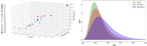
With inter-driver heterogeneity, we refer to the difference in the driving styles among drivers. This heterogeneity is explored through the fitted PDF related to each driver. A visual inspection of the different driving behaviours is already visible in Figure 6. To have a more macroscopic representation of the inter-driver heterogeneity, we perform a semantic categorisation of the 20 drivers into conceptually-perceived driver profiles, i.e. mild, normal or dynamic. We attempt to cluster all drivers in the afore-mentioned generic categories using the simple K-means algorithm (Macqueen 1967). The variables used for the K-means clustering refer to descriptive statistics of the lognormal PDFs. Three features were used for that, one related to the central tendency of the PDF and another two related to the spread of the PDF (25th, 75th percentiles), as they were found performing well in describing the driver categories.

Figure 7(a) presents the results of this grouping in the form of a 3D plot. The axes refer to the median, the 25th and the 75th percentile values. Drivers belonging to the same group are plotted with the same marker, while black points show the clustering centres, which are the representatives of each group. The results are bounded by the small size of the dataset, yet interesting findings can be deduced. One driver (D20) exhibited significant differences from the rest of the drivers, which was also obvious in the visual inspection and constituted a separate group. Figure 7(b) presents the distribution per driver category. As expected, there is a large overlapping area between the different driver categories. An aggressive driver is not expected to drive constantly in an aggressive way, as this is not always allowed, e.g. due to traffic state, weather, mood or other stochastic factors. The distribution of mild drivers shows a higher probability for lower IDS values than normal or aggressive ones. For reference, later in the paper, Drivers with ids 6,7,10,11,13,15,16,18 and 19 are categorised as mild, drivers with ids 1,2,3,4,5,7,9,12 and 17 are categorised as normal and driver with id 20 is considered in the dynamic category.

Figure 7. (a) K-means clustering result presented in a 3D plot, (b) PDFs of the inferred mild, normal and dynamic driver type.

3.3. Intra-driver heterogeneity

Intra-driver heterogeneity refers to the different driving styles that a driver employs under various conditions. This kind of heterogeneity is assessed here since it is a crucial factor potentially affecting the observed variation in traffic-related variables such as headway (L. Li et al. 2020). An idea of the variation in the driving style of a single driver is already taken by observing the fitted PDF. Its wideness visually shows which driver is more consistent with his driving style concerning others.

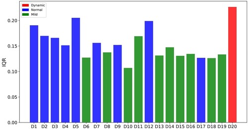
To quantitatively explore the intra-driver heterogeneity, we refer again to descriptive statistics. More specifically, we use a measure of statistical dispersion, the interquartile range (IQR), which is equal to the difference between the 75th and 25th percentiles. Drivers with bigger IQR are considered to have a bigger degree of intra-driver heterogeneity. This heterogeneity is linked only to the different driving behaviours since the vehicle remains the same in all cases. Figure 8 illustrates the IQR values for each driver. Drivers D1, D5, D12 (normal category) and D20 (dynamic category) demonstrate the biggest IQR, and therefore largest intra-driver heterogeneity. Furthermore, as expected most mild drivers demonstrate low intra-driver heterogeneity, i.e. narrow IDS distributions. These quantitative results are aligned with expected empirical behaviours for mild, normal and dynamic drivers.

Figure 8. Bar plot of the IQR of the drivers’ PDFs.

3.4. Simulation of individual driving styles and traffic flow

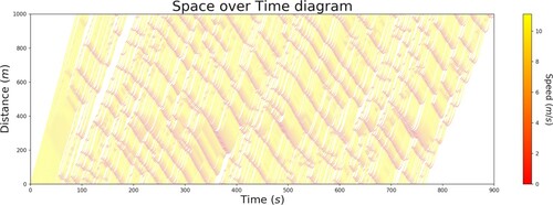
In traffic simulation practice, individual driving styles are commonly simulated through stochasticity in the acceleration parameter of the employed car-following model. However, as already mentioned, the statistical variance of the parameter includes the aggregation of vehicle dynamics, driver aggressiveness and possibly other factors as well. Therefore, upon calibration, it most probably loses its physical meaning as it contributes, together with the other parameters, to resemble a real-world trajectory by overfitting. For simulation of individual driver profiles, we suggest detailed models that introduce an explicit description of vehicle dynamics and driver profile (Fadhloun and Rakha 2020; Makridis et al. 2019). As already mentioned, this work uses the Microsimulation Free-flow aCceleration model (MFC) for this purpose (Makridis et al. 2019). In a previous study by the authors, it was demonstrated how the MFC can be incorporated in car-following models by replacing their free-flow component (Makridis et al. 2020). Results have shown that by adopting a simplified Lagrangian Godunov scheme (Leclercq, Laval, and Chevallier 2007) the MFC can reproduce macroscopically-observed phenomena with the formation and propagation of traffic oscillations in the absence of lane changes that can be explained by the stochastic nature of drivers’ acceleration processes. Moreover, MFC supports the car-following model to reproduce the concave growth pattern of the speed standard deviation for a group of vehicles in car-platoon formation. Figure 9 illustrates the MFC behaviour within the framework of the LWR model. In particular, in this framework, the MFC model replaces the free-flow component of the Newell car-following model (Figure 9). It is worth noting that for the new model, the free-flow part is enabled also under congested conditions, i.e. when the distance from the leading vehicle is large enough, e.g. in oscillations. Therefore this confirms that, although the inference is based on unconstrained driving (including free-flow), the impact of the induced driving heterogeneity appears under both free-flow and congested traffic conditions. It is worth noting that the proposed solution does not influence traffic simulation under equilibrium car-following conditions, i.e. when leader and follower have the same speed moving near equilibrium spacing. This is of course expected since the driving behaviour in this case is mainly affected by the vehicle in front.

Figure 9. Reproduction of empirically-observed traffic oscillations with the MFC-LWR model as shown in (Makridis et al. 2020).

In the present work, instead of using a constant driver behaviour parameter, we sample in real time the driver behaviour parameter from the driver’s derived distribution (PDF). Since the aim of this work is not on traffic oscillations, in this section, we provide validation results only on the new free-flow behaviour of the proposed model. However, it can be expected that the new model can produce oscillations of even more variable amplitudes and frequencies.

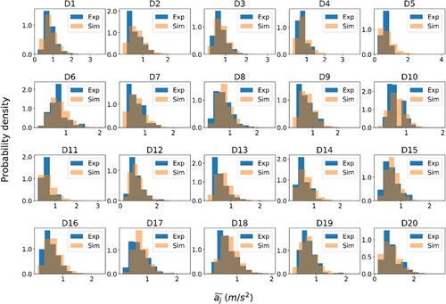
The assessment of the proposed model to simulate different drivers is performed on two levels. First, all the events with observed unconstrained movements from all drivers are considered and simulated, i.e. acceleration from the low speed to the high speed of a certain event. Model-wise, each event is simulated based on a randomly sampled IDS value from the respective PDF of each driver. For each event, we perform 10 simulations, each one with a different random IDS sample. Figure 10 shows the observed and the simulated driver distributions for median acceleration values per unconstrained movement, for all drivers. The results are very promising and it is worth noting that close reproduction of speed and acceleration values per driver can help towards a more accurate simulation of the driver’s energy consumption profile as well.

Figure 10. Median acceleration per event histograms of measured and simulated data.

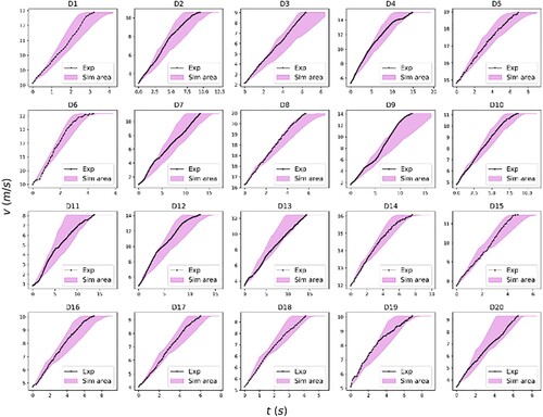
Looking at individual unconstrained movements, for each event of each driver, we perform two simulations, using the 25th and 75th percentiles from the driver’s PDF. Figure 11 shows for an indicative event per driver how empirical accelerations lie within the area inscribed by the two simulations.

Figure 11. An indicative unconstrained movement per driver. For each event, the simulation area with the 25^th and 75th percentile from the driver’s PDF is highlighted.

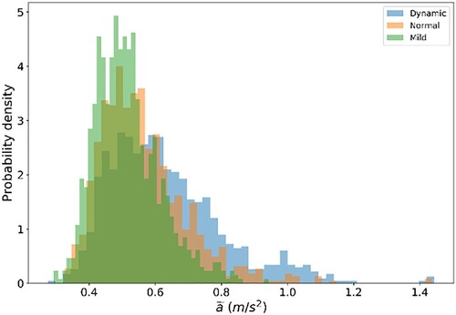
Finally, it is interesting to see how different driver categories appear in simulation. We set up an acceleration scenario with a fixed duration of 90s from 0 to 30 m/s desired speed with the proposed model. If the driver reaches the desired speed before the end of the scenario duration, the same speed is kept for the remaining time. We perform 1000 simulations with randomly selected IDS values from each category’s PDF, i.e. 3000 simulations in total. Figure 12 shows histograms of median accelerations for the simulated event per driver type. One can distinguish the different types of drivers but also the overlapping areas in the respective PDFs, as expected in real-world observations. Finally, looking from a high-level analysis point of view, we see in the majority of the cases, the dynamic driver is faster than the normal (61.5% – cases 1,2,6), and the mild one (70.1% – cases 1,2,3) and the mild driver is slower than that dynamic (70.1% – cases 1,2,3) and the normal one (59.5% – cases 1,3,4).

Figure 12. Histograms of median accelerations of the simulations concerning the three driver types.

The implementation of the proposed framework for individual vehicle trajectory generation is considered outside the present paper’s scope but for indicative applications we refer the reader to a follow-up work by some of the authors (Suarez et al. 2022).

4. Discussion and conclusions

Heterogeneity in the behaviour of human drivers and vehicle dynamics are responsible for the emergence of stochastic patterns in the way vehicles move and interact. On a macroscopic scale, this heterogeneity is responsible for the appearance of various traffic-related phenomena. Thus, accurate modelling and reproduction of individual driving behaviours within microsimulation has lately attracted significant attention in the literature.

Common approaches in traffic simulation takes into account driving heterogeneity assigning randomly sampled values to the models’ acceleration parameter. While this can be sufficient for simulation under synchronised flow conditions in which vehicles proceed with approximately constant speed imposed by the vehicles downstream, there is increasing evidence that this is not the case for when acceleration dynamics play an important role. In this case, indeed the simplified approaches used by car-following models to reproduce acceleration dynamics affects vehicles’ and traffic behaviour not only in free-flow but also in saturated traffic conditions when free-flow pockets arise between the vehicles.

The gaps that currently exist in the literature and the proposed paper aims to tackle can be therefore summarised as follows:

• weak description of free-flow acceleration in microsimulation.

• unfair comparison of drivers’ acceleration behaviour based on instantaneous accelerations.

• challenges to reproduce an observed driver profile in microsimulation.

• challenges to aggregate different driver behaviours in drivers’ categorical representations based solely on trajectory data.

• Challenges in correctly estimating vehicles’ emission.

The present study proposes a novel framework to characterise driver acceleration behaviour based on the analysis of vehicle trajectories. It discusses why instantaneous acceleration can be misleading for comparative analyses when the drivers use vehicles with very different power capabilities or the observations refer to different traffic conditions or driving environments. It proposes a vehicle- and speed-independent acceleration-based metric, namely the Independent Driving Style (IDS). Based on empirical trajectory data from 20 drivers, it studies distributions of IDS values per driver and proposes a concrete way of stochastic driver simulation based on IDS probability density functions.

The contributions of this paper can be therefore summarised as follows:

• it clarifies the role of instantaneous acceleration on driving behaviour representation and comparison among drivers.

• it introduces a vehicle- and speed-independent indicator, (IDS) to describe the driver acceleration behaviour.

• it demonstrates the capability to use the IDS for the characterisation of individual drivers or driver categories, i.e. mild, normal, dynamic.

• it allows an accurate representation of observed individual driver profiles in microsimulation.

Although the employed driver dataset is among the largest publically available ones in its high measurement frequency, it is still rather small to describe all possible driver profiles under real-world conditions. This poses limitations on the proposed framework and make the present results preliminary. More specifically, it is still not clear the amount of individual driver data needed for a complete PDF characterisation. Additionally, domain descriptive piece-wise linear functions, $f_{min}$ and $f_{\text{max}}$, introduced in Section 2.1.4 will change as more data will be used. Moreover, semantic categorisation of drivers is used only indicatively to highlight the potential of the proposed framework. Finally, an important role might be played by the gear shifting strategy of the driver (for manual gearboxes) as described in the original MFC model (Makridis et al. 2019). However, this factor is considered homogeneous in the present study since the vehicle used in the experimental campaign was equipped with automatic transmission. It has to be said that with the fast increasing penetration rate of automatic gearboxes, the role of the gear shifting strategy may become limited.

Future work will assess through large-scale experimental data, the capability of the proposed study to describe and differentiate the behavioural differences of automated driver assistance systems, as well as compare their behaviour with human drivers. Furthermore, another metric that is considered in the literature for modelling heterogeneity is the different target spacing per driver at equilibrium conditions, as shown in a methodological development with Newell’s model (Laval and Leclercq 2010). Since this factor can be especially important in the case of synchronised flow, combining it with the approach proposed in the present study can be considered an interesting follow-up of the present research.

Acknowledgements

The views expressed are purely those of the authors and may not, under any circumstances, be regarded as an official position of the European Commission. The work by A. Anesiadou has been carried out at the European Commission Joint Research Centre. The authors are grateful to Vincenzo Arcidiacono for the help regarding the CO2MPAS gear identification tool and to Jelica Pavlovic and Kostis Anagnostopoulos for the help regarding the pre-processing of the experimental data.

Disclosure statement

No potential conflict of interest was reported by the author(s).

Additional information

Funding

This research has been funded by the Joint Research Centre of the European Commission.

Notes

1 https://pypi.org/project/co2mpas-driver/

2 https://www.aimsun.com/knowledge-base/mfc-and-battery-consumption-model/

Appendix

Part A – Fitted curves defining the operational domain in median DS-median speed space

Table A1. Characteristics of fitted curves along with the special conditions for each one.

Curve	Polynomial curves	Special conditions
$f_{\text{min}}$	$f_{\text{min}}\left(\tilde{v}\right)=0.009\cdot \tilde{v}-0.009$	$f_{\text{min}}\left(\tilde{v}\right)\ge Min{\widetilde{ds}}_{exp}$
$f_{\text{max}}$	$f_{\text{max}}\left(\tilde{v}\right)=3.70\cdot {10}^{-5}{\tilde{v}}^3-0.003{\tilde{v}}^2+0.084\cdot \tilde{v}+0.167$

Where $Min{\widetilde{ds}}_{exp}$ is the minimum observed median $ds$ value equal to 0.021, $\tilde{v}$ is the median speed value.

Part B – Goodness of fit K-S test of all drivers

Table A2 shows the results of the goodness of fit K-S test of all the $p_{IDS,i}$ functions. In all driver cases, the test statistic value was smaller than the critical value ($\text{D}<\text{Critical}$) which allows us not to reject the null hypothesis and accept, with a 1% level of significance, that all $id{s}_{i,j}$ distributions can be represented by the inferred $p_{IDS,i}s$. Additionally, the resulting p-values were larger than the significance level (p-values ≫significance level), providing more evidence on not rejecting the null hypothesis.

Table A2. The goodness of fit test results based on the K-S method.

Driver	Critical value	D statistic	p-value	Driver	Critical value	D statistic	p-value
D1	0.061	0.037	0.280	D11	0.080	0.019	0.999
D2	0.077	0.032	0.739	D12	0.076	0.036	0.596
D3	0.031	0.013	0.710	D13	0.043	0.019	0.662
D4	0.109	0.042	0.822	D14	0.051	0.032	0.264
D5	0.074	0.040	0.404	D15	0.070	0.023	0.928
D6	0.123	0.067	0.391	D16	0.053	0.035	0.188
D7	0.132	0.048	0.870	D17	0.065	0.026	0.768
D8	0.050	0.015	0.969	D18	0.066	0.024	0.859
D9	0.065	0.036	0.396	D19	0.088	0.035	0.782
D10	0.074	0.039	0.435	D20	0.048	0.022	0.662

Part C – Parameters of the lognormal PDFs of all drivers

A three-parameter lognormal PDF $p_{IDS,i}$ (Singh 1998), with $i$ being the driver id, is fitted at each one of them and shown as a black curve in the figure. The first parameter (shape) denotes the general form-shape of the distribution and is also equal to the standard deviation of the $ln\left(id{s}_{i,j}\text{--}location\right)$, the second one (location) reveals the shift on the x-axis, representing a lower bound and the last one if combined with the shift parameter (scale + location) expresses the median of the $p_{IDS,i}$. For completion, Appendix B includes the parameters of the inferred $p_{IDS,i}$s. The location of the median for each $p_{IDS,i}$ is denoted with a vertical red line in the figure.

Table A3 presents the lognormal parameters which actually characterise the drivers. One can see that in most cases location parameters are slightly negative which means there is a tiny probability that the PDF takes negative values (more specifically, among all probabilities for an $p_{IDS,i}$ to get values smaller or equal to zero, the biggest one is 0.17%). At this stage we also note that those parameters do mathematically reconstruct each $p_{IDS,i}$, however, they do not directly reveal meaningful information for the lognormal itself, apart from the location shift. Therefore, descriptive statistics of each $p_{IDS,i}$ are used to analyse further the drivers’ characteristics.

Table A3. Parameters of the lognormal PDFs.

Driver	shape	location	scale	Driver	shape	location	scale
D1	0.448	−0.051	0.311	D11	0.560	−0.025	0.219
D2	0.456	−0.030	0.272	D12	0.383	−0.124	0.381
D3	0.312	−0.120	0.392	D13	0.355	−0.067	0.272
D4	0.529	0.031	0.208	D14	0.334	−0.099	0.324
D5	0.575	−0.011	0.258	D15	0.238	−0.182	0.405
D6	0.265	−0.132	0.353	D16	0.369	−0.068	0.267
D7	0.382	−0.064	0.300	D17	0.207	−0.211	0.452
D8	0.298	−0.113	0.340	D18	0.228	−0.189	0.409
D9	0.378	−0.046	0.295	D19	0.400	−0.026	0.244
D10	0.211	−0.166	0.375	D20	0.410	−0.089	0.405

References

- Aghabayk, K., N. Forouzideh, and W. Young. 2013a. “Exploring a Local Linear Model Tree Approach to Car-Following.” Computer-Aided Civil and Infrastructure Engineering 28: 581–593. doi:10.1111/mice.12011.
- Aghabayk, K., M. Sarvi, N. Forouzideh, and W. Young. 2013b. “New Car-Following Model Considering Impacts of Multiple Lead Vehicle Types.” Transportation Research Record: Journal of the Transportation Research Board 2390: 131–137. doi:10.3141/2390-14.
- Al Haddad, C., and C. Antoniou. 2022. “A Data–Information–Knowledge Cycle for Modeling Driving Behavior.” Transportation Research Part F: Traffic Psychology and Behaviour 85: 83–102. doi:10.1016/j.trf.2021.12.017.
- Alhariqi, A., Z. Gu, and M. Saberi. 2022. “Calibration of the Intelligent Driver Model (IDM) with Adaptive Parameters for Mixed Autonomy Traffic Using Experimental Trajectory Data.” Transportmetrica B: Transport Dynamics 10: 421–440. doi:10.1080/21680566.2021.2007813.
- Antoniou, I., V. V. Ivanov, Valery V Ivanov, and P. V. Zrelov. 2002. “On the Log-Normal Distribution of Network Traffic.” Physica D: Nonlinear Phenomena 167: 72–85. doi:10.1016/S0167-2789(02)00431-1.
- Berthaume, A. L., R. M. James, B. E. Hammit, C. Foreman, and C. L. Melson. 2018. “Variations in Driver Behavior: An Analysis of Car-Following Behavior Heterogeneity as a Function of Road Type and Traffic Condition.” Transportation Research Record: Journal of the Transportation Research Board 2672: 31–44. doi:10.1177/0361198118798713.
- Calvert, S. C., and B. van Arem. 2020. “A Generic Multi-level Framework for Microscopic Traffic Simulation with Automated Vehicles in Mixed Traffic.” Transportation Research Part C: Emerging Technologies 110: 291–311. doi:10.1016/j.trc.2019.11.019.
- Chen, D., S. Ahn, J. Laval, and Z. Zheng. 2014. “On the Periodicity of Traffic Oscillations and Capacity Drop: The Role of Driver Characteristics.” Transportation Research Part B: Methodological 59: 117–136. doi:10.1016/j.trb.2013.11.005.
- Ciuffo, B., M. Makridis, T. Toledo, and G. Fontaras. 2018. “Capability of Current Car-Following Models to Reproduce Vehicle Free-Flow Acceleration Dynamics.” IEEE Transactions on Intelligent Transportation Systems 19: 3594–3603. doi:10.1109/TITS.2018.2866271.
- Fadhloun, K., and H. Rakha. 2020. “A Novel Vehicle Dynamics and Human Behavior Car-following Model: Model Development and Preliminary Testing.” International Journal of Transportation Science and Technology 9: 14–28. doi:10.1016/j.ijtst.2019.05.004.
- Fontaras, G., V. Valverde, V. Arcidiacono, S. Tsiakmakis, K. Anagnostopoulos, D. Komnos, J. Pavlovic, and B. Ciuffo. 2018. “The Development and Validation of a Vehicle Simulator for the Introduction of Worldwide Harmonized Test Protocol in the European Light Duty Vehicle CO2 Certification Process.” Applied Energy 226: 784–796. doi:10.1016/j.apenergy.2018.06.009.
- Gualandi, S., and G. Toscani. 2019. “Human Behavior and Lognormal Distribution. A Kinetic Description.” Mathematical Models and Methods in Applied Sciences 29: 717–753. doi:10.1142/S0218202519400049.
- Hamdar, S. H., H. S. Mahmassani, and M. Treiber. 2015. “From Behavioral Psychology to Acceleration Modeling: Calibration, Validation, and Exploration of Drivers’ Cognitive and Safety Parameters in a Risk-taking Environment.” Transportation Research Part B: Methodological 78: 32–53. doi:10.1016/j.trb.2015.03.011.
- He, Y., M. Makridis, K. Mattas, G. Fontaras, B. Ciuffo, and H. Xu. 2020. “Introducing Electrified Vehicle Dynamics in Traffic Simulation.” Transportation Research Record: Journal of the Transportation Research Board 2674: 776–791. doi:10.1177/0361198120931842.
- Hoogendoorn, R. G., S. P. Hoogendoorn, K. A. Brookhuis, and W. Daamen. 2011. “Adaptation Longitudinal Driving Behavior, Mental Workload, and Psycho-Spacing Models in Fog.” Transportation Research Record: Journal of the Transportation Research Board 2249: 20–28. doi:10.3141/2249-04.
- Huang, Y.-X., R. Jiang, H. Zhang, M.-B. Hu, J.-F. Tian, B. Jia, and Z.-Y. Gao. 2018. “Experimental Study and Modeling of Car-following Behavior Under High Speed Situation.” Transportation Research Part C: Emerging Technologies 97: 194–215. doi:10.1016/j.trc.2018.10.022.
- Jiang, R., M.-B. Hu, H. M. Zhang, Z.-Y. Gao, B. Jia, and Q.-S. Wu. 2015. “On Some Experimental Features of Car-following Behavior and How to Model Them.” Transportation Research Part B: Methodological 80: 338–354. doi:10.1016/j.trb.2015.08.003.
- Kilpeläinen, M., and H. Summala. 2007. “Effects of Weather and Weather Forecasts on Driver Behaviour.” Transportation Research Part F: Traffic Psychology and Behaviour 10: 288–299. doi:10.1016/j.trf.2006.11.002.
- Lajunen, T., D. Parker, and H. Summala. 1999. “Does Traffic Congestion Increase Driver Aggression?” Transportation Research Part F: Traffic Psychology and Behaviour 2: 225–236. doi:10.1016/S1369-8478(00)00003-6.
- Laval, J. A., and L. Leclercq. 2010. “A Mechanism to Describe the Formation and Propagation of Stop-and-go Waves in Congested Freeway Traffic.” Philosophical Transactions of the Royal Society A: Mathematical, Physical and Engineering Sciences 368: 4519–4541. doi:10.1098/rsta.2010.0138.
- Laval, J. A., C. S. Toth, and Y. Zhou. 2014. “A Parsimonious Model for the Formation of Oscillations in car-Following Models.” Transportation Research Part B: Methodological 70: 228–238. doi:10.1016/j.trb.2014.09.004.
- Leclercq, L., J. A. Laval, and E. Chevallier. 2007. “The Lagrangian Coordinates and What it Means for First Order Traffic Flow Models.” Presented at the International Symposium on Transportation and Traffic Theory.
- Li, L., R. Jiang, Z. He, X. (Michael) Chen, and X. Zhou. 2020. “Trajectory Data-based Traffic Flow Studies: A Revisit.” Transportation Research Part C: Emerging Technologies 114: 225–240. doi:10.1016/j.trc.2020.02.016.
- Li, L., Y. Li, and D. Ni. 2021. “Incorporating Human Factors into LCM Using Fuzzy TCI Model.” Transportmetrica B: Transport Dynamics 9: 198–218. doi:10.1080/21680566.2020.1837033.
- Li, T., D. Ngoduy, F. Hui, and X. Zhao. 2020. “A Car-following Model to Assess the Impact of V2V Messages on Traffic Dynamics.” Transportmetrica B: Transport Dynamics 8: 150–165. doi:10.1080/21680566.2020.1728591.
- Li, G., Z. Yang, Y. Pan, and J. Ma. 2022. “Analysing and Modelling of Discretionary Lane Change Duration Considering Driver Heterogeneity.” Transportmetrica B: Transport Dynamics, 1–18. doi:10.1080/21680566.2022.2067599.
- Macqueen, J. 1967. Some Methods for Classification and Analysis of Multivariate Observations 5.1, 17.
- Makridis, M., G. Fontaras, B. Ciuffo, and K. Mattas. 2019. “MFC Free-Flow Model: Introducing Vehicle Dynamics in Microsimulation.” Transportation Research Record, 036119811983851. doi:10.1177/0361198119838515.
- Makridis, M., L. Leclercq, B. Ciuffo, G. Fontaras, and K. Mattas. 2020. “Formalizing the Heterogeneity of the Vehicle-driver System to Reproduce Traffic Oscillations.” Transportation Research Part C: Emerging Technologies 120: 102803.
- Makridis, M., K. Mattas, A. Anesiadou, and B. Ciuffo. 2021. “OpenACC. An Open Database of car-Following Experiments to Study the Properties of Commercial ACC Systems.” Transportation Research Part C: Emerging Technologies 125: 103047.
- Nagahama, A., D. Yanagisawa, and K. Nishinari. 2020. “Car-following Characteristics of Various Vehicle Types in Respective Driving Phases.” Transportmetrica B: Transport Dynamics 8: 22–48. doi:10.1080/21680566.2019.1710002.
- Ngoduy, D., S. Lee, M. Treiber, M. Keyvan-Ekbatani, and H. L. Vu. 2019. “Langevin Method for a Continuous Stochastic Car-Following Model and its Stability Conditions.” Transportation Research Part C: Emerging Technologies 105: 599–610. doi:10.1016/j.trc.2019.06.005.
- Ossen, S., and S. P. Hoogendoorn. 2011. “Heterogeneity in Car-following Behavior: Theory and Empirics.” Transportation Research Part C: Emerging Technologies, Emerging Theories in Traffic and Transportation and Methods for Transportation Planning and Operations 19: 182–195. doi:10.1016/j.trc.2010.05.006.
- Özkan, T., T. Lajunen, J.El. Chliaoutakis, D. Parker, and H. Summala. 2006. “Cross-cultural Differences in Driving Behaviours: A Comparison of six Countries.” Transportation Research Part F: Traffic Psychology and Behaviour 9: 227–242. doi:10.1016/j.trf.2006.01.002.
- Pavlovic, J., G. Fontaras, M. Ktistakis, K. Anagnostopoulos, D. Komnos, B. Ciuffo, M. Clairotte, and V. Valverde. 2020. “Understanding the Origins and Variability of the Fuel Consumption Gap: Lessons Learned from Laboratory Tests and a Real-driving Campaign.” Environmental Sciences Europe 32: 53. doi:10.1186/s12302-020-00338-1.
- Punzo, V., M. T. Borzacchiello, and B. Ciuffo. 2011. “On the Assessment of Vehicle Trajectory Data Accuracy and Application to the Next Generation SIMulation (NGSIM) Program Data.” Transportation Research Part C: Emerging Technologies 19: 1243–1262. doi:10.1016/j.trc.2010.12.007.
- Raju, N., S. Arkatkar, S. Easa, and G. Joshi. 2022. “Customizing the Following Behavior Models to Mimic the Weak Lane Based Mixed Traffic Conditions.” Transportmetrica B: Transport Dynamics 10: 20–47. doi:10.1080/21680566.2021.1954562.
- Rakha, H. A., K. Ahn, W. Faris, and K. S. Moran. 2012. “Simple Vehicle Powertrain Model for Modeling Intelligent Vehicle Applications.” IEEE Transactions on Intelligent Transportation Systems 13: 770–780. doi:10.1109/TITS.2012.2188517.
- Rakha, H., M. Snare, and F. Dion. 2004. “Vehicle Dynamics Model for Estimating Maximum Light-Duty Vehicle Acceleration Levels.” Transportation Research Record: Journal of the Transportation Research Board 1883: 40–49. doi:10.3141/1883-05.
- Saifuzzaman, M., Z. Zheng, Md.M. Haque, and S. Washington. 2017. “Understanding the Mechanism of Traffic Hysteresis and Traffic Oscillations Through the Change in Task Difficulty Level.” Transportation Research Part B: Methodological 105: 523–538. doi:10.1016/j.trb.2017.09.023.
- Singh, V. P. 1998. “Three-Parameter Lognormal Distribution.” In Entropy-Based Parameter Estimation in Hydrology, 82–107. Dordrecht: Springer Netherlands. doi:10.1007/978-94-017-1431-0_7
- Suarez, J., M. Makridis, A. Anesiadou, D. Komnos, B. Ciuffo, and G. Fontaras. 2022. “Benchmarking the Driver Acceleration Impact on Vehicle Energy Consumption and CO2 Emissions.” Transportation Research Part D: Transport and Environment 107: 103282. doi:10.1016/j.trd.2022.103282.
- Taylor, J., X. Zhou, N. M. Rouphail, and R. J. Porter. 2015. “Method for Investigating Intradriver Heterogeneity Using Vehicle Trajectory Data: A Dynamic Time Warping Approach.” Transportation Research Part B: Methodological 73: 59–80. doi:10.1016/j.trb.2014.12.009.
- Treiber, M., and A. Kesting. 2013. Traffic Flow Dynamics. Springer Berlin Heidelberg, Berlin, Heidelberg. doi:10.1007/978-3-642-32460-4
- Treiber, M., A. Kesting, and D. Helbing. 2006. “Delays, Inaccuracies and Anticipation in Microscopic Traffic Models.” Physica A: Statistical Mechanics and its Applications 360: 71–88. doi:10.1016/j.physa.2005.05.001.
- Underwood, G., P. Chapman, S. Wright, and D. Crundall. 1999. “Anger While Driving.” Transportation Research Part F: Traffic Psychology and Behaviour 2: 55–68. doi:10.1016/S1369-8478(99)00006-6.
- Wang, H., W. Wang, J. Chen, and M. Jing. 2010. “Using Trajectory Data to Analyze Intradriver Heterogeneity in Car-Following.” Transportation Research Record: Journal of the Transportation Research Board 2188: 85–95. doi:10.3141/2188-10.
- Yagil, D. 1998. “Gender and Age-related Differences in Attitudes Toward Traffic Laws and Traffic Violations.” Transportation Research Part F: Traffic Psychology and Behaviour 1: 123–135. doi:10.1016/S1369-8478(98)00010-2.
- Yuan, K., J. Laval, V. L. Knoop, R. Jiang, and S. P. Hoogendoorn. 2019. “A Geometric Brownian Motion Car-following Model: Towards a Better Understanding of Capacity Drop.” Transportmetrica B: Transport Dynamics 7: 915–927. doi:10.1080/21680566.2018.1518169.
- Zhao, X., Z. Wang, Z. Xu, Y. Wang, X. Li, and X. Qu. 2020. “Field Experiments on Longitudinal Characteristics of Human Driver Behavior Following an Autonomous Vehicle.” Transportation Research Part C: Emerging Technologies 114: 205–224. doi:10.1016/j.trc.2020.02.018.
- Zheng, Z., S. Ahn, D. Chen, and J. Laval. 2011. “Freeway Traffic Oscillations: Microscopic Analysis of Formations and Propagations Using Wavelet Transform.” Transportation Research Part B: Methodological 45: 1378–1388. doi:10.1016/j.trb.2011.05.012.