On the existence and uniqueness properties of the Hoogendoorn–Bovy pedestrian flow model

Abstract

This study addresses the existence and uniqueness of solutions to the Hoogendoorn–Bovy (HB) pedestrian flow model, which describes the dynamic user-optimal pedestrian flow assignment problem in continuous space and time. The HB model consists of a forward conservation law (CL) equation that governs density and a backward Hamilton–Jacobi–Bellman (HJB) equation that contains a maximum admissible speed constraint (MASC), in which the flow direction is determined by the path-choice strategy. The existence and uniqueness of solutions are significantly more difficult to determine when the HJB equation contains an MASC; however, we prove that the HB model can be formulated as a forward CL equation and backward Hamilton–Jacobi (HJ) equation in which the MASC is non-binding if suitable model parameters are selected. This model is formulated as a fixed-point problem upon the simultaneous satisfaction of both equations. To verify the existence and uniqueness results, we first demonstrate the existence and uniqueness of the solutions to the CL and HJ equations, and then show that the coupled HB model is well-posed and has a unique solution. A numerical example is presented to illustrate the properties of the HB model.

Keywords:

• Pedestrian flow
• path-choice
• dynamic continuum model
• existence
• uniqueness

1. Introduction

Dynamic macroscopic pedestrian-flow modelling has received considerable attention in recent decades (Taherifar et al. 2019; Aghamohammadi and Laval 2020; Lin, Zhang, and Hang 2022). The continuum modelling approach has been widely used to study these problems. There are two major components in dynamic macroscopic pedestrian-flow models. The first is a description of the macroscopic characteristics of pedestrian speed, density, and flow (Morrall, Ratnayake, and Seneviratne 1991; Lam, Morrall, and Ho 1995; Lam, Cheung, and Lam 1999; Wong et al. 2010; Xie et al. 2013; Xie and Wong 2015). The second is the route-choice strategy (Hughes 2002; Huang et al. 2009; Frejinger, Bierlaire, and Ben-Akiva 2009; Fosgerau, Frejinger, and Karlstrom 2013; Hoogendoorn and Bovy 2004b; Mai, Fosgerau, and Frejinger 2015), which describes the decision-making process performed by pedestrians to identify the optimal path between an origin and a destination. An important feature of a route-choice problem is a dynamic user equilibrium (DUE) (or dynamic user-optimal (DUO)) problem, which can be divided into two types: (1) the reactive dynamic user-optimal (RDUO) problem, in which pedestrians choose their route in a reactive manner based on instantaneous information, to minimize their instantaneous total walking cost (Hughes 2002; Huang et al. 2009; Yang et al. 2019); and (2) the predictive dynamic user-optimal (PDUO) problem, in which pedestrians are assumed to have perfect information regarding the modelled domain and can choose their route to minimize their actual total walking cost (Hoogendoorn and Bovy 2004a, 2004b).

Many empirical studies (such as experimental or field observation studies) contingent on an assumption regarding the path choice for movement from one place to another (i.e. the DUE principle) have been based on the above-mentioned theoretical studies. Asano, Iryo, and Kuwahara (2010) collected experimental data to validate their pedestrian simulation model that described the anticipatory behaviour of pedestrians and their macroscopic route choice, in which a pedestrian chose a route that satisfied the dynamic user-optimal (DUO) principle. They also conducted an observational survey in a railway station to validate this route choice behaviour. Gao et al. (2014) conducted experiments to collect data for a meeting room with two exits, which were used to calibrate and validate their integrated macroscopic–microscopic approach to simulate the escape process, in which the DUO criterion was formulated to describe pedestrian exit/route choice behaviour. Crociani and Laemmel (2016) collected two datasets at the Technical University Berlin, which were used to support pedestrians' route choice that satisfied either a DUE or a Nash equilibrium adopted in their simulation approach to multi-destination pedestrian crowds in complex environments. In Germany, the dynamic route choice behaviour was tested using two datasets. The first dataset was extracted from a bidirectional flow experiment in which two groups of pedestrians crossed each other with an intersection angle of 180 degree (Plaue et al. 2011), and the second dataset described two groups of pedestrians crossed at an intersection angle of 90 degrees (Plaue et al. 2012).

Confirmation of the existence of solutions is a fundamental challenge to solving both types of DUE problems, and a proof that solutions exist must be obtained prior to performing computations. Han, Friesz, and Yao (2013) showed that a solution existed for the simultaneous route-and-departure choice DUE problem. The existence of continuous-time, system-optimal, and user-optimal traffic flows on a road network is also shown in Bressan and Han (2013). However, a detailed analysis of the existence and uniqueness of solutions to the PDUO/RDUO problem has not been reported, and literature studies have been limited to discussions on model formulation and numerical simulation (Huang et al. 2009; Du et al. 2013; Yang et al. 2019, 2022).

The HB pedestrian flow model (Hoogendoorn and Bovy 2004a, 2004b) was developed to study user-optimal dynamic traffic assignment problems in continuous time and space, and has been widely cited in pedestrian modelling studies ($>1000$ citations since 2004, according to ISI Web of Science). Most of these citations have been in the areas of transportation, engineering and computer science, but there have also been a significant number of citations in a wide variety of other fields. It is therefore very important to identify whether there are solutions to the HB model, and if so, to determine the uniqueness of these solutions.

In the HB model, pedestrians cannot improve their experienced utility (e.g. their experienced or actual walking cost, as opposed to their instantaneous walking costs) by unilaterally changing their path choice, and the model allows pedestrians to choose their routes from an infinite set of paths (Hoogendoorn and Bovy 2004b). The model assumes that pedestrians have perfect information regarding future traffic conditions, which they use to choose a route that minimizes their actual walking cost; thus, this route-choice behaviour is represented as a PDUO problem. This model consists of a forward conservation law (CL) equation and a backward Hamilton–Jacobi–Bellman (HJB) equation, where the latter contains a maximum admissible speed constraint (MASC). There is no analytical solution for this highly coupled model in most cases. In this study, we find that for weight parameters satisfying certain conditions, pedestrians' speed can be shown to be consistently less than the maximum allowed speed. We can then obtain an equivalent equation for the HB model, which consists of a forward CL equation and a backward Hamilton–Jacobi (HJ) equation, but which also contains a non-binding MASC. This assists us to prove the existence and uniqueness of solutions to this HB model.

Conservation laws (e.g. conservation of mass, energy, or momentum laws) can be used to represent many fundamental physical phenomena, and it is therefore important to find analytical and numerical solutions for them. Typically, there are no classical solutions to the CL equation, due to its discontinuities; instead, weak solutions have been derived and have been fundamental to the development and analysis of the CL equation and related numerical methods (Lax 1954). Another mathematical difficulty is that weak solutions are generally non-unique, which means that entropy conditions must be imposed to select a physically correct weak solution (Lax 1971).

In the current study, we focus on a linear CL equation, which also develops discontinuities in its linear coefficients, such that it is unclear whether this equation has unique solutions. Several papers have addressed this issue. Bouchut and James (1998) considered the one-dimensional linear transport equation with a bounded but possibly discontinuous coefficient. They found that a solution exists when the coefficient is piecewise continuous, and that unique and general stability results exist for backward Lipschitz solutions and forward measure solutions when the coefficient satisfies a one-sided Lipschitz condition. Tadmor (1991) showed that the linear transport equation has a unique Lipschitz continuous solution when the coefficient is uniformly bounded and satisfies a one-sided Lipschitz condition, and also showed that the solution satisfies $L^1$ stability. These and other studies have required the initial condition to be locally Lipschitz (Conway 1967; Tadmor 1991; Dolcetta and Perthame 1996; Bouchut and James 1998). In contrast, Petrova and Popov (1999) introduced an entropy condition that selects a unique weak solution for any continuous initial condition, and provided a complete existence-uniqueness theory for such cases.

In physics, the HJ equation is an alternative formulation of classical mechanics, which is particularly useful for identifying the conserved quantities of mechanical systems. The HJB equation is a special class of HJ equation that is crucial for analysing continuous/differential dynamic game and control theory problems. HJ equations do not always have classical solutions, even if the Hamiltonian and initial/boundary conditions are smooth. Thus, the HJ equation is typically solved by searching for viscosity solutions (Crandall and Lions 1983) that are Lipschitz continuous but may have discontinuities in their first derivatives. Several papers have discussed the existence and uniqueness of solutions to HJ equations. Crandall and Lions (1983) established the existence, uniqueness, and stability of viscosity solutions for certain classes of HJ equation. Lions (1982) extended these existence results to more general HJ equation. Crandall, Evans, and Lions (1984) introduced several equivalent formulations for a viscosity solution, examined two of these equivalent criteria in detail, and demonstrated their strength by using them to prove several new results and to reprove various known results in a simpler manner. Fathi (2011) studied the existence of $C^1$ critical sub-solutions of the HJ equation, whereas Sánchez-Morgado et al. (2012) studied the physical solutions of the HJ equation. Existence and uniqueness results have also been obtained by several other authors (e.g. Fleming 1969; Friedman and Hopf 1973).

As outlined above, there have been many studies in recent years to identify and determine the uniqueness of solutions to the conservation law (CL) and to the Hamilton–Jacobi (HJ) equation. In this study, we use suitable parameters to identify and determine the uniqueness of a solution to the HB model. First, we separately consider the existence and uniqueness properties of solutions to the CL and HJ equations. We then focus on a coupled system of CL and HJ equations. This coupling, especially its forward (for the CL equation) and backward (for the HJ equation) nature, makes the analysis of the existence and uniqueness properties of these equations highly challenging.

The findings from this paper provide a solid foundation for understanding the analytical properties of the HB model, which will be useful for researchers who implement this model to solve real-world problems, as it provides insight into the solution properties under different combinations of model parameters. This will enhance user confidence in the existence of a solution and ease user concern about the possibility of multiple solutions under specific conditions. Users will therefore more fully comprehend the limitations and applications of the method for solving real-world problems.

The remainder of this paper is organized as follows. The HB model is described in the next section. In Section 3, we demonstrate the existence and uniqueness of the solution to the HB model. In Section 4, a numerical example is used to demonstrate the effectiveness of the model and justify the exclusion of the minimum value constraint in the analysis. Our conclusions are presented in Section 5.

2. The HB model

In this section, we introduce the formulation of the HB model. First, before discussing the modelling process, we present in Subsection 2.1 the notation and definitions used in the remainder of the paper. In Subsections 2.2–2.3, we introduce the problem formulation and modelling assumptions. In Subsection 2.4, we give the complete model formulation of the original HB model. In Subsection 2.5, we demonstrate that the original HB model can be simplified using suitable parameters, such that the MASC can be ignored.

2.1. Notation and definition

The model region is denoted by $\mathrm{\Omega }\subset R^2$ in which the pedestrians move. Let $O\subset \mathrm{\Omega }$ be the origin area in which the pedestrian enters the model region and $D\subset \mathrm{\Omega }$ be the destination in which the pedestrian leaves the model region, where both the origin and destination are assumed to be closed sets and pedestrian can use any point in the origin/destination area to enter/exit the model region. Let $B\subset \mathrm{\Omega }$ be an obstruction where pedestrians are not allowed to enter and around which they must move while walking to their destination. Let ${\mathrm{\Gamma }}_i$ be the outer boundary of the region Ω, ${\mathrm{\Gamma }}_b$ be the obstruction boundary, and ${\mathrm{\Gamma }}_d$ be the destination boundary. In this study, Ω is assumed to be a bounded set of $R^2$ with a piecewise regular boundary.

The continuum modelling approach is used to describe pedestrian flow; thus, a feasible trajectory for pedestrian movement in the model region can be described by a continuous mathematical function with respect to continuous time t, defined as (1) ${\mathit{x}}_{[t,\overline{t}]}=\{x(s)=(x_1(s),x_2(s))\in \mathrm{\Omega }|t\le s\le \overline{t},\mathit{x}(s)\notin B\}$(1) where t is the departure time and $\overline{t}$ is the terminal time. A pedestrian walks from origin $O\subset \mathrm{\Omega }$ to destination $D\subset \mathrm{\Omega }$. A feasible trajectory should satisfy $\mathit{x}(t)\in O$. If $\mathit{x}(\overline{t})$ is in destination D, then $\overline{t}$ is the time at which the pedestrian arrives at the destination; otherwise, $\overline{t}$ is the end of the time period under consideration.

In the continuum model, a trajectory is assumed to be a differentiable function of t; thus, a velocity exists and is finite. The velocity ${\mathit{v}}_{[t,\overline{t}]}$ along the trajectory ${\mathit{x}}_{[t,\overline{t}]}$ can be defined by (2) ${\mathit{v}}_{[t,\overline{t}]}=\{\mathit{v}(s)\in \mathrm{\Lambda }(\mathit{x}(s),s)|t\le s\le \overline{t}\}$(2) where $\mathrm{\Lambda }(\mathit{x}(s),s)=\{\mathit{v}(s)||\mathit{v}(s)|\le V_0(\mathit{x}(s),s)\}$ is the set of admissible velocities at location $\mathit{x}(s)$ and time s, and $V_0(\mathit{x}(s),s)$ is the local maximum admissible speed at location $\mathit{x}(s)$ and time s and is defined as: (3) $V_0=V_{max}\exp (-(\rho /{\rho }_e{)}^2)$(3) where $V_{max}(\mathit{x}(s),s)$ is the local maximum speed under free-flow traffic conditions at location $\mathit{x}(s)$ and time s, $\rho (\mathit{x}(s),s)$ is the pedestrian density at location $\mathit{x}(s)$ and time s, and ${\rho }_e$ is a given parameter. In general, the velocity $\mathit{v}$ is a vector and can be represented as $\mathit{v}=\mathit{e}V$, where $V\in R$ is the speed and $\mathit{e}\in R^2$ is the walk direction with $|\mathit{e}|=1$. The set of admissible velocities depends on the structure of the model region (pedestrians cannot enter the obstacle; hence, the travel direction is restricted here) and pedestrian flow (pedestrian' speed should be less than the local maximum admissible speed). The trajectory ${\mathit{x}}_{[t,\overline{t}]}$ and velocity have the following relation (4) $\mathit{x}(t^{\mathrm{\prime }})=\mathit{x}(t)+{\int }_t^{t^{\mathrm{\prime }}}\mathit{v}(s)\mathrm{d}s,\mathit{v}(s)=\frac{\mathrm{d}\mathit{x}(s)}{\mathrm{d}s}$(4) When a pedestrian walks from the origin to the destination, we define a generalized walking cost that depends on the trajectory ${\mathit{x}}_{[t,\overline{t}]}$ and velocity ${\mathit{v}}_{[t,\overline{t}]}$ and is defined as (5) $J(\mathit{x}(t),t)={\int }_t^{\overline{t}}L(\mathit{x}(\tau ),\tau ,\mathit{v}(\tau ))\mathrm{d}\tau +h(\mathit{x}(\overline{t}),\overline{t})$(5) where L and h are the running and terminal costs, respectively. Because ${\mathit{x}}_{[t,\overline{t}]}$ is uniquely determined by ${\mathit{v}}_{[t,\overline{t}]}$, the walking cost $J(\mathit{x}(t),t)$ is a function of velocity.

The running cost $L(\mathit{x}(\tau ),\tau ,\mathit{v}(\tau ))$ is the local walking cost per unit time at location $\mathit{x}(\tau )$ and time τ. There are many types of running costs for pedestrian en route to their destination. For simplicity, we assume that the running cost satisfies the following linear form (6) $L(\mathit{x},t,\mathit{v})=c_1+c_{2}r(\mathrm{d}(\mathit{x},B))+\frac{c_3}{2}\Vert \mathit{v}{\Vert }^2+c_4\zeta (\rho (\mathit{x},t))$(6) where each term on the right-hand side represents a different type of running cost and $c_k,k=1,\dots ,4$ are the related weights (relative importance of each term), $||\cdot ||$ is the Euclidean length. The first term 1 is the expected travel time and the weight $c_1$ expresses the time-pressure. The second term $r(d(\mathit{x},B))$ represents the cost that a pedestrian incurs to eliminate the discomfort due to closeness to obstacle B, where r is a monotonically decreasing function of distance $d(\mathit{x},B)$ between location $\mathit{x}$ and the obstacle. The distance is defined by (7) $\mathrm{d}(\mathit{x},B)=\underset{\mathit{y}\in B}{min}\Vert \mathit{x}-\mathit{y}\Vert$(7) where $\Vert \mathit{z}\Vert$ is the Euclidean length of vector $\mathit{z}$. The third term $\Vert \mathit{v}{\Vert }^2/2$ represents the cost associated with energy consumption. The fourth term $\zeta (\rho (\mathit{x},t))$ represents the part of running cost that depends on the density.

The terminal cost $h(\mathit{x}(\overline{t}),\overline{t})$ represents the cost at position $\mathit{x}(\overline{t})$ and time $\overline{t}$. If $\overline{t}$ is the time at which the pedestrian arrives at the destination and $\mathit{x}(\overline{t})\in D$, then $h(\mathit{x}(\overline{t}),\overline{t})$ is the cost for entering the destination (e.g. the price of a movie ticket if the destination is a cinema) and penalty for arriving early, defined as (8) $h(\mathit{x}(\overline{t}),\overline{t})={\varphi }_D(\overline{t})$(8) If $\overline{t}$ is the end of the period under consideration, then $h(\mathit{x}(\overline{t}),\overline{t})$ is the penalty that the pedestrian incurs for not arriving on time at destination D, defined as (9) $h(\mathit{x}(T),T)={\varphi }_0(\mathit{x},\rho )$(9) where T is the end time of the period under consideration, ρ is the pedestrian density, and we assume that ${\varphi }_0$ may depend on ρ. Next, we briefly introduce the HB pedestrian flow model and related route-choice strategy.

2.2. Flow conservation equation

Let $\mathit{f}(\mathit{x},t)=(f_1(\mathit{x},t),f_2(\mathit{x},t))$ be the flow vector at location x and time t, which is defined as (10) $\mathit{f}=\rho \mathit{v}$(10) where velocity $\mathit{v}(\mathit{x},t)$ is determined by the path choice, which is introduced in the following section. Let $q(\mathit{x},t)$ be the travel demand at location $\mathit{x}$ and time t. Similar to the flow conservation in fluid dynamics, the density satisfies the following flow conservation law (11) ${\rho }_t(\mathit{x},t)+\mathrm{\nabla }\cdot \mathit{f}(\mathit{x},t)=q(\mathit{x},t),\mathrm{\forall }\mathit{x}\in \mathrm{\Omega },\mathrm{\forall }t\in [0,T]$(11) where ${\rho }_t(\mathit{x},t)=\mathrm{\partial }\rho (\mathit{x},t)/\mathrm{\partial }t$ and $\mathrm{\nabla }\cdot \mathit{f}(\mathit{x},t)=\mathrm{\partial }{f}_1(\mathit{x},t)/\mathrm{\partial }{x}_1+\mathrm{\partial }{f}_2(\mathit{x},t)/\mathrm{\partial }{x}_2$. Because we assume that no pedestrian is allowed to leave the walking platform by crossing boundary ${\mathrm{\Gamma }}_i$ or entering the obstruction through ${\mathrm{\Gamma }}_b$, we have (12) $\rho (\mathit{x},t)=0.\mathrm{\forall }\mathit{x}\in {\mathrm{\Gamma }}_i\cup {\mathrm{\Gamma }}_b,\mathrm{\forall }t\in [0,T]$(12)

2.3. Path choice

In the HB model, a pedestrian chooses a path by minimizing the expected cost. In this section, we briefly describe the path choice model. We must first make some assumptions:

1. The pedestrian has perfect information regarding traffic conditions over time, and is familiar with the model region.

2. The pedestrian chooses his/her path based on the expected path cost.

3. We do not consider the stochastic case.

4. The velocity belongs to the set of admissible velocities.

5. The pedestrian's departure time is fixed.

The HB model is used to describe the dynamic user-equilibrium problem. For each origin-destination pair, if all pedestrians have the same departure time, the actual walking costs are equal and minimized, where the actual cost is the minimum expected cost. Pedestrians in the system thus choose their path by minimizing their actual walking cost. We next provide a mathematical formulation of the DUO equilibrium principle. First, because the actual walking cost is the expected cost, the minimum actual walking cost is defined as (13) $\varphi (\mathit{x}(t),t)=\underset{{\mathit{x}}_{[t,\overline{t})}}{min}J(\mathit{x}(t),t)=\underset{{\mathit{v}}_{[t,\overline{t})}}{min}J(\mathit{x}(t),t)$(13) where $\varphi (t,\mathit{x}(t))$ is the minimum actual walking cost to the destination from location $\mathit{x}(t)$ at time t. Because ${\mathit{x}}_{[t,\overline{t})}$ is determined uniquely by ${\mathit{v}}_{[t,\overline{t})}$ and the velocity appears in the flow conservation equation, which is introduced in the following section, we usually take the second minimum expression in Equation (13(13) $\varphi (\mathit{x}(t),t)=\underset{{\mathit{x}}_{[t,\overline{t})}}{min}J(\mathit{x}(t),t)=\underset{{\mathit{v}}_{[t,\overline{t})}}{min}J(\mathit{x}(t),t)$(13) ). The DUO equilibrium principle by definition is (14) $J(\mathit{x}(t),t)=\varphi (\mathit{x}(t),t),\mathrm{if}q(\mathit{x}(t),t)>0$(14) This condition implies that any used path has a minimum actual walking cost.

For the path choice model, the key is to determine the optimal velocity ${\mathit{v}}^{\ast }(\mathit{x},t)$ using Equation (13(13) $\varphi (\mathit{x}(t),t)=\underset{{\mathit{x}}_{[t,\overline{t})}}{min}J(\mathit{x}(t),t)=\underset{{\mathit{v}}_{[t,\overline{t})}}{min}J(\mathit{x}(t),t)$(13) ), which is a function of the minimum actual walking cost $\varphi (\mathit{x},t)$. In the HB model (Hoogendoorn and Bovy 2004a, 2004b), $\varphi (\mathit{x},t)$ satisfies the following HJB equation (15) $\{\begin{array}{ll}{\displaystyle -\frac{\mathrm{\partial }}{\mathrm{\partial }t}\varphi (\mathit{x},t)=H(\mathit{x},t,\mathrm{\nabla }\varphi ),}& \mathrm{\forall }\mathit{x}\in \mathrm{\Omega },\mathrm{\forall }t\in [0,T]\\ \varphi (\mathit{x},t)={\varphi }_D(t),& \mathrm{\forall }\mathit{x}\in {\mathrm{\Gamma }}_d,\mathrm{\forall }t\in [0,T]\\ \varphi (\mathit{x},T)={\varphi }_0(\mathit{x},\rho ),& \mathrm{\forall }\mathit{x}\in \mathrm{\Omega }\end{array}$(15) where the terminal conditions reflect the penalty for not arriving at the destination before the end of the period, and the boundary conditions describe the utility of arriving at the destination at time t. The Hamiltonian H is defined by (16) $H(\mathit{x},t,\mathrm{\nabla }\varphi )=\underset{\mathit{v}}{min}\{L(\mathit{x},t,\mathit{v})+\mathit{v}\cdot \mathrm{\nabla }\varphi \}$(16) Thus, the optimal velocity ${\mathit{v}}^{\ast }(\mathit{x},t)$ satisfies: (17) ${\mathit{v}}^{\ast }(\mathit{x},t)=\arg min\{L(\mathit{x},t,\mathit{v})+\mathit{v}\cdot \mathrm{\nabla }\varphi |\mathit{v}\in \mathrm{\Lambda }(\mathit{x},t)\}$(17) Substituting Equation (6(6) $L(\mathit{x},t,\mathit{v})=c_1+c_{2}r(\mathrm{d}(\mathit{x},B))+\frac{c_3}{2}\Vert \mathit{v}{\Vert }^2+c_4\zeta (\rho (\mathit{x},t))$(6) ) into the above equation and assuming the functions r and ζ do not depend on velocity, we find that (18) ${\mathit{v}}^{\ast }(\mathit{x},t)=V^{\ast }(\mathit{x},t){\mathit{e}}^{\ast }(\mathit{x},t)$(18) where the optimal speed $V^{\ast }$ and optimal direction ${\mathit{e}}^{\ast }$ are defined by (19) $\begin{array}{rl}{V}^{\ast }(\mathit{x},t)& =min\{c_3^{-1}\Vert \mathrm{\nabla }\varphi \Vert ,V_0(\mathit{x},t)\}\end{array}$(19) (20) $\begin{array}{rl}{\mathit{e}}^{\ast }(\mathit{x},t)& =-\frac{\mathrm{\nabla }\varphi }{\Vert \mathrm{\nabla }\varphi \Vert }\end{array}$(20) where Equation (19(19) $\begin{array}{rl}{V}^{\ast }(\mathit{x},t)& =min\{c_3^{-1}\Vert \mathrm{\nabla }\varphi \Vert ,V_0(\mathit{x},t)\}\end{array}$(19) ) is the MASC and Equation (20(20) $\begin{array}{rl}{\mathit{e}}^{\ast }(\mathit{x},t)& =-\frac{\mathrm{\nabla }\varphi }{\Vert \mathrm{\nabla }\varphi \Vert }\end{array}$(20) ) defines the optimal direction, which is the direction in which the minimum actual cost most rapidly decreases. The optimal speed depends on the rate $\mathrm{\nabla }\varphi$. If the minimum walking cost $\mathrm{\nabla }\varphi$ very rapidly decreases in the optimal direction, a pedestrian will walk at the maximum admissible speed $V_0(\mathit{x},t)$; otherwise, if $\mathrm{\nabla }\varphi$ decreases slowly in the optimal direction, a pedestrian will walk at a speed slower than $V_0(\mathit{x},t)$. The first case represents situations in which a pedestrian is under high time-pressure and must walk at the maximum speed to arrive at a destination, such as when escaping a fire. The second case, in which the pedestrian chooses to walk at a slower speed to a destination, represents situations such as a shopping trip.

2.4. Complete model formulation of HB model

From the above analysis, the HB model can be written as (21) $\{\begin{array}{ll}-{\varphi }_t(\mathit{x},t)=H(\mathit{x},t,\mathrm{\nabla }\varphi ),& \mathrm{\forall }\mathit{x}\in \mathrm{\Omega },\mathrm{\forall }t\in [0,T]\\ {\rho }_t+\mathrm{\nabla }\cdot (\rho {\mathit{v}}^{\ast })=q(\mathit{x},t),& \mathrm{\forall }\mathit{x}\in \mathrm{\Omega },\mathrm{\forall }t\in [0,T]\\ \varphi (\mathit{x},t)={\varphi }_D(t),& \mathrm{\forall }\mathit{x}\in {\mathrm{\Gamma }}_d,\mathrm{\forall }t\in [0,T]\\ \varphi (\mathit{x},T)={\varphi }_0(\mathit{x},\rho ),& \mathrm{\forall }\mathit{x}\in \mathrm{\Omega }\\ \rho (\mathit{x},0)={\rho }_0(\mathit{x}),& \mathrm{\forall }\mathit{x}\in \mathrm{\Omega }\\ \rho (\mathit{x},t)=0,& \mathrm{\forall }\mathit{x}\in {\mathrm{\Gamma }}_i\cup {\mathrm{\Gamma }}_b,\mathrm{\forall }t\in [0,T]\end{array}$(21) where H and ${\mathit{v}}^{\ast }$ are defined in Equations (16(16) $H(\mathit{x},t,\mathrm{\nabla }\varphi )=\underset{\mathit{v}}{min}\{L(\mathit{x},t,\mathit{v})+\mathit{v}\cdot \mathrm{\nabla }\varphi \}$(16) ) and (17(17) ${\mathit{v}}^{\ast }(\mathit{x},t)=\arg min\{L(\mathit{x},t,\mathit{v})+\mathit{v}\cdot \mathrm{\nabla }\varphi |\mathit{v}\in \mathrm{\Lambda }(\mathit{x},t)\}$(17) ), respectively.

2.5. Simplified HB model under suitable parameters

From Equation (19(19) $\begin{array}{rl}{V}^{\ast }(\mathit{x},t)& =min\{c_3^{-1}\Vert \mathrm{\nabla }\varphi \Vert ,V_0(\mathit{x},t)\}\end{array}$(19) ), there are two choices for the optimal speed ${\mathit{v}}^{\ast }$. In general, when computing the HB model, ${\mathit{v}}^{\ast }$ can be chosen as either of these two speeds. Hence we must solve the minimum value problem, which introduces considerable complication to the analysis. Fortunately, the following theorem helps to simplify the situation:

Theorem 2.1

If the density $\rho \le \theta$ where θ is a given constant, for weight parameters $(c_1,c_2,c_3,c_4)$ satisfying certain conditions in the running cost function, $c_3^{-1}\Vert \mathrm{\nabla }\varphi \Vert \le V_0(\mathit{x},t)$ is always satisfied.

This theorem is proved in Section 3.4.

From this theorem, in a low-density traffic system with suitable choices for parameters $c_1,c_2,c_3$, and $c_4$, we can rewrite the HB model Equation (21(21) $\{\begin{array}{ll}-{\varphi }_t(\mathit{x},t)=H(\mathit{x},t,\mathrm{\nabla }\varphi ),& \mathrm{\forall }\mathit{x}\in \mathrm{\Omega },\mathrm{\forall }t\in [0,T]\\ {\rho }_t+\mathrm{\nabla }\cdot (\rho {\mathit{v}}^{\ast })=q(\mathit{x},t),& \mathrm{\forall }\mathit{x}\in \mathrm{\Omega },\mathrm{\forall }t\in [0,T]\\ \varphi (\mathit{x},t)={\varphi }_D(t),& \mathrm{\forall }\mathit{x}\in {\mathrm{\Gamma }}_d,\mathrm{\forall }t\in [0,T]\\ \varphi (\mathit{x},T)={\varphi }_0(\mathit{x},\rho ),& \mathrm{\forall }\mathit{x}\in \mathrm{\Omega }\\ \rho (\mathit{x},0)={\rho }_0(\mathit{x}),& \mathrm{\forall }\mathit{x}\in \mathrm{\Omega }\\ \rho (\mathit{x},t)=0,& \mathrm{\forall }\mathit{x}\in {\mathrm{\Gamma }}_i\cup {\mathrm{\Gamma }}_b,\mathrm{\forall }t\in [0,T]\end{array}$(21) ) into two parts

The HJ part is (22) $\{\begin{array}{ll}{\displaystyle -{\varphi }_t(\mathit{x},t)+\frac{1}{2c_3}|\mathrm{\nabla }\varphi {|}^2=F(\mathit{x},\rho ),}& \mathrm{\forall }\mathit{x}\in \mathrm{\Omega },\mathrm{\forall }t\in [0,T]\\ \varphi (\mathit{x},t)={\varphi }_D(t),& \mathrm{\forall }\mathit{x}\in {\mathrm{\Gamma }}_d,\mathrm{\forall }t\in [0,T]\\ \varphi (\mathit{x},T)={\varphi }_0(\mathit{x},\rho ),& \mathrm{\forall }\mathit{x}\in \mathrm{\Omega }\end{array}$(22) The CL part is (23) $\{\begin{array}{ll}{\rho }_t+\mathrm{\nabla }\cdot (-\rho c_3^{-1}\mathrm{\nabla }\varphi )=q(\mathit{x},t),& \mathrm{\forall }\mathit{x}\in \mathrm{\Omega },\mathrm{\forall }t\in [0,T]\\ \rho (\mathit{x},0)={\rho }_0(\mathit{x}),& \mathrm{\forall }\mathit{x}\in \mathrm{\Omega }\\ \rho (\mathit{x},t)=0.& \mathrm{\forall }\mathit{x}\in {\mathrm{\Gamma }}_i\cup {\mathrm{\Gamma }}_b,\mathrm{\forall }t\in [0,T]\end{array}$(23) where $F(\mathit{x},\rho )=c_1+c_{2}r(d(\mathit{x},B))+c_4\zeta (\rho (\mathit{x},t))$. We point out the coupling between the backward HJ Equation (22(22) $\{\begin{array}{ll}{\displaystyle -{\varphi }_t(\mathit{x},t)+\frac{1}{2c_3}|\mathrm{\nabla }\varphi {|}^2=F(\mathit{x},\rho ),}& \mathrm{\forall }\mathit{x}\in \mathrm{\Omega },\mathrm{\forall }t\in [0,T]\\ \varphi (\mathit{x},t)={\varphi }_D(t),& \mathrm{\forall }\mathit{x}\in {\mathrm{\Gamma }}_d,\mathrm{\forall }t\in [0,T]\\ \varphi (\mathit{x},T)={\varphi }_0(\mathit{x},\rho ),& \mathrm{\forall }\mathit{x}\in \mathrm{\Omega }\end{array}$(22) ) and forward CL Equation (23(23) $\{\begin{array}{ll}{\rho }_t+\mathrm{\nabla }\cdot (-\rho c_3^{-1}\mathrm{\nabla }\varphi )=q(\mathit{x},t),& \mathrm{\forall }\mathit{x}\in \mathrm{\Omega },\mathrm{\forall }t\in [0,T]\\ \rho (\mathit{x},0)={\rho }_0(\mathit{x}),& \mathrm{\forall }\mathit{x}\in \mathrm{\Omega }\\ \rho (\mathit{x},t)=0.& \mathrm{\forall }\mathit{x}\in {\mathrm{\Gamma }}_i\cup {\mathrm{\Gamma }}_b,\mathrm{\forall }t\in [0,T]\end{array}$(23) ) through the source term and terminal condition in Equation (22(22) $\{\begin{array}{ll}{\displaystyle -{\varphi }_t(\mathit{x},t)+\frac{1}{2c_3}|\mathrm{\nabla }\varphi {|}^2=F(\mathit{x},\rho ),}& \mathrm{\forall }\mathit{x}\in \mathrm{\Omega },\mathrm{\forall }t\in [0,T]\\ \varphi (\mathit{x},t)={\varphi }_D(t),& \mathrm{\forall }\mathit{x}\in {\mathrm{\Gamma }}_d,\mathrm{\forall }t\in [0,T]\\ \varphi (\mathit{x},T)={\varphi }_0(\mathit{x},\rho ),& \mathrm{\forall }\mathit{x}\in \mathrm{\Omega }\end{array}$(22) ) and the coefficient in the spatial derivative term in Equation (23(23) $\{\begin{array}{ll}{\rho }_t+\mathrm{\nabla }\cdot (-\rho c_3^{-1}\mathrm{\nabla }\varphi )=q(\mathit{x},t),& \mathrm{\forall }\mathit{x}\in \mathrm{\Omega },\mathrm{\forall }t\in [0,T]\\ \rho (\mathit{x},0)={\rho }_0(\mathit{x}),& \mathrm{\forall }\mathit{x}\in \mathrm{\Omega }\\ \rho (\mathit{x},t)=0.& \mathrm{\forall }\mathit{x}\in {\mathrm{\Gamma }}_i\cup {\mathrm{\Gamma }}_b,\mathrm{\forall }t\in [0,T]\end{array}$(23) ).

Our complete, simplified HB model consists of a forward conservation law (CL) and a backward Hamilton–Jacobi (HJ) equation, so the solution to the pedestrian flow model (HB model) is equivalent to the solution to the system coupled by the CL and HJ equations.

When considering the solution to the coupled system, note that the two parts of the model are closely interconnected. Thus, when computing the density ρ by solving the forward CL, we must know the total cost ϕ of reaching the destination from every point, such that we can decide on the flow direction needed to compute the density at the next time level. Similarly, when computing the cost by solving the backward HJ, we must know ρ to obtain the local cost. However, neither ρ nor ϕ are known in advance, and these two equations cannot be solved together as they have different initial times. This model is in fact a fixed-point problem that can be solved by iteration, and the two-step process that comprises one iteration is as follows:

Step 1. Use a given solution ${\rho }^{\mathrm{old}}$ to the forward CL to solve the backward HJ to obtain solution ϕ. We denote this step as $\varphi =f({\rho }^{\mathrm{old}})$Step 2. Solve the forward CL to obtain an updated solution ${\rho }^{\mathrm{new}}$ based on ϕ. We denote this step as: ${\rho }^{\mathrm{new}}=g(\varphi )$As mentioned, we regard steps 1 and 2 as one iteration, which we denote as ${\rho }^{\mathrm{new}}=g(\varphi )=g(f({\rho }^{\mathrm{old}}))=\mathrm{\Phi }({\rho }^{\mathrm{old}})$Given this definition of one iteration and the function Φ, the model translates to the following fixed-point problem: $\rho =\mathrm{\Phi }(\rho )$

Remark

In HB model, $V_0$ is the local admissible maximum speed, it usually represents the physiological limit of a pedestrian, i.e. it is the fastest speed that an average pedestrian can walk. In this paper, $V_0$ is an exponential function about density, we can also use other empirical formulation, like linear function used in Hoogendoorn and Bovy (2004b). The type of $V_0$ not influence analysis in Section 3, we could derive similar conclusion. In practice, people's walk speed influenced by a list of factors, such as number of pedestrians around him, waking energy required, and the aim to the destination. Each factor has different weight in different situation, such as people go to shopping and fire escape, the weight of time in these two situations have a big difference, so the walk speed in the latter is much larger than the former. Thus, under the specific condition, people do not walk as a speed of their physiological limit, because walk at a speed of physiological is undesirable, and it is exhaustive to walk to such top speed, the energy consumption is very high. Under such circumstance, the hardcore physical assumption, conversation law, and behavioural assumptions, e.g. user equilibrium, route choice, etc., are fully satisfied, additionally, in Section 3, we want to show that the resulting equilibrium pattern is unique mathematically. It means that the modellers or practitioners do no need to worry about the problem of multiple solutions (movement patterns), in which they do not know, and cannot know, which one is more physically relevant.

3. Existence and uniqueness of the solution

In this section, we prove the existence and uniqueness of the solution to the simplified HB model (Equations (22(22) $\{\begin{array}{ll}{\displaystyle -{\varphi }_t(\mathit{x},t)+\frac{1}{2c_3}|\mathrm{\nabla }\varphi {|}^2=F(\mathit{x},\rho ),}& \mathrm{\forall }\mathit{x}\in \mathrm{\Omega },\mathrm{\forall }t\in [0,T]\\ \varphi (\mathit{x},t)={\varphi }_D(t),& \mathrm{\forall }\mathit{x}\in {\mathrm{\Gamma }}_d,\mathrm{\forall }t\in [0,T]\\ \varphi (\mathit{x},T)={\varphi }_0(\mathit{x},\rho ),& \mathrm{\forall }\mathit{x}\in \mathrm{\Omega }\end{array}$(22) ) and (23(23) $\{\begin{array}{ll}{\rho }_t+\mathrm{\nabla }\cdot (-\rho c_3^{-1}\mathrm{\nabla }\varphi )=q(\mathit{x},t),& \mathrm{\forall }\mathit{x}\in \mathrm{\Omega },\mathrm{\forall }t\in [0,T]\\ \rho (\mathit{x},0)={\rho }_0(\mathit{x}),& \mathrm{\forall }\mathit{x}\in \mathrm{\Omega }\\ \rho (\mathit{x},t)=0.& \mathrm{\forall }\mathit{x}\in {\mathrm{\Gamma }}_i\cup {\mathrm{\Gamma }}_b,\mathrm{\forall }t\in [0,T]\end{array}$(23) )). In Subsections 3.1 and 3.2, we introduce some common theories used for analysing properties related to the existence, uniqueness and stability of solutions to the CL equation and the HJ equation, respectively. In Subsection 3.3, we prove the existence and uniqueness of the solution to the simplified HB model. In Subsection 3.4, we prove Theorem 2.1.

3.1. Hamilton–Jacobi equation

The aim of this section is to study the following HJ equation, and investigate some of its properties. (24) $\{\begin{array}{ll}{\displaystyle -{\varphi }_t(\mathit{x},t)+\frac{1}{2c_3}|\mathrm{\nabla }\varphi {|}^2=g(\mathit{x},t),}& \mathrm{\forall }\mathit{x}\in \mathrm{\Omega },\mathrm{\forall }t\in [0,T]\\ \varphi (\mathit{x},t)={\varphi }_D(t),& \mathrm{\forall }\mathit{x}\in {\mathrm{\Gamma }}_d,\mathrm{\forall }t\in [0,T]\\ \varphi (\mathit{x},T)={\varphi }_0(\mathit{x}),& \mathrm{\forall }\mathit{x}\in \mathrm{\Omega }\end{array}$(24) For this equation, we denote $H(\mathit{x},t,\mathrm{\nabla }\varphi )=1/2c_3|\mathrm{\nabla }\varphi {|}^2-g(\mathit{x},t)$. In general, the classical solution to the HJB equation may not exist. Generalized or weak solutions do exist, but are generally non-unique. To solve this problem, Crandall and Lions (1983) introduced the viscosity solution. Next, we define the viscosity solution to the above equation:

Definition 3.1

A bounded, uniformly continuous function ϕ is considered a viscosity solution of the initial-value problem (Equation (24(24) $\{\begin{array}{ll}{\displaystyle -{\varphi }_t(\mathit{x},t)+\frac{1}{2c_3}|\mathrm{\nabla }\varphi {|}^2=g(\mathit{x},t),}& \mathrm{\forall }\mathit{x}\in \mathrm{\Omega },\mathrm{\forall }t\in [0,T]\\ \varphi (\mathit{x},t)={\varphi }_D(t),& \mathrm{\forall }\mathit{x}\in {\mathrm{\Gamma }}_d,\mathrm{\forall }t\in [0,T]\\ \varphi (\mathit{x},T)={\varphi }_0(\mathit{x}),& \mathrm{\forall }\mathit{x}\in \mathrm{\Omega }\end{array}$(24) )) for the HJ equation provided that

1. $\varphi ={\varphi }_0$ on $\mathrm{\Omega }\times \{t=T\}$ and $\varphi ={\varphi }_D$ on ${\mathrm{\Gamma }}_d\times [0,T]$.

2. For each $v\in C^{\mathrm{\infty }}(\mathrm{\Omega }\times (0,T))$ (25) $\{\begin{array}{l}\mathrm{if}\varphi -v\mathrm{has}\mathrm{a}\mathrm{local}\mathrm{maximum}\mathrm{at}\mathrm{a}\mathrm{point}({\mathit{x}}_0,t_0)\in \mathrm{\Omega }\times (0,T),\mathrm{then}\\ {\displaystyle -{\varphi }_t(\mathit{x},t)+\frac{1}{2c_3}|\mathrm{\nabla }\varphi {|}^2-g(\mathit{x},t)\ge 0}\end{array}$(25) and (26) $\{\begin{array}{l}\mathrm{if}\varphi -v\mathrm{has}\mathrm{a}\mathrm{local}\mathrm{minimum}\mathrm{at}\mathrm{a}\mathrm{point}({\mathit{x}}_0,t_0)\in \mathrm{\Omega }\times (0,T),\mathrm{then}\\ {\displaystyle -{\varphi }_t(\mathit{x},t)+\frac{1}{2c_3}|\mathrm{\nabla }\varphi {|}^2-g(\mathit{x},t)\le 0}\end{array}$(26)

We next consider the uniqueness of the viscosity solutions of the initial-value problem (Equation (24(24) $\{\begin{array}{ll}{\displaystyle -{\varphi }_t(\mathit{x},t)+\frac{1}{2c_3}|\mathrm{\nabla }\varphi {|}^2=g(\mathit{x},t),}& \mathrm{\forall }\mathit{x}\in \mathrm{\Omega },\mathrm{\forall }t\in [0,T]\\ \varphi (\mathit{x},t)={\varphi }_D(t),& \mathrm{\forall }\mathit{x}\in {\mathrm{\Gamma }}_d,\mathrm{\forall }t\in [0,T]\\ \varphi (\mathit{x},T)={\varphi }_0(\mathit{x}),& \mathrm{\forall }\mathit{x}\in \mathrm{\Omega }\end{array}$(24) )). From Evans (1998) we have the following theorem (Theorem 1 in Section 10.2 in Evans (1998)):

Theorem 3.2

If H satisfies (27) $\{\begin{array}{ll}|H(\mathit{x},t,\mathit{p})-H(\mathit{x},t,\mathit{q})|\le C|\mathit{p}-\mathit{q}|,& \mathrm{\forall }\mathit{x}\in \mathrm{\Omega },\mathit{p},\mathit{q}\in R^2,\mathrm{\forall }t\in [0,T]\\ |H(\mathit{x},t,\mathit{p})-H(\mathit{y},t,\mathit{p})|\le C|\mathit{x}-\mathit{y}|(1+|\mathit{p}|),& \mathrm{\forall }\mathit{x},\mathit{y}\in \mathrm{\Omega },\mathit{p}\in R^2,\mathrm{\forall }t\in [0,T]\end{array}$(27) then there exists at most one viscosity solution to Equation (24(24) $\{\begin{array}{ll}{\displaystyle -{\varphi }_t(\mathit{x},t)+\frac{1}{2c_3}|\mathrm{\nabla }\varphi {|}^2=g(\mathit{x},t),}& \mathrm{\forall }\mathit{x}\in \mathrm{\Omega },\mathrm{\forall }t\in [0,T]\\ \varphi (\mathit{x},t)={\varphi }_D(t),& \mathrm{\forall }\mathit{x}\in {\mathrm{\Gamma }}_d,\mathrm{\forall }t\in [0,T]\\ \varphi (\mathit{x},T)={\varphi }_0(\mathit{x}),& \mathrm{\forall }\mathit{x}\in \mathrm{\Omega }\end{array}$(24) ).

The semi-concavity is the most fundamental regularity property of HJ equation solution. We briefly recall this property and refer interested readers to a detailed introduction in Cannarsa and Sinestrari (2004).

Definition 3.3

A map $w:E\to R$, with E being open and convex, is semi-concave if there is some constant C, such that one of the following conditions is satisfied:

1. Map $\mathit{x}\to w(\mathit{x})-\frac{C}{2}|\mathit{x}{|}^2$ is concave in E

2. $w(\lambda \mathit{x}+(1-\lambda )\mathit{y})\ge \lambda w(\mathit{x})+(1-\lambda )w(\mathit{y})-C\lambda (1-\lambda )|\mathit{x}-\mathit{y}{|}^2$ for any $\mathit{x},\mathit{y}\in E,\lambda \in [0,1]$

3. $D^{2}w\le C{I}_d$ in the sense of distribution,

4. $⟨\mathit{p}-\mathit{q},\mathit{x}-\mathit{y}⟩\le C|\mathit{x}-\mathit{y}{|}^2$ for any $\mathit{x},\mathit{y}\in E,\mathit{p}\in D_{\mathit{x}}^{+}w(\mathit{x})$ and $\mathit{q}\in D_{\mathit{x}}^{+}w(\mathit{y})$, where $D_{\mathit{x}}^{+}$ denotes the super-differential of w with respect to the variable $\mathit{x}$, defined by (28) $D_{\mathit{x}}^{+}w(\mathit{x})=\{\mathit{p}\in R^2:\underset{\mathit{y}\to \mathit{x}}{lim sup}\frac{w(\mathit{y})-w(\mathit{x})-⟨\mathit{p},\mathit{y}-\mathit{x}⟩}{|\mathit{y}-\mathit{x}|}\le 0\}$(28)

We next turn to the analysis of Equation (24(24) $\{\begin{array}{ll}{\displaystyle -{\varphi }_t(\mathit{x},t)+\frac{1}{2c_3}|\mathrm{\nabla }\varphi {|}^2=g(\mathit{x},t),}& \mathrm{\forall }\mathit{x}\in \mathrm{\Omega },\mathrm{\forall }t\in [0,T]\\ \varphi (\mathit{x},t)={\varphi }_D(t),& \mathrm{\forall }\mathit{x}\in {\mathrm{\Gamma }}_d,\mathrm{\forall }t\in [0,T]\\ \varphi (\mathit{x},T)={\varphi }_0(\mathit{x}),& \mathrm{\forall }\mathit{x}\in \mathrm{\Omega }\end{array}$(24) ).

Theorem 3.4

If $g:\mathrm{\Omega }\times [0,T]\to R$ and ${\varphi }_0:\mathrm{\Omega }\to R$ are continuous and satisfy (29) $\Vert g(\cdot ,t){\Vert }_{{\mathcal{C}}^2}\le C,\mathrm{\forall }t\in [0,T],\Vert {\varphi }_0(\cdot ){\Vert }_{{\mathcal{C}}^2}\le C$(29) where C is constant, then, Equation (24(24) $\{\begin{array}{ll}{\displaystyle -{\varphi }_t(\mathit{x},t)+\frac{1}{2c_3}|\mathrm{\nabla }\varphi {|}^2=g(\mathit{x},t),}& \mathrm{\forall }\mathit{x}\in \mathrm{\Omega },\mathrm{\forall }t\in [0,T]\\ \varphi (\mathit{x},t)={\varphi }_D(t),& \mathrm{\forall }\mathit{x}\in {\mathrm{\Gamma }}_d,\mathrm{\forall }t\in [0,T]\\ \varphi (\mathit{x},T)={\varphi }_0(\mathit{x}),& \mathrm{\forall }\mathit{x}\in \mathrm{\Omega }\end{array}$(24) ) has a unique uniformly bounded viscosity solution, which is given by (30) $\varphi (\mathit{x},t)=\underset{\mathit{\alpha }\in L^2([t,T],R^2)}{inf}{\int }_t^T\frac{c_3}{2}|\mathit{\alpha }(s){|}^2+g(\mathit{x}(s),s)\mathrm{d}s+{\varphi }_0(\mathit{x}(T))$(30) where $\mathit{x}(s)=\mathit{x}+{\int }_t^s\mathit{\alpha }(\tau )\mathrm{d}\tau$ and ϕ is Lipschitz continuous and semi-concave.

To prove Theorem 3.4, we require Lemma 4.8 from Cardaliaguet (2010).

Lemma 3.5

Euler–Lagrange optimality condition

If $\mathit{\alpha }(\mathit{x},t)$ is the optimal function for $\varphi (\mathit{x},t)$ in Equation (30(30) $\varphi (\mathit{x},t)=\underset{\mathit{\alpha }\in L^2([t,T],R^2)}{inf}{\int }_t^T\frac{c_3}{2}|\mathit{\alpha }(s){|}^2+g(\mathit{x}(s),s)\mathrm{d}s+{\varphi }_0(\mathit{x}(T))$(30) ), then $\mathit{\alpha }\in C^1([t,T])$ with (31) ${\mathit{\alpha }}^{\prime }(s)=\frac{1}{\sqrt{c_3}}{D}_{\mathit{x}}g(\mathit{x}(s),s),\mathrm{\forall }s\in [t,T],\mathit{\alpha }(T)=-\frac{1}{\sqrt{c_3}}{D}_{\mathit{x}}{\varphi }_0(\mathit{x}(T))$(31) If there exists a constant $C_1=C_1(C)$ such that for all $(\mathit{x},t)\in \mathrm{\Omega }\times [0,T)$ we have $\Vert \mathit{\alpha }{\Vert }_{\mathrm{\infty }}\le C_1$, where C is given by Equation (29(29) $\Vert g(\cdot ,t){\Vert }_{{\mathcal{C}}^2}\le C,\mathrm{\forall }t\in [0,T],\Vert {\varphi }_0(\cdot ){\Vert }_{{\mathcal{C}}^2}\le C$(29) ).

Next we prove Theorem 3.4.

Proof.

The proof is postponed until Appendix 1.

3.2. Conservation law equation

Our aim in this section is to consider the existence and uniqueness of the following general linear conservation law (32) $\{\begin{array}{ll}{\displaystyle \frac{\mathrm{\partial }\rho }{\mathrm{\partial }t}+\mathrm{\nabla }\cdot (\mathit{A}\rho )=B(\mathit{x},t),}& \mathrm{\forall }\mathit{x}\in \mathrm{\Omega },\mathrm{\forall }t\in [0,T]\\ \rho (\mathit{x},0)={\rho }_0(\mathit{x}),& \mathrm{\forall }\mathit{x}\in \mathrm{\Omega }\\ \rho (\mathit{x},t)=0.& \mathrm{\forall }\mathit{x}\in \mathrm{\partial }\mathrm{\Omega },\mathrm{\forall }t\in [0,T]\end{array}$(32) where $\mathit{x}=(x_1,x_2)$, $\mathit{A}(\mathit{x},t)=(A_1(\mathit{x},t),A_2(\mathit{x},t))$ and Ω is a bounded domain with a piecewise regular boundary. We assume that $A_1(\cdot ,t)$ and $A_2(\cdot ,t)$ satisfy the following assumptions:

1. $A_i(\cdot ,t),i=1,2$ is bounded for almost every t, i.e. for almost every t, there is a constant C, such that (33) $|A_i(\mathit{x},t)|\le C,\mathrm{\forall }\mathit{x}\in \mathrm{\Omega },i=1,2$(33)

2. $\mathit{A}(\mathit{x},t)$ satisfies the one-sided Lipschitz condition (34) $⟨\mathit{A}(\mathit{x},t)-\mathit{A}(\mathit{y},t),\mathit{x}-\mathit{y}⟩\ge -m(t)|\mathit{x}-\mathit{y}{|}^2,\mathrm{\forall }\mathit{x},\mathit{y}\in \mathrm{\Omega }$(34) where $m\in L^1[0,T]$, $m(t)\ge 0$ a.e. in $[0,T]$, and $⟨\mathit{x},\mathit{y}⟩=x_1{y}_1+x_2{y}_2$ and $|\mathit{x}{|}^2=⟨\mathit{x},\mathit{x}⟩$.

In this study, we solve the conservation law equation in the distribution sense. ρ is considered to be a weak solution to Equation (32(32) $\{\begin{array}{ll}{\displaystyle \frac{\mathrm{\partial }\rho }{\mathrm{\partial }t}+\mathrm{\nabla }\cdot (\mathit{A}\rho )=B(\mathit{x},t),}& \mathrm{\forall }\mathit{x}\in \mathrm{\Omega },\mathrm{\forall }t\in [0,T]\\ \rho (\mathit{x},0)={\rho }_0(\mathit{x}),& \mathrm{\forall }\mathit{x}\in \mathrm{\Omega }\\ \rho (\mathit{x},t)=0.& \mathrm{\forall }\mathit{x}\in \mathrm{\partial }\mathrm{\Omega },\mathrm{\forall }t\in [0,T]\end{array}$(32) ) if for all test functions $\phi \in C_c^1(\mathrm{\Omega }\times [0,T))$. Thus, we have (35) $\begin{array}{rl}& {\int }_0^T{\int }_{\mathrm{\Omega }}\rho {\phi }_t\mathrm{d}\mathit{x}\mathrm{d}t+{\int }_0^T{\int }_{\mathrm{\Omega }}\rho (\mathrm{\nabla }\phi \cdot \mathrm{\nabla }\mathit{A})\mathrm{d}\mathit{x}\mathrm{d}t+{\int }_{\mathrm{\Omega }}\phi (\mathit{x},0){\rho }_0(\mathit{x})\mathrm{d}\mathit{x}\\ & ={\int }_0^T{\int }_{\mathrm{\Omega }}B(\mathit{x},t)\phi (\mathit{x},t)\mathrm{d}\mathit{x}\mathrm{d}t\end{array}$(35) Next, we recall some results from Cardaliaguet (2010), mentioned also in Conway (1967), Bouchut and James (1998), and Petrova and Popov (1999) (Theorem 4.18 in Cardaliaguet (2010), Theorem 1 in Conway (1967), Theorem 2.3 in Petrova and Popov (1999)).

Theorem 3.6

If Ω is a bounded domain with a piecewise regular boundary, $\mathit{A}$ satisfies the above assumption, ${\rho }_0$ is a Borel probability measure and absolutely continuous in Ω, and $B(\mathit{x},t)$ is Lipschitz continuous in $\mathrm{\Omega }\times [0,T]$, then there exists a unique weak solution $\rho \in C([0,T],{\mathcal{P}}_1)$ to Equation (32(32) $\{\begin{array}{ll}{\displaystyle \frac{\mathrm{\partial }\rho }{\mathrm{\partial }t}+\mathrm{\nabla }\cdot (\mathit{A}\rho )=B(\mathit{x},t),}& \mathrm{\forall }\mathit{x}\in \mathrm{\Omega },\mathrm{\forall }t\in [0,T]\\ \rho (\mathit{x},0)={\rho }_0(\mathit{x}),& \mathrm{\forall }\mathit{x}\in \mathrm{\Omega }\\ \rho (\mathit{x},t)=0.& \mathrm{\forall }\mathit{x}\in \mathrm{\partial }\mathrm{\Omega },\mathrm{\forall }t\in [0,T]\end{array}$(32) ), where $C([0,T],{\mathcal{P}}_1)$ is the set of continuous functions from $[0,T]$ to ${\mathcal{P}}_1$.

3.3. The existence and uniqueness for the coupled system

Based on the analysis of the existence and uniqueness of CL and HJ separately, we prove the existence and uniqueness of the solution to the following HB model in this subsection (36) $\{\begin{array}{ll}{\displaystyle (\mathrm{i})-{\varphi }_t(\mathit{x},t)+\frac{1}{2c_3}|\mathrm{\nabla }\varphi {|}^2=F(\mathit{x},\rho ),}& \mathrm{\forall }\mathit{x}\in \mathrm{\Omega },\mathrm{\forall }t\in [0,T]\\ (\mathrm{ii}){\rho }_t+\mathrm{\nabla }\cdot (-\rho c_3^{-1}\mathrm{\nabla }\varphi )=q(\mathit{x},t),& \mathrm{\forall }\mathit{x}\in \mathrm{\Omega },\mathrm{\forall }t\in [0,T]\\ (\mathrm{iii})\varphi (\mathit{x},t)={\varphi }_D(t),& \mathrm{\forall }\mathit{x}\in {\mathrm{\Gamma }}_d,\mathrm{\forall }t\in [0,T]\\ (\mathrm{iv})\varphi (\mathit{x},T)={\varphi }_0(\mathit{x},\rho ),\rho (\mathit{x},0)={\rho }_0(\mathit{x})),& \mathrm{\forall }\mathit{x}\in \mathrm{\Omega }\\ (\mathrm{v})\rho (\mathit{x},t)=0.& \mathrm{\forall }\mathit{x}\in {\mathrm{\Gamma }}_i\cup {\mathrm{\Gamma }}_b,\mathrm{\forall }t\in [0,T]\end{array}$(36) We must first make some assumptions regarding F and ${\varphi }_0$. Let ${\mathcal{P}}_1$ be the set of Borel probability measures ρ on Ω, such that ${\int }_{\mathrm{\Omega }}|\mathit{x}|\mathrm{d}\rho (\mathit{x})<\mathrm{\infty }$, and the following Kantorovitch–Rubinstein distance is endowed (37) ${\mathit{d}}_1(\mu ,\nu )=\underset{\gamma \in \mathrm{\Pi }(\mu ,\nu )}{inf}[{\int }_{\mathrm{\Omega }\times \mathrm{\Omega }}|\mathit{x}-\mathit{y}|\mathrm{d}\gamma (\mathit{x},\mathit{y})]$(37) where $\mathrm{\Pi }(\mu ,\nu )$ is the set of Borel probability measures on $\mathrm{\Omega }\times \mathrm{\Omega }$. We now consider the functions $F(\mathit{x},\rho )$ and ${\varphi }_0(\mathit{x},\rho )$. From the analysis of the HJ equation, we would hope that $F(x,\rho )$ and ${\varphi }_0(\mathit{x},\rho )$ are $C^2$ functions. In general, ρ is not a $C^2$ function; thus, $F(x,\rho )$ and ${\varphi }_0(\mathit{x},\rho )$ are also not $C^2$. Similar to the practice in mean field games (Lasry and Lions 2007), the functions $F(\mathit{x},\rho )$ and ${\varphi }_0(\mathit{x},\rho )$ are taken as smoothing operators on ρ denoted as $F[\rho ]$ and ${\varphi }_0[\rho ]$, respectively, using a simple regularization procedure. We replace ρ by $\rho \ast k_{\epsilon }$, where $k_{\epsilon }$ is a regularizing kernel of width ε (small but finite) in the operator F. $\rho \ast k_{\epsilon }$ is a good mollifier of ρ. After the regularization procedure, we may consider the source term $F[\rho ]=F(\mathit{x},\rho )$ and ${\varphi }_0[\rho ]={\varphi }_0(\mathit{x},\rho )$ to be $C^2$ functions.

The following are our main assumptions:

• F is continuous over $\mathrm{\Omega }\times {\mathcal{P}}_1$, ${\varphi }_0$ is continuous over $\mathrm{\Omega }\times {\mathcal{P}}_1$, and ${\varphi }_D$ is Lipschitz continuous on ${\mathrm{\Gamma }}_d$.

• There is a constant C such that $\Vert F(\cdot ,\rho ){\Vert }_{{\mathcal{C}}^2}\le C,\Vert {\varphi }_0(\cdot ,\rho ){\Vert }_{{\mathcal{C}}^2}\le C,\mathrm{\forall }\rho \in {\mathcal{P}}_1$where ${\mathcal{C}}^2$ is the space of the functions with continuous second order derivatives, and the related norm is (38) $\Vert f{\Vert }_{{\mathcal{C}}^2}=\underset{\mathit{x}\in \mathrm{\Omega }}{sup}[|f(\mathit{x})|+|D_{\mathit{x}}f(\mathit{x})|+|D_{\mathit{x}\mathit{x}}^{2}f(\mathit{x})|]$(38)

• $q(\mathit{x},t)$ is Lipschitz continuous over $\mathrm{\Omega }\times [0,T]$, and the probability measure ${\rho }_0$ is absolutely continuous with respect to the Lebesgue measure.

A solution to Equation (36(36) $\{\begin{array}{ll}{\displaystyle (\mathrm{i})-{\varphi }_t(\mathit{x},t)+\frac{1}{2c_3}|\mathrm{\nabla }\varphi {|}^2=F(\mathit{x},\rho ),}& \mathrm{\forall }\mathit{x}\in \mathrm{\Omega },\mathrm{\forall }t\in [0,T]\\ (\mathrm{ii}){\rho }_t+\mathrm{\nabla }\cdot (-\rho c_3^{-1}\mathrm{\nabla }\varphi )=q(\mathit{x},t),& \mathrm{\forall }\mathit{x}\in \mathrm{\Omega },\mathrm{\forall }t\in [0,T]\\ (\mathrm{iii})\varphi (\mathit{x},t)={\varphi }_D(t),& \mathrm{\forall }\mathit{x}\in {\mathrm{\Gamma }}_d,\mathrm{\forall }t\in [0,T]\\ (\mathrm{iv})\varphi (\mathit{x},T)={\varphi }_0(\mathit{x},\rho ),\rho (\mathit{x},0)={\rho }_0(\mathit{x})),& \mathrm{\forall }\mathit{x}\in \mathrm{\Omega }\\ (\mathrm{v})\rho (\mathit{x},t)=0.& \mathrm{\forall }\mathit{x}\in {\mathrm{\Gamma }}_i\cup {\mathrm{\Gamma }}_b,\mathrm{\forall }t\in [0,T]\end{array}$(36) ) is defined as a pair $(\varphi ,\rho )\in W^{1,\mathrm{\infty }}(\mathrm{\Omega }\times [0,T])\times L^1(\mathrm{\Omega }\times [0,T])$, such that (i) is satisfied in the viscosity sense and (ii) is satisfied in the sense of distribution. We next elaborate on the viscosity solutions to the HJ equation with a description of the weak solutions to the conservation law later in the paper.

Theorem 3.7

Under the above assumptions, there is at least one solution to the HB model problem (36(36) $\{\begin{array}{ll}{\displaystyle (\mathrm{i})-{\varphi }_t(\mathit{x},t)+\frac{1}{2c_3}|\mathrm{\nabla }\varphi {|}^2=F(\mathit{x},\rho ),}& \mathrm{\forall }\mathit{x}\in \mathrm{\Omega },\mathrm{\forall }t\in [0,T]\\ (\mathrm{ii}){\rho }_t+\mathrm{\nabla }\cdot (-\rho c_3^{-1}\mathrm{\nabla }\varphi )=q(\mathit{x},t),& \mathrm{\forall }\mathit{x}\in \mathrm{\Omega },\mathrm{\forall }t\in [0,T]\\ (\mathrm{iii})\varphi (\mathit{x},t)={\varphi }_D(t),& \mathrm{\forall }\mathit{x}\in {\mathrm{\Gamma }}_d,\mathrm{\forall }t\in [0,T]\\ (\mathrm{iv})\varphi (\mathit{x},T)={\varphi }_0(\mathit{x},\rho ),\rho (\mathit{x},0)={\rho }_0(\mathit{x})),& \mathrm{\forall }\mathit{x}\in \mathrm{\Omega }\\ (\mathrm{v})\rho (\mathit{x},t)=0.& \mathrm{\forall }\mathit{x}\in {\mathrm{\Gamma }}_i\cup {\mathrm{\Gamma }}_b,\mathrm{\forall }t\in [0,T]\end{array}$(36) ).

3.3.1. Proof of existence

Before prove Theorem 3.7, we have the following theorem:

Theorem 3.8

Under the assumptions introduced in the beginning of this subsection, the conservation law Equation (23(23) $\{\begin{array}{ll}{\rho }_t+\mathrm{\nabla }\cdot (-\rho c_3^{-1}\mathrm{\nabla }\varphi )=q(\mathit{x},t),& \mathrm{\forall }\mathit{x}\in \mathrm{\Omega },\mathrm{\forall }t\in [0,T]\\ \rho (\mathit{x},0)={\rho }_0(\mathit{x}),& \mathrm{\forall }\mathit{x}\in \mathrm{\Omega }\\ \rho (\mathit{x},t)=0.& \mathrm{\forall }\mathit{x}\in {\mathrm{\Gamma }}_i\cup {\mathrm{\Gamma }}_b,\mathrm{\forall }t\in [0,T]\end{array}$(23) ) in our pedestrian flow model has a unique weak solution $\rho \in C([0,T],{\mathcal{P}}_1)$.

Proof.

The proof is postponed until Appendix 2.

Next, we try to prove the existence. To prove Theorem 3.7, we must first show that the system (Equation (36(36) $\{\begin{array}{ll}{\displaystyle (\mathrm{i})-{\varphi }_t(\mathit{x},t)+\frac{1}{2c_3}|\mathrm{\nabla }\varphi {|}^2=F(\mathit{x},\rho ),}& \mathrm{\forall }\mathit{x}\in \mathrm{\Omega },\mathrm{\forall }t\in [0,T]\\ (\mathrm{ii}){\rho }_t+\mathrm{\nabla }\cdot (-\rho c_3^{-1}\mathrm{\nabla }\varphi )=q(\mathit{x},t),& \mathrm{\forall }\mathit{x}\in \mathrm{\Omega },\mathrm{\forall }t\in [0,T]\\ (\mathrm{iii})\varphi (\mathit{x},t)={\varphi }_D(t),& \mathrm{\forall }\mathit{x}\in {\mathrm{\Gamma }}_d,\mathrm{\forall }t\in [0,T]\\ (\mathrm{iv})\varphi (\mathit{x},T)={\varphi }_0(\mathit{x},\rho ),\rho (\mathit{x},0)={\rho }_0(\mathit{x})),& \mathrm{\forall }\mathit{x}\in \mathrm{\Omega }\\ (\mathrm{v})\rho (\mathit{x},t)=0.& \mathrm{\forall }\mathit{x}\in {\mathrm{\Gamma }}_i\cup {\mathrm{\Gamma }}_b,\mathrm{\forall }t\in [0,T]\end{array}$(36) )) is stable. Denote (39) $\mathcal{C}=\{m:m\in C([0,T],{\mathcal{P}}_1),m(0)={\rho }_0\}$(39) Given any $m\in \mathcal{C}$, we define the mapping $\mathrm{\Phi }:m\to \rho =\mathrm{\Phi }(m)$ in the following way, and solve the equation for ϕ (40) $\text{HJ}\{\begin{array}{ll}{\displaystyle -{\varphi }_t(\mathit{x},t)+\frac{1}{2c_3}|\mathrm{\nabla }\varphi {|}^2=F(\mathit{x},m),}& \mathrm{\forall }\mathit{x}\in \mathrm{\Omega },\mathrm{\forall }t\in [0.T]\\ \varphi (\mathit{x},t)={\varphi }_D(t),& \mathrm{\forall }\mathit{x}\in {\mathrm{\Gamma }}_d,\mathrm{\forall }t\in [0,T]\\ \varphi (\mathit{x},T)={\varphi }_0(\mathit{x},m),& \mathrm{\forall }\mathit{x}\in \mathrm{\Omega }\end{array}$(40) We then define $\rho =\mathrm{\Phi }(m)$ to be the solution of the conservation law (41) $\text{CL}\{\begin{array}{ll}{\rho }_t+\mathrm{\nabla }\cdot (-\rho c_3^{-1}\mathrm{\nabla }\varphi )=q(\mathit{x},t),& \mathrm{\forall }\mathit{x}\in \mathrm{\Omega },\mathrm{\forall }t\in [0,T]\\ \rho (\mathit{x},0)={\rho }_0(\mathit{x}),& \mathrm{\forall }\mathit{x}\in \mathrm{\Omega }\\ \rho (\mathit{x},t)=0.& \mathrm{\forall }\mathit{x}\in {\mathrm{\Gamma }}_i\cup {\mathrm{\Gamma }}_b,\mathrm{\forall }t\in [0,T]\end{array}$(41) Based on the analysis in Section 3.2, Equations (40(40) $\text{HJ}\{\begin{array}{ll}{\displaystyle -{\varphi }_t(\mathit{x},t)+\frac{1}{2c_3}|\mathrm{\nabla }\varphi {|}^2=F(\mathit{x},m),}& \mathrm{\forall }\mathit{x}\in \mathrm{\Omega },\mathrm{\forall }t\in [0.T]\\ \varphi (\mathit{x},t)={\varphi }_D(t),& \mathrm{\forall }\mathit{x}\in {\mathrm{\Gamma }}_d,\mathrm{\forall }t\in [0,T]\\ \varphi (\mathit{x},T)={\varphi }_0(\mathit{x},m),& \mathrm{\forall }\mathit{x}\in \mathrm{\Omega }\end{array}$(40) ) and (41(41) $\text{CL}\{\begin{array}{ll}{\rho }_t+\mathrm{\nabla }\cdot (-\rho c_3^{-1}\mathrm{\nabla }\varphi )=q(\mathit{x},t),& \mathrm{\forall }\mathit{x}\in \mathrm{\Omega },\mathrm{\forall }t\in [0,T]\\ \rho (\mathit{x},0)={\rho }_0(\mathit{x}),& \mathrm{\forall }\mathit{x}\in \mathrm{\Omega }\\ \rho (\mathit{x},t)=0.& \mathrm{\forall }\mathit{x}\in {\mathrm{\Gamma }}_i\cup {\mathrm{\Gamma }}_b,\mathrm{\forall }t\in [0,T]\end{array}$(41) ) have a unique solution; thus, the mapping Φ is well-defined.

We next show that Φ is a continuous and compact mapping. Let $\{m_n\}$ be a sequence of $C([0,T],{\mathcal{P}}_1)$ that uniformly converges to $m\in C([0,T],{\mathcal{P}}_1)$.

Let ${\varphi }_n$ be the solution to (42) $\{\begin{array}{ll}{\displaystyle -\frac{\mathrm{\partial }{\varphi }_n}{\mathrm{\partial }t}+\frac{1}{2c_3}|\mathrm{\nabla }{\varphi }_n{|}^2=F(\mathit{x},m_n)}& \mathrm{\forall }\mathit{x}\in \mathrm{\Omega },t\in [0,T]\\ {\varphi }_n(\mathit{x},t)={\varphi }_{n,D}(t)& \mathrm{\forall }\mathit{x}\in {\mathrm{\Gamma }}_d,t\in [0,T]\\ {\varphi }_n(\mathit{x},T)={\varphi }_{n,0}(\mathit{x},m_n)& \mathrm{\forall }\mathit{x}\in \mathrm{\Omega }\end{array}$(42) and ϕ be the solution to (43) $\{\begin{array}{ll}{\displaystyle -\frac{\mathrm{\partial }\varphi }{\mathrm{\partial }t}+\frac{1}{2c_3}|\mathrm{\nabla }{\varphi }_n{|}^2=F(\mathit{x},m)}& \mathrm{\forall }\mathit{x}\in \mathrm{\Omega },t\in [0,T]\\ \varphi (\mathit{x},t)={\varphi }_D(t)& \mathrm{\forall }\mathit{x}\in {\mathrm{\Gamma }}_d,t\in [0,T]\\ \varphi (\mathit{x},T)={\varphi }_0(\mathit{x},m)& \mathrm{\forall }\mathit{x}\in \mathrm{\Omega }\end{array}$(43) then ${\varphi }_n$ and ϕ solve the following CL equations, respectively (44) $\begin{array}{rl}& \{\begin{array}{ll}{\displaystyle \frac{\mathrm{\partial }{\rho }_n}{\mathrm{\partial }t}+\mathrm{\nabla }\cdot (-{\rho }_n{c}_3^{-1}\mathrm{\nabla }{\varphi }_n)=q(\mathit{x},t)}& \mathrm{\forall }\mathit{x}\in \mathrm{\Omega },t\in [0,T]\\ {\rho }_n(\mathit{x},0)={\rho }_{n,0}(\mathit{x})& \mathrm{\forall }\mathit{x}\in \mathrm{\Omega }\\ {\rho }_n(\mathit{x},t)=0.& \mathrm{\forall }\mathit{x}\in {\mathrm{\Gamma }}_i\cup {\mathrm{\Gamma }}_b,\mathrm{\forall }t\in [0,T]\end{array}\end{array}$(44) (45) $\begin{array}{rl}& \{\begin{array}{ll}{\displaystyle \frac{\mathrm{\partial }\rho }{\mathrm{\partial }t}+\mathrm{\nabla }\cdot (-\rho c_3^{-1}\mathrm{\nabla }\varphi )=q(\mathit{x},t)}& \mathrm{\forall }\mathit{x}\in \mathrm{\Omega },t\in [0,T]\\ \rho (\mathit{x},0)={\rho }_0(\mathit{x})& \mathrm{\forall }\mathit{x}\in \mathrm{\Omega }\\ \rho (\mathit{x},t)=0.& \mathrm{\forall }\mathit{x}\in {\mathrm{\Gamma }}_i\cup {\mathrm{\Gamma }}_b,\mathrm{\forall }t\in [0,T]\end{array}\end{array}$(45)

Lemma 3.9

Stability

When $m_n$ uniformly converges to m, ${\varphi }_n$ locally uniformly converges to ϕ in $\mathrm{\Omega }\times [0,T]$ and ${\rho }_n$ converges to ρ in ${\mathcal{P}}_1$.

Proof.

The proof is postponed until Appendix 3.

Next, we prove Theorem 3.7: the existence of the solution. Recall the map $\mathrm{\Phi }:m\to \rho$, from the analysis for the HJ and CL equations. For any $m\in \mathcal{C}$, we have a unique solution ϕ to the HJ equation. We then have a unique solution to the CL equation and the solution $\rho \in \mathcal{C}$. From Lemma 3.9, the mapping Φ is continuous. From Equation (A18(A18) ${\mathit{d}}_1({\rho }_n(t)-{\rho }_n(s))\le C|t-s|,\mathrm{\forall }t,s\in [0,T],\mathrm{\forall }n>0$(A18) ), this implies that $t\to \rho (t)\in {\mathcal{P}}_1$ is uniformly Lipschitz continuous on Ω; thus, the mapping Φ is compact. By the Schauder fixed-point theorem, the map has a fixed point in $\mathcal{C}$, which is a solution of the pedestrian flow model.

3.3.2. Uniqueness

About the uniqueness, we have the following Theorem

Theorem 3.10

Under the assumptions given at the beginning of this section, if ${\int }_{\mathrm{\Omega }}({\rho }_1-{\rho }_2)({\varphi }_{1,0}(\mathit{x},{\rho }_1)-{\varphi }_{2,0}(\mathit{x},{\rho }_2))\mathrm{d}\mathit{x}\ge 0,\mathrm{\forall }{\rho }_1,{\rho }_2\in \mathcal{C}$, there is a unique solution to the HB model $($Equation (36(36) $\{\begin{array}{ll}{\displaystyle (\mathrm{i})-{\varphi }_t(\mathit{x},t)+\frac{1}{2c_3}|\mathrm{\nabla }\varphi {|}^2=F(\mathit{x},\rho ),}& \mathrm{\forall }\mathit{x}\in \mathrm{\Omega },\mathrm{\forall }t\in [0,T]\\ (\mathrm{ii}){\rho }_t+\mathrm{\nabla }\cdot (-\rho c_3^{-1}\mathrm{\nabla }\varphi )=q(\mathit{x},t),& \mathrm{\forall }\mathit{x}\in \mathrm{\Omega },\mathrm{\forall }t\in [0,T]\\ (\mathrm{iii})\varphi (\mathit{x},t)={\varphi }_D(t),& \mathrm{\forall }\mathit{x}\in {\mathrm{\Gamma }}_d,\mathrm{\forall }t\in [0,T]\\ (\mathrm{iv})\varphi (\mathit{x},T)={\varphi }_0(\mathit{x},\rho ),\rho (\mathit{x},0)={\rho }_0(\mathit{x})),& \mathrm{\forall }\mathit{x}\in \mathrm{\Omega }\\ (\mathrm{v})\rho (\mathit{x},t)=0.& \mathrm{\forall }\mathit{x}\in {\mathrm{\Gamma }}_i\cup {\mathrm{\Gamma }}_b,\mathrm{\forall }t\in [0,T]\end{array}$(36) )$)$.

Proof.

The proof is postponed until Appendix 4.

3.4. Proof of Theorem 2.1

Proof.

We must consider the value of $|\mathrm{\nabla }\varphi |$. Recall the HJ equation (46) $\{\begin{array}{ll}{\displaystyle -{\varphi }_t(\mathit{x},t)+\frac{1}{2c_3}|\mathrm{\nabla }\varphi {|}^2=g(\mathit{x},t),}& \mathrm{\forall }\mathit{x}\in \mathrm{\Omega },\mathrm{\forall }t\in [0,T]\\ \varphi (\mathit{x},T)={\varphi }_0(\mathit{x}),& \mathrm{\forall }\mathit{x}\in \mathrm{\Omega }\end{array}$(46) where $g(\mathit{x},t)=c_1+c_{2}r(d(\mathit{x},B))+c_4\zeta (\rho (\mathit{x},t))$. From our analysis regarding the HJ equation in Theorem 3.4, we have (47) $\varphi (\mathit{x},t)=\underset{\mathit{\alpha }\in L^2([t,T],R^2)}{inf}{\int }_t^T\frac{c_3}{2}|\mathit{\alpha }(s){|}^2+g(\mathit{x}(s),s)\mathrm{d}s+{\varphi }_0(\mathit{x}(T))$(47) where $\mathit{x}(s)=\mathit{x}+{\int }_t^s\mathit{\alpha }(\tau )\mathrm{d}\tau$. Let ${\mathit{x}}_1,{\mathit{x}}_2\in \mathrm{\Omega },t\in [0,T]$, $\mathit{\alpha }\in L^2([t,T],R^2)$ be ϵ-optimal for $\varphi ({\mathit{x}}_1,t)$, and set $\mathit{x}(s)={\mathit{x}}_1+{\int }_t^T\mathit{\alpha }(s)\mathrm{d}s$; thus, we have (48) ${\int }_t^T\frac{c_3}{2}|\mathit{\alpha }(s){|}^2+g(\mathit{x}(s),s)\mathrm{d}s+{\varphi }_0(\mathit{x}(T))\le \varphi ({\mathit{x}}_1,t)+ϵ$(48)

From the expression of $\varphi (\mathit{x},t)$ (Equation (30(30) $\varphi (\mathit{x},t)=\underset{\mathit{\alpha }\in L^2([t,T],R^2)}{inf}{\int }_t^T\frac{c_3}{2}|\mathit{\alpha }(s){|}^2+g(\mathit{x}(s),s)\mathrm{d}s+{\varphi }_0(\mathit{x}(T))$(30) )), we have (49) $\begin{array}{rl}\varphi ({\mathit{x}}_2,t)-\varphi ({\mathit{x}}_1,t)& \le {\int }_t^T\frac{c_3}{2}|\mathit{\alpha }(s){|}^2+g(\mathit{x}(s)+{\mathit{x}}_2-{\mathit{x}}_1,s)\mathrm{d}s+{\varphi }_0(\mathit{x}(T)+{\mathit{x}}_2-{\mathit{x}}_1)\\ & -{\int }_t^T\frac{c_3}{2}|\mathit{\alpha }(s){|}^2+g(\mathit{x}(s),s)\mathrm{d}s+{\varphi }_0(\mathit{x}(T))+ϵ\\ & ={\int }_t^T(g(\mathit{x}(s)+{\mathit{x}}_2-{\mathit{x}}_1,s)-g(\mathit{x}(s),s))\mathrm{d}s+{\varphi }_0(\mathit{x}(T)+{\mathit{x}}_2-{\mathit{x}}_1)\\ & -{\varphi }_0(\mathit{x}(T))+ϵ\\ & \le C(1+T)|{\mathit{x}}_2-{\mathit{x}}_1|+ϵ\end{array}$(49) where C depends on g and ${\varphi }_0$, and according to the assumptions at the beginning of this section, the constant C depends on $c_1,c_2,c_4$ and ${\varphi }_0$. Once we are given $c_1,c_2,c_4$, and ${\varphi }_0$, the constant C is fixed; thus, our speed $V^{\ast }$ will satisfy (50) $V^{\ast }=c_3^{-1}|\mathrm{\nabla }\varphi |\le c_3^{-1}C(1+T)$(50) Due to the choice $V_0=V_{max}\exp (-(\rho /{\rho }_e{)}^2)$ and $\rho \le \theta$, we have $V_0\ge V_{max}\exp (-(\theta /{\rho }_e{)}^2)$. Hence, if we take the parameter (51) $c_3\ge \frac{C(1+T)}{V_{max}\exp (-(\theta /{\rho }_e{)}^2)}$(51) the speed $V^{\ast }$ will never exceed the local maximum admissible speed $V_0$. For the special case that $\rho =0$, the source term $g(\mathit{x},t)=c_1+c_{2}r(d(\mathit{x},B))$, we also obtain the same result if $c_3\ge C(1+T)/V_{max}$. Therefore, if we select suitable values for parameters $c_1,c_2,c_3,c_4$, and ${\varphi }_0$, the pedestrian speed will always be less than the maximum admissible speed. The theorem thus holds and we can ignore the MASC in Equation (19(19) $\begin{array}{rl}{V}^{\ast }(\mathit{x},t)& =min\{c_3^{-1}\Vert \mathrm{\nabla }\varphi \Vert ,V_0(\mathit{x},t)\}\end{array}$(19) ).

4. Numerical experiments

In this section, we use the Lax-Friedrichs schemes to solve the conservation law (Equation (23(23) $\{\begin{array}{ll}{\rho }_t+\mathrm{\nabla }\cdot (-\rho c_3^{-1}\mathrm{\nabla }\varphi )=q(\mathit{x},t),& \mathrm{\forall }\mathit{x}\in \mathrm{\Omega },\mathrm{\forall }t\in [0,T]\\ \rho (\mathit{x},0)={\rho }_0(\mathit{x}),& \mathrm{\forall }\mathit{x}\in \mathrm{\Omega }\\ \rho (\mathit{x},t)=0.& \mathrm{\forall }\mathit{x}\in {\mathrm{\Gamma }}_i\cup {\mathrm{\Gamma }}_b,\mathrm{\forall }t\in [0,T]\end{array}$(23) )) and HJ equation (Equation (22(22) $\{\begin{array}{ll}{\displaystyle -{\varphi }_t(\mathit{x},t)+\frac{1}{2c_3}|\mathrm{\nabla }\varphi {|}^2=F(\mathit{x},\rho ),}& \mathrm{\forall }\mathit{x}\in \mathrm{\Omega },\mathrm{\forall }t\in [0,T]\\ \varphi (\mathit{x},t)={\varphi }_D(t),& \mathrm{\forall }\mathit{x}\in {\mathrm{\Gamma }}_d,\mathrm{\forall }t\in [0,T]\\ \varphi (\mathit{x},T)={\varphi }_0(\mathit{x},\rho ),& \mathrm{\forall }\mathit{x}\in \mathrm{\Omega }\end{array}$(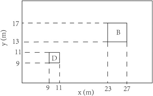22) )), with a self-adaptive method of successive averages (MSA) to handle the fixed-point problem (Du et al. 2013; Yang et al. 2022). A numerical example is given to demonstrate the proposed HB model. As shown in Figure 1, a 35 m long and 25 m wide rectangular modelling region is considered in the numerical experiment, and the centre of the destination is located at (10 m, 10 m) with a diameter of 2 m. A square obstacle where pedestrians are not allowed to enter or leave is located at (25 m, 15 m) with a diameter of 4 m. Set $T=100\mathrm{s}$; thus, the modelling period is $[0,100\mathrm{s}]$. We assume that there is no pedestrian at the beginning of the modelling period, i.e. ${\rho }_0(\mathit{x})=0,\mathrm{\forall }\mathit{x}\in \mathrm{\Omega }$. The penalty for a pedestrian not arriving at the destination on time is solved by (52) $\{\begin{array}{ll}\Vert \mathrm{\nabla }{\varphi }_0(\mathit{x})\Vert =\sqrt{2c_3(1+c_{2}r(d(\mathit{x},B)))},& \mathrm{\forall }\mathit{x}\in \mathrm{\Omega }\\ {\varphi }_0(\mathit{x})={\varphi }_D,& \mathrm{\forall }\mathit{x}\in {\mathrm{\Gamma }}_d\end{array}$(52) where $\mathit{x}=(x_1,x_2)$ and there is no cost to enter the destination; thus, ${\varphi }_D=0$. The travel demand function $q(\mathit{x},t)$ is defined as (53) $q(\mathit{x},t)=q_{max}[1-{\gamma }_1\mathrm{d}(\mathit{x})]\mathrm{d}(t)$(53) where $q_{max}=0.05\mathrm{ped}/({\mathrm{m}}^2\cdot \mathrm{s})$ is the maximum demand, $\mathrm{d}(\mathit{x})=\sqrt{(x_1-10{)}^2+(x_2-10{)}^2}$ is the distance from the location $\mathit{x}$ to the centre of the destination D, and ${\gamma }_1=0.01$. The factor $[1-{\gamma }_{1}d(\mathit{x})]$ represents the higher travel demand generated in the region closer to the destination, where more pedestrians live. $\mathrm{d}(t)$ is a non-negative function of the time variable t, and is defined as (54) $\mathrm{d}(t)=\{\begin{array}{ll}{\displaystyle \frac{t}{5},}& t\in [0,5\mathrm{s}]\\ {\displaystyle \frac{10-t}{5},}& t\in [5,10\mathrm{s}]\\ 0,& \mathrm{otherwise}\end{array}$(54)

Figure 1. The modelling domain.

For the local maximum admissible speed $V_0$ in Equation (3(3) $V_0=V_{max}\exp (-(\rho /{\rho }_e{)}^2)$(3) ), we take $V_{max}=1\mathrm{m}/\mathrm{s}$ (Xie and Wong 2015) and ${\rho }_e=2{\mathrm{ped}/\mathrm{m}}^2$. In the running cost L, the weights take values of $c_1=1,c_2=10,c_3=3$, and $c_4=1$ (Hoogendoorn and Bovy 2004a, 2004b). The cost around the obstacle $r(d(\mathit{x},B))$ is defined as (55) $r(\mathrm{d}(\mathit{x},B))=a\exp (-\frac{\mathrm{d}(\mathit{x},B)}{b})$(55) where a = 1 and b = 0.1 are the parameters. The part of the cost that depends on the density is defined as $\zeta (\rho )=0.3{\rho }^2$. We next show the numerical results obtained with a uniform mesh of $140\times 100$ grid points.

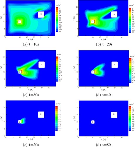
Figure 2 shows the spatial distribution of the density of pedestrian at different time. Pedestrians depart from their location and go to the destination within $[0,10\mathrm{s}]$. Thus, the northeast region of the destination boundary became congested (see sub-Figure 2(a,b)). Although the demand becomes zero from $t=10$ s, the areas around the destination are still in the congested condition at t = 30 s and t = 40 s due to the limitation on the maximum flow intensity into the destination (Sub-Figure 2(c,d). With the pedestrian entered the destination gradually, all parts of the region return to the non-congested condition eventually (Sub-Figure 2(e,f)).

Figure 2. density plot. (a) $t=10\mathrm{s}$. (b) $t=20\mathrm{s}$. (c) $t=30\mathrm{s}$. (d) $t=40\mathrm{s}$. (c) $t=50\mathrm{s}$. (d) $t=80\mathrm{s}$.

Figures 3 and 4 show the spatial distribution of the pedestrian speed $V^{\ast }$ and local maximum admissible speed $V_0$ at different times, respectively. The pedestrians walk faster when they are close to the destination or obstacle. As all of the pedestrians walk to the destination, the region around the destination (especially the northeast region) has a higher density; thus, the local maximum speed is small (Figure 4). According to the expression of $V_0$, when the density is zero, the local maximum speed is $V_0=1\mathrm{m}/\mathrm{s}$. However, a comparison of Figures 3 and 4 shows that the pedestrian speed $V^{\ast }$ is less than $V_0$ in the zero-density region. This is because the pedestrian speed also depends on travel time, energy consumption, distance to the obstacle, and pedestrian density. This is a peculiar property of the HB model.

Figure 3. Speed plot. (a) $t=10\mathrm{s}$. (b) $t=20\mathrm{s}$. (c) $t=30\mathrm{s}$. (d) $t=40\mathrm{s}$. (c) $t=50\mathrm{s}$. (d) $t=80\mathrm{s}$.

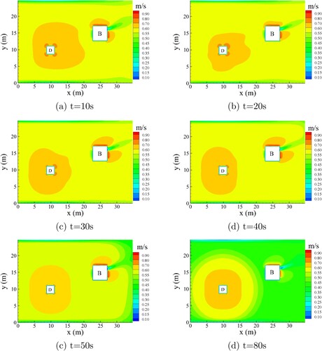
Figure 4. Maximum speed plot. (a) $t=10\mathrm{s}$. (b) $t=20\mathrm{s}$. (c) $t=30\mathrm{s}$. (d) $t=40\mathrm{s}$. (c) $t=50\mathrm{s}$. (d) $t=80\mathrm{s}$.

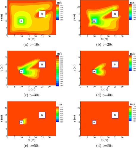
We define $k(\mathit{x},t)=V^{\ast }(\mathit{x},t)/V_0(\mathit{x},t)$ as the ratio of the pedestrian speed $V^{\ast }$ and local maximum admissible speed $V_0$. Figure 5 shows the spatial distribution of the ratio $k(\mathit{x},t)$ at different times. Figure 5 shows that the ratio is always less than 1, i.e. $V^{\ast }$ is always less than $V_0$. We also verified in the code that this is true for all locations and times. This demonstrates our conclusion of Theorem 2.1, namely, for weight parameters ($c_1,c_2,c_3,c_4$) satisfying certain conditions, $c_3^{-1}\Vert \mathrm{\nabla }\varphi \Vert \le V_0$ is always satisfied and the MASC is non-binding.

Figure 5. The plot of ratio of speed $V^{\ast }$ and local maximum admissible speed $V_0$. (a) $t=10\mathrm{s}$. (b) $t=20\mathrm{s}$. (c) $t=30\mathrm{s}$. (d) $t=40\mathrm{s}$. (c) $t=50\mathrm{s}$. (d) $t=80\mathrm{s}$.

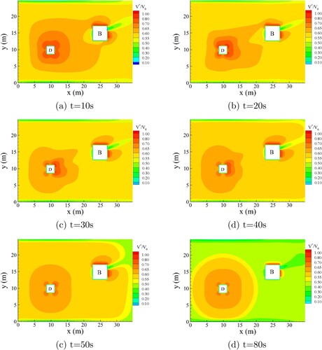
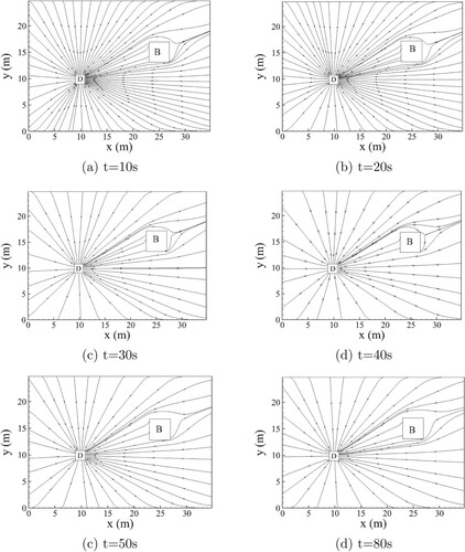
Figure 6 shows a plot of the velocity vector that reveals the pedestrian path choice. Pedestrians are observed to pass around the obstacle if they come from the east. In this example, the density is low; hence, pedestrians walk to the destination in nearly straight lines.

Figure 6. Velocity vector plot. (a) $t=10\mathrm{s}$. (b) $t=20\mathrm{s}$. (c) $t=30\mathrm{s}$. (d) $t=40\mathrm{s}$. (c) $t=50\mathrm{s}$. (d) $t=80\mathrm{s}$.

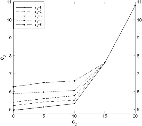
In fact, the original HB model is valid for all $c_3>0$, but we cannot prove this general case. From Theorem 2.1, we find that we can ignore the MASC in the Hamilton–Jacobi equation when $c_3\ge C(1+T)/V_{max}\exp (-(\theta /{\rho }_e{)}^2)$, where C depends on the values of $c_1,c_2$,and $c_4$, and thus the choices of values for $c_2$, $c_3$, and $c_4$ (assuming $c_1=1$) are closely related. If the values of $c_1,c_2$,and $c_4$ are known, we can use a value for $c_3$ that enables the MASC to be ignored (according to Theorem 2.1), and thus we define (56) $c_3^{\ast }=min\{c_3:c_3\ge \frac{C(1+T)}{V_{max}\exp (-(\theta /{\rho }_e{)}^2)}\}$(56) When $c_3<c_3^{\ast }$, this also represents the weighting of the cost associated with energy consumption, which is valid for the original HB model. However, we cannot ignore the MASC, i.e. there exists a location$x_0\in \mathrm{\Omega }$ and time $t_0$ such that $c_3^{-1}||\mathrm{\nabla }\varphi ({\mathit{x}}_0,t_0)||>V_0({\mathit{x}}_0,t_0)$, and thus we cannot prove the existence and uniqueness of the solution. In contrast, when $c_3\ge c_3^{\ast }$, we can ignore the MASC, i.e. $c_3^{-1}||\mathrm{\nabla }\varphi (\mathit{x},t)||\le V_0(\mathit{x},t)$ always holds. In Figure 7, we plot the value of $c_3^{\ast }$ versus $c_2$ for different $c_4$. We can observe that $c_3^{\ast }$ is an increasing function of both $c_2$ and $c_4$, and increases more rapidly for larger values of either $c_2$ or $c_4$. Furthermore, when $c_2$ takes a large value ($\ge$ 15), $c_3^{\ast }$ depends only on $c_2$ and is insensitive to a change in $c_4$.

Figure 7. The value of critical value $c_3^{\ast }$ with different $c_2$ and $c_4$.

5. Conclusions

In this study, we first briefly introduce the HB pedestrian-flow model (Hoogendoorn and Bovy 2004b), which describes pedestrian movements in continuous space and time. This model consists of a forward CL equation and backward HJB equation, in which the latter contains an MASC. It is difficult to prove the existence and uniqueness of the solution to this coupled model system with this MASC. Based on an analysis of the HB model, we find that if weight parameters satisfying certain conditions for use in the running cost function, the travel speed will always be less than the maximum admissible speed, and thus the MASC can be removed from the HB model. In this case, the HB model also contains a forward CL equation and a backward HJ equation, but lacks an MASC; hence, the analysis and computation of the HB model are simpler.

In Section 3, we consider the existence and uniqueness of the solution to the HB model. We first confirm the existence and uniqueness of the solution to the CL and HJ equations, and present some properties of the solutions to each. We then use the Schauder fixed-point theorem to show that the coupled HB model has a unique solution under certain assumptions. We use Lax-Friedrichs schemes for the CL and HJ equations, and use the self-adaptive MSA in the fixed-point problem to solve the HB model and provide a numerical example. This demonstrates that the travel speed is always less than the local maximum admissible speed if weight parameters satisfying certain conditions, which justifies the exclusion of the MASC in the analysis. We also explore the dependency of the model parameter $c_3$ (the weight for the energy consumption) as a function of the other two model parameters $c_2$ (the weight for the discomfort due to closeness to the obstacles) and $c_4$ (the weight for the part of the running cost that depends on the density) when the removal of the MASC is justified. The results show that $c_3$ is an increasing function of both $c_2$ and $c_4$. However, $c_3$ changes very little with changes in $c_4$, and can be approximately considered as a function only of $c_2$.

In this study, we only consider the existence and uniqueness of the solution to an HB model without an MASC. Although this is theoretically justified by the use of suitable model parameters and verified a posteriori by a numerical example with physical parameters chosen from the literature, there is no guarantee that the chosen physical parameters will ensure the exclusion of an MASC under all situations. Next, we will use the HB model to simulate the real-life pedestrian flow based on our analysis, and in turn, use the empirical results to calibrate the HB model. The existence and uniqueness of the solution to the HB model with an MASC (Hoogendoorn and Bovy 2004b) and the PDUO model (Du et al. 2013; Yang et al. 2022) are more difficult to analyse, because these models consist of coupled partial differential equations (the CL and HJ equations), a forward-backward structure, and are further complicated by the presence of an MASC. We will investigate these problems in our future work.

Disclosure statement

No potential conflict of interest was reported by the authors.

Additional information

Funding

The second author is supported by National Science Foundation (NSF) [grant number DMS-2010107] and AFOSR [grant number FA9550-20-1-0055]. The third author is supported by grants from the Research Grants Council of the Hong Kong Special Administrative Region, China [project numbers 17201318, 17204919), Guangdong - Hong Kong - Macau Joint Laboratory Program of the 2020 Guangdong New Innovative Strategic Research Fund, Guangdong Science and Technology Department [project number 2020B1212030009] and University of Hong Kong [Francis S Y Bong Professorship in Engineering] The fourth author is supported by National Natural Science Foundation of China (NSFC) [grant number 11871448].

Appendices

Appendix 1.

Proof of Theorem 3.4

Proof.

By the dynamic programming principle, Equation (24(24) $\{\begin{array}{ll}{\displaystyle -{\varphi }_t(\mathit{x},t)+\frac{1}{2c_3}|\mathrm{\nabla }\varphi {|}^2=g(\mathit{x},t),}& \mathrm{\forall }\mathit{x}\in \mathrm{\Omega },\mathrm{\forall }t\in [0,T]\\ \varphi (\mathit{x},t)={\varphi }_D(t),& \mathrm{\forall }\mathit{x}\in {\mathrm{\Gamma }}_d,\mathrm{\forall }t\in [0,T]\\ \varphi (\mathit{x},T)={\varphi }_0(\mathit{x}),& \mathrm{\forall }\mathit{x}\in \mathrm{\Omega }\end{array}$(24) ) has a bounded uniformly continuous viscosity solution, which can be written as $\varphi (\mathit{x},t)=\underset{\mathit{\alpha }\in L^2([t,T],R^2)}{inf}{\int }_t^T\frac{c_3}{2}|\mathit{\alpha }(s){|}^2+g(\mathit{x}(s),s)\mathrm{d}s+{\varphi }_0(\mathit{x}(T))$According to the dynamic programming principle, Hamiltonian in Equation (24(24) $\{\begin{array}{ll}{\displaystyle -{\varphi }_t(\mathit{x},t)+\frac{1}{2c_3}|\mathrm{\nabla }\varphi {|}^2=g(\mathit{x},t),}& \mathrm{\forall }\mathit{x}\in \mathrm{\Omega },\mathrm{\forall }t\in [0,T]\\ \varphi (\mathit{x},t)={\varphi }_D(t),& \mathrm{\forall }\mathit{x}\in {\mathrm{\Gamma }}_d,\mathrm{\forall }t\in [0,T]\\ \varphi (\mathit{x},T)={\varphi }_0(\mathit{x}),& \mathrm{\forall }\mathit{x}\in \mathrm{\Omega }\end{array}$(24) ) can be written as (A1) $H(\mathit{x},t,\mathit{p}):=\underset{\mathit{\alpha }\in L^2([t,T],R^2)}{min}\{\mathit{\alpha }\cdot \mathit{p}+\frac{c_3}{2}{\mathit{\alpha }}^2-g(\mathit{x},t)\}$(A1) Thus, $H(\mathit{x},t,\mathit{p})$ satisfies the conditions in Equation (27(27) $\{\begin{array}{ll}|H(\mathit{x},t,\mathit{p})-H(\mathit{x},t,\mathit{q})|\le C|\mathit{p}-\mathit{q}|,& \mathrm{\forall }\mathit{x}\in \mathrm{\Omega },\mathit{p},\mathit{q}\in R^2,\mathrm{\forall }t\in [0,T]\\ |H(\mathit{x},t,\mathit{p})-H(\mathit{y},t,\mathit{p})|\le C|\mathit{x}-\mathit{y}|(1+|\mathit{p}|),& \mathrm{\forall }\mathit{x},\mathit{y}\in \mathrm{\Omega },\mathit{p}\in R^2,\mathrm{\forall }t\in [0,T]\end{array}$(27) ), and $\varphi (\mathit{x},t)$ is the unique viscosity solution to Equation (24(24) $\{\begin{array}{ll}{\displaystyle -{\varphi }_t(\mathit{x},t)+\frac{1}{2c_3}|\mathrm{\nabla }\varphi {|}^2=g(\mathit{x},t),}& \mathrm{\forall }\mathit{x}\in \mathrm{\Omega },\mathrm{\forall }t\in [0,T]\\ \varphi (\mathit{x},t)={\varphi }_D(t),& \mathrm{\forall }\mathit{x}\in {\mathrm{\Gamma }}_d,\mathrm{\forall }t\in [0,T]\\ \varphi (\mathit{x},T)={\varphi }_0(\mathit{x}),& \mathrm{\forall }\mathit{x}\in \mathrm{\Omega }\end{array}$(24) ). We next check that the solution ϕ is Lipschitz with respect to variables $\mathit{x}$ and t. Let ${\mathit{x}}_1,{\mathit{x}}_2\in \mathrm{\Omega },t\in [0,T]$, $\mathit{\alpha }\in L^2([t,T],R^2)$ be ϵ-optimal for $\varphi ({\mathit{x}}_1,t)$, and set $\mathit{x}(s)={\mathit{x}}_1+{\int }_t^T\mathit{\alpha }(s)\mathrm{d}s$. Thus, we obtain (A2) ${\int }_t^T\frac{c_3}{2}|\mathit{\alpha }(s){|}^2+g(\mathit{x}(s),s)\mathrm{d}s+{\varphi }_0(\mathit{x}(T))\le \varphi ({\mathit{x}}_1,t)+ϵ$(A2) From the expression of $\varphi (\mathit{x},t)$ (Equation (30(30) $\varphi (\mathit{x},t)=\underset{\mathit{\alpha }\in L^2([t,T],R^2)}{inf}{\int }_t^T\frac{c_3}{2}|\mathit{\alpha }(s){|}^2+g(\mathit{x}(s),s)\mathrm{d}s+{\varphi }_0(\mathit{x}(T))$(30) )), we have (A3) $\begin{array}{rl}\varphi ({\mathit{x}}_2,t)& \le {\int }_t^T\frac{c_3}{2}|\mathit{\alpha }(s){|}^2+g(\mathit{x}(s)+{\mathit{x}}_2-{\mathit{x}}_1,s)\mathrm{d}s+{\varphi }_0(\mathit{x}(T)+{\mathit{x}}_2-{\mathit{x}}_1)\\ & \le {\int }_t^T\frac{c_3}{2}|\mathit{\alpha }(s){|}^2+(g(\mathit{x}(s),s)+C|{\mathit{x}}_2-{\mathit{x}}_1|)\mathrm{d}s+{\varphi }_0(\mathit{x}(T))+C|{\mathit{x}}_2-{\mathit{x}}_1|\\ & \le {\int }_t^T\frac{c_3}{2}|\mathit{\alpha }(s){|}^2+g(\mathit{x}(s),s)\mathrm{d}s+{\varphi }_0(\mathit{x}(T))+C(1+T)|{\mathit{x}}_2-{\mathit{x}}_1|\\ & \le \varphi ({\mathit{x}}_1,t)+ϵ+C(1+T)|{\mathit{x}}_1-{\mathit{x}}_2|\end{array}$(A3) Thus, ϕ is Lipschitz continuous with respect to the variable $\mathit{x}$, and the Lipschitz constant is $C(1+T)$.

From the dynamic programming principle, if $\mathit{\alpha }$ is optimal for $\varphi (\mathit{x},t)$ in Equation (30(30) $\varphi (\mathit{x},t)=\underset{\mathit{\alpha }\in L^2([t,T],R^2)}{inf}{\int }_t^T\frac{c_3}{2}|\mathit{\alpha }(s){|}^2+g(\mathit{x}(s),s)\mathrm{d}s+{\varphi }_0(\mathit{x}(T))$(30) ), from the equivalent definition of the dynamic programming principle for any $t<s\le T$, we have (A4) $\varphi (\mathit{x},t)={\int }_t^s\frac{c_3}{2}|\mathit{\alpha }(\tau ){|}^2+g(\mathit{x}(\tau ),\tau )\mathrm{d}\tau +\varphi (\mathit{x}(s),s)$(A4) Now let $\mathit{x}\in \mathrm{\Omega }$, $0\le t<\hat{t}\le T$. Take $ϵ>0$ and choose $\mathit{\alpha }$ to satisfy (A5) $\varphi (\mathit{x},t)+ϵ\ge {\int }_t^T\frac{c_3}{2}|\mathit{\alpha }(s){|}^2+g(\mathit{x}(s),s)\mathrm{d}s+{\varphi }_0(\mathit{x}(T))$(A5) where $\mathit{x}(s)=\mathit{x}+{\int }_t^s\mathit{\alpha }(\tau )\mathrm{d}\tau$. Define (A6) $\hat{\mathit{\alpha }}(s):=\mathit{\alpha }(s+t-\hat{t})\mathrm{for}\hat{t}\le s\le T$(A6) We can then define the related $\hat{\mathit{x}}(s)$ as (A7) $\hat{\mathit{x}}(s)=\mathit{x}+{\int }_t^s\hat{\mathit{\alpha }}(\tau )\mathrm{d}\tau =\mathit{x}(s+t-\hat{t})$(A7) Hence (A8) $\begin{array}{rl}\varphi (\mathit{x},\hat{t})-\varphi (\mathit{x},t)& \le {\int }_{\hat{t}}^T\frac{c_3}{2}|\hat{\mathit{\alpha }}(s){|}^2+g(\hat{\mathit{x}}(s),s)\mathrm{d}s+{\varphi }_0(\hat{\mathit{x}}(T))\\ & -{\int }_t^T\frac{c_3}{2}|\mathit{\alpha }(s){|}^2+{\varphi }_0(\mathit{x}(s),s)\mathrm{d}s-{\varphi }_0(\mathit{x}(T))+ϵ\\ & =-{\int }_{T-t-\hat{t}}^T\frac{c_3}{2}|\mathit{\alpha }(s){|}^2+g(\mathit{x}(s),s)\mathrm{d}s+{\varphi }_0(\mathit{x}(T+t-\hat{t}))-{\varphi }_0(\mathit{x}(T))+ϵ\\ & \le {\int }_{T-t-\hat{t}}^T(\frac{c_3}{2}\Vert \mathit{\alpha }{\Vert }_{\mathrm{\infty }}+\Vert g(\cdot ,s){\Vert }_{\mathrm{\infty }})\mathrm{d}s+{\varphi }_0(\mathit{x}(T+t-\hat{t}))-{\varphi }_0(\mathit{x}(T))+ϵ\\ & \le C|t-\hat{t}|+ϵ\end{array}$(A8) Additionally, we can take $\hat{\mathit{\alpha }}$ satisfying (A9) $\varphi (\mathit{x},\hat{t})+ϵ\ge {\int }_{\hat{t}}^T\frac{c_3}{2}|\hat{\mathit{\alpha }}(s){|}^2+g(\hat{\mathit{x}}(s),s)\mathrm{d}s+{\varphi }_0(\hat{\mathit{x}}(T))$(A9) where $\hat{\mathit{x}}(s)=\mathit{x}+{\int }_{\hat{t}}^s\hat{\mathit{\alpha }}(\tau )\mathrm{d}\tau$, then, we define (A10) $\mathit{\alpha }(s)=\{\begin{array}{ll}\hat{\mathit{\alpha }}(s+\hat{t}-t)& \mathrm{if}t\le s\le T+t-\hat{t}\\ \hat{\mathit{\alpha }}(T)& \mathrm{if}T+t-\hat{t}\le s\le T\end{array}$(A10) Similarly, we can define the related $\mathit{x}(s)=\mathit{x}+{\int }_t^T\mathit{\alpha }(\tau )\mathrm{d}\tau$, and thus, $\mathit{\alpha }(s)=\hat{\mathit{\alpha }}(s+\hat{t}-t)$ $\mathit{x}(s)=\hat{\mathit{x}}(s+\hat{t}-t)$ for $t\le s\le T+t-\hat{t}$. Then (A11) $\begin{array}{rl}\varphi (\mathit{x},t)-\varphi (\mathit{x},\hat{t})& \le {\int }_t^T\frac{c_3}{2}|\mathit{\alpha }(s){|}^2+g(\mathit{x}(s),s)\mathrm{d}s+{\varphi }_0(\mathit{x}(T))\\ & -{\int }_{\hat{t}}^T\frac{c_3}{2}|\hat{\mathit{\alpha }}(s){|}^2+g(\hat{\mathit{x}}(s),s)\mathrm{d}s-{\varphi }_0(\hat{\mathit{x}}(T))+ϵ\\ & ={\int }_{T+t-\hat{t}}^T\frac{c_3}{2}|\mathit{\alpha }(s){|}^2+g(\mathit{x}(s),s)\mathrm{d}s-{\varphi }_0(\mathit{x}(T+t-\hat{t}))+{\varphi }_0(\mathit{x}(T))+ϵ\\ & ={\int }_{T+t-\hat{t}}^T\frac{1}{2}(\frac{c_3}{2}\Vert \mathit{\alpha }{\Vert }_{\mathrm{\infty }}+\Vert g(\cdot ,s){\Vert }_{\mathrm{\infty }})\mathrm{d}s-{\varphi }_0(\mathit{x}(T+t-\hat{t}))+{\varphi }_0(\mathit{x}(T))+ϵ\\ & \le C|t-\hat{t}|+ϵ\end{array}$(A11) Consequently, we have (A12) $|\varphi (\mathit{x},t)-\varphi (\mathit{x},\hat{t})|\le C|t-\hat{t}|$(A12) Next, we show that ϕ is semi-concave with respect to the variable $\mathit{x}$. Let $\mathit{x},\mathit{y}\in \mathrm{\Omega }$, $t\in [0,T]$, $\lambda \in (0,1)$ and ${\mathit{x}}_{\lambda }=\lambda \mathit{x}+(1-\lambda )\mathit{y}$. Let also $\mathit{\alpha }\in L^2([t,T],R^2)$ be ϵ-optimal for $\varphi ({\mathit{x}}_{\lambda },t)$, and set ${\mathit{x}}_{\lambda }(s)={\mathit{x}}_{\lambda }+{\int }_t^s\mathit{\alpha }(\tau )\mathrm{d}\tau$. Then (A13) $\begin{array}{rl}& \lambda \varphi (\mathit{x},t)+(1-\lambda )\varphi (\mathit{y},t)\\ & \le \lambda {\int }_t^T\frac{c_3}{2}|\mathit{\alpha }(s){|}^2+g({\mathit{x}}_{\lambda }(s)+\mathit{x}-{\mathit{x}}_{\lambda },s)\mathrm{d}s+{\varphi }_0({\mathit{x}}_{\lambda }(T)+\mathit{x}-{\mathit{x}}_{\lambda })\\ & +(1-\lambda ){\int }_t^T\frac{c_3}{2}|\mathit{\alpha }(s){|}^2+g({\mathit{x}}_{\lambda }(s)+\mathit{y}-{\mathit{x}}_{\lambda },s)\mathrm{d}s+{\varphi }_0({\mathit{x}}_{\lambda }(T)+\mathit{y}-{\mathit{x}}_{\lambda })\\ & \le {\int }_t^T\frac{c_3}{2}|\mathit{\alpha }(s){|}^2+g({\mathit{x}}_{\lambda }(s),s)\mathrm{d}s+{\varphi }_0({\mathit{x}}_{\lambda }(T))+C(1+T)\lambda (1-\lambda )|\mathit{x}-\mathit{y}{|}^2\\ & \le \varphi ({\mathit{x}}_{\lambda },t)+ϵ+C(1+T)\lambda (1-\lambda )|\mathit{x}-\mathit{y}{|}^2\end{array}$(A13) Thus, from Definition 3.3, ϕ is semi-concave, and the semi-concavity constant is $C(1+T)$.

Appendix 2.

Proof of Theorem 3.8

Proof.

To prove this theorem, we only need to show that the coefficients $A_1$ and $A_2$ satisfy the conditions (33(33) $|A_i(\mathit{x},t)|\le C,\mathrm{\forall }\mathit{x}\in \mathrm{\Omega },i=1,2$(33) ) and (34(34) $⟨\mathit{A}(\mathit{x},t)-\mathit{A}(\mathit{y},t),\mathit{x}-\mathit{y}⟩\ge -m(t)|\mathit{x}-\mathit{y}{|}^2,\mathrm{\forall }\mathit{x},\mathit{y}\in \mathrm{\Omega }$(34) ). In our problem (A14) $\mathit{A}(\mathit{x},t)=-c_3^{-1}\mathrm{\nabla }\varphi (\mathit{x},t)$(A14) By the analysis for the HJ equation, we know that ϕ is Lipschitz continuous and semi-concave; thus, condition (33(33) $|A_i(\mathit{x},t)|\le C,\mathrm{\forall }\mathit{x}\in \mathrm{\Omega },i=1,2$(33) ) is satisfied. By the equivalent definition of semi-concavity, we have (A15) $⟨\mathit{p}-\mathit{q},\mathit{x}-\mathit{y}⟩\le C|\mathit{x}-\mathit{y}{|}^2$(A15) where C>0, $\mathit{p}\in D_{\mathit{x}}^{+}\varphi (\mathit{x},t)$, and $\mathit{q}\in D_{\mathit{x}}^{+}(\mathit{y},t)$ because $\mathrm{\nabla }\varphi (\mathit{x},t)\in D_{\mathit{x}}^{+}(\mathit{x},t)$. We then have (A16) $⟨\mathrm{\nabla }\varphi (\mathit{x},t)-\mathrm{\nabla }\varphi (\mathit{y},t),\mathit{x}-\mathit{y}⟩\le C|x-y{|}^2$(A16) Because $A(x,t)=-\mathrm{\nabla }\varphi (x,t)$, we obtain (A17) $⟨\mathit{A}(\mathit{x},t)-\mathit{A}(\mathit{y},t),\mathit{x}-\mathit{y}⟩\ge -C|\mathit{x}-\mathit{y}{|}^2$(A17) Thus, the one-sided Lipschitz condition holds for $m(t)=C$. According to Theorem 3.6, the conservation law (Equation (23(23) $\{\begin{array}{ll}{\rho }_t+\mathrm{\nabla }\cdot (-\rho c_3^{-1}\mathrm{\nabla }\varphi )=q(\mathit{x},t),& \mathrm{\forall }\mathit{x}\in \mathrm{\Omega },\mathrm{\forall }t\in [0,T]\\ \rho (\mathit{x},0)={\rho }_0(\mathit{x}),& \mathrm{\forall }\mathit{x}\in \mathrm{\Omega }\\ \rho (\mathit{x},t)=0.& \mathrm{\forall }\mathit{x}\in {\mathrm{\Gamma }}_i\cup {\mathrm{\Gamma }}_b,\mathrm{\forall }t\in [0,T]\end{array}$(23) )) has a unique weak solution so that the theorem holds.

Appendix 3.

Proof of Lemma 3.9

Proof.

From our assumptions regarding F and ${\varphi }_0$, the sequences of the map $(\mathit{x},t)\to F(\mathit{x},m_n)$ and $(x,t)\to {\varphi }_0(\mathit{x},m_n)$ locally uniformly converge to the map $(\mathit{x},t)\to F(\mathit{x},m)$ and $(x,t)\to {\varphi }_0(\mathit{x},m)$, respectively. Thus, by the stability of the viscosity solution (Lin and Tadmor 2001), $\{{\varphi }_n\}$ locally uniformly converges to ϕ.

According to Lemma 3.5, ${\varphi }_n$ is semi-concave, i.e. there exists a constant $C_1$ such that $D_{\mathit{x}\mathit{x}}^2{\varphi }_n\le C_1{I}_d$ for all n. Because the solutions ${\varphi }_n$ locally uniformly converge to ϕ, $D_{\mathit{x}}{\varphi }_n$ converges almost everywhere in $\mathrm{\Omega }\times (0,T)$ to $D_{\mathit{x}}\varphi$ (Cannarsa and Sinestrari 2004). From the consideration of the conservation law equation, ${\rho }_n\in C([0,T],{\mathcal{P}}_1)$ and Ω is a bounded closed domain. There then exists a constant C independent of n such that (A18) ${\mathit{d}}_1({\rho }_n(t)-{\rho }_n(s))\le C|t-s|,\mathrm{\forall }t,s\in [0,T],\mathrm{\forall }n>0$(A18) From the above inequality, ${\rho }_n$ is equi-continuous. Additionally, ${\rho }_n$ is clearly uniformly bounded in $\mathrm{\Omega }\times [0,T]$ and the set ${\mathcal{P}}_1$ is compact. Hence by the Arzel$\stackrel{`}{\mathrm{a}}$-Ascoli theorem, the sequence $\{{\rho }_n\}$ has a subsequence (still denoted as $\{{\rho }_n\}$) that converges in $\mathcal{C}$, with the limit denoted as ${\rho }^{\ast }$. Because ${\rho }_n$ solves the continuity equation for ${\varphi }_n$, one easily passes the limit such that ${\rho }^{\ast }$ satisfies the continuity equation for ϕ by the uniqueness that implies ${\rho }^{\ast }=\rho$; thus, the proof is complete.

Appendix 4.

Proof of Theorem 3.10

Proof.

Assume $({\varphi }_1,{\rho }_1)$ and $({\varphi }_2,{\rho }_2)$ are two pairs of solutions to the problem. We set $\overline{\varphi }={\varphi }_1-{\varphi }_2$ and $\overline{\rho }={\rho }_1-{\rho }_2$. Then (A19) $\begin{array}{rl}-\frac{\mathrm{\partial }\overline{\varphi }}{\mathrm{\partial }t}+\frac{1}{2c_3}|\mathrm{\nabla }{\varphi }_1{|}^2-\frac{1}{2c_3}|\mathrm{\nabla }{\varphi }_2{|}^2& =F(\mathit{x},{\rho }_1)-\varphi (\mathit{x},{\rho }_2)\end{array}$(A19) (A20) $\begin{array}{rl}\frac{\mathrm{\partial }\overline{\rho }}{\mathrm{\partial }t}+c_3^{-1}\mathrm{\nabla }\cdot (-{\rho }_1\mathrm{\nabla }{\varphi }_1+{\rho }_2\mathrm{\nabla }{\varphi }_2)& =0\end{array}$(A20) Next, let us use $\overline{\varphi }$ as a test function in the second equation (we may need to regularize and truncate $\overline{\varphi }$ to $C_c^1(\mathrm{\Omega }\times [0,T))$, after which we still denote it as $\overline{\varphi }$). We then have (A21) $\begin{array}{rl}& -{\int }_{\mathrm{\Omega }}(\overline{\rho }\overline{\varphi })(T)\mathrm{d}\mathit{x}+{\int }_{\mathrm{\Omega }}(\overline{\rho }\overline{\varphi })(0)\mathrm{d}\mathit{x}+{\int }_{\mathrm{\Omega }}{\int }_0^T\frac{\mathrm{\partial }\overline{\varphi }}{\mathrm{\partial }t}\overline{\rho }\mathrm{d}t\mathrm{d}\mathit{x}\\ & +{\int }_{\mathrm{\Omega }}{\int }_0^T{c}_3^{-1}⟨\mathrm{\nabla }\overline{\varphi },{\rho }_1\mathrm{\nabla }{\varphi }_1-{\rho }_2\mathrm{\nabla }{\varphi }_2⟩\mathrm{d}t\mathrm{d}\mathit{x}=0\end{array}$(A21) Let us multiply Equation (A19(A19) $\begin{array}{rl}-\frac{\mathrm{\partial }\overline{\varphi }}{\mathrm{\partial }t}+\frac{1}{2c_3}|\mathrm{\nabla }{\varphi }_1{|}^2-\frac{1}{2c_3}|\mathrm{\nabla }{\varphi }_2{|}^2& =F(\mathit{x},{\rho }_1)-\varphi (\mathit{x},{\rho }_2)\end{array}$(A19) ) by $\overline{\rho }$, integrate over $\mathrm{\Omega }\times (0,T)$, and add the result to the previous equality. After simplification and using $\overline{\rho }(\mathit{x},0)=0$, we obtain (A22) $\begin{array}{rl}& -{\int }_{\mathrm{\Omega }}(\overline{\rho }\overline{\varphi })(T)\mathrm{d}\mathit{x}+{\int }_{\mathrm{\Omega }}{\int }_0^T\frac{1}{2c_3}\overline{\rho }(|\mathrm{\nabla }{\varphi }_1{|}^2-|\mathrm{\nabla }{\varphi }_2{|}^2)-\overline{\rho }(F(\mathit{x},{\varphi }_1)-F(\mathit{x},{\varphi }_2))\mathrm{d}t\mathrm{d}\mathit{x}\\ & -{\int }_{\mathrm{\Omega }}{\int }_0^T{c}_3^{-1}⟨\mathrm{\nabla }\overline{\varphi },{\rho }_1\mathrm{\nabla }{\varphi }_1-{\rho }_2\mathrm{\nabla }{\varphi }_2⟩\mathrm{d}t\mathrm{d}\mathit{x}=0\end{array}$(A22) Note that (A23) $\begin{array}{rl}& \frac{1}{2c_3}\overline{\rho }(|\mathrm{\nabla }{\varphi }_1{|}^2-|\mathrm{\nabla }{\varphi }_2{|}^2)-c_3^{-1}⟨\mathrm{\nabla }\overline{\varphi },{\rho }_1\mathrm{\nabla }{\varphi }_1-{\rho }_2\mathrm{\nabla }{\varphi }_2⟩\\ & =-c_3^{-1}[\frac{1}{2}{\rho }_1|\mathrm{\nabla }{\varphi }_1{|}^2+\frac{1}{2}{\rho }_2|\mathrm{\nabla }{\varphi }_2{|}^2+\frac{1}{2}{\rho }_1|\mathrm{\nabla }{\varphi }_2{|}^2+\frac{1}{2}{\rho }_2|\mathrm{\nabla }{\varphi }_1{|}^2-({\rho }_1+{\rho }_2)\mathrm{\nabla }{\varphi }_1\cdot \mathrm{\nabla }{\varphi }_2]\\ & =-\frac{1}{2c_3}[({\rho }_1+{\rho }_2)(|\mathrm{\nabla }{\varphi }_1{|}^2+|\mathrm{\nabla }{\varphi }_2{|}^2)-2({\rho }_1+{\rho }_2)\mathrm{\nabla }{\varphi }_1\cdot \mathrm{\nabla }{\varphi }_2]\\ & =-\frac{1}{2c_3}[({\rho }_1+{\rho }_2)|\mathrm{\nabla }{\varphi }_1-\mathrm{\nabla }{\varphi }_2{|}^2]\\ & \le 0\end{array}$(A23) and (A24) ${\int }_{\mathrm{\Omega }}\overline{\rho }\overline{\varphi }(T)\mathrm{d}\mathit{x}={\int }_{\mathrm{\Omega }}({\rho }_1-{\rho }_2)(T)({\varphi }_{1,0}(\mathit{x},{\rho }_1)-{\varphi }_{2,0}(\mathit{x},{\rho }_2))\mathrm{d}\mathit{x}\ge 0$(A24) Because $F(\mathit{x},\rho )=c_1+c_{2}r(d(\mathit{x},B))+c_4\zeta (\rho (\mathit{x},t))$, where $c_4>0$ and ζ is strictly monotonically increasing about ρ, we have (A25) $({\rho }_1-{\rho }_2)(F(\mathit{x},{\rho }_1)-F(\mathit{x},{\rho }_2))>0,\mathrm{if}{\rho }_1\ne {\rho }_2$(A25) Combining Equations (A23(A23) $\begin{array}{rl}& \frac{1}{2c_3}\overline{\rho }(|\mathrm{\nabla }{\varphi }_1{|}^2-|\mathrm{\nabla }{\varphi }_2{|}^2)-c_3^{-1}⟨\mathrm{\nabla }\overline{\varphi },{\rho }_1\mathrm{\nabla }{\varphi }_1-{\rho }_2\mathrm{\nabla }{\varphi }_2⟩\\ & =-c_3^{-1}[\frac{1}{2}{\rho }_1|\mathrm{\nabla }{\varphi }_1{|}^2+\frac{1}{2}{\rho }_2|\mathrm{\nabla }{\varphi }_2{|}^2+\frac{1}{2}{\rho }_1|\mathrm{\nabla }{\varphi }_2{|}^2+\frac{1}{2}{\rho }_2|\mathrm{\nabla }{\varphi }_1{|}^2-({\rho }_1+{\rho }_2)\mathrm{\nabla }{\varphi }_1\cdot \mathrm{\nabla }{\varphi }_2]\\ & =-\frac{1}{2c_3}[({\rho }_1+{\rho }_2)(|\mathrm{\nabla }{\varphi }_1{|}^2+|\mathrm{\nabla }{\varphi }_2{|}^2)-2({\rho }_1+{\rho }_2)\mathrm{\nabla }{\varphi }_1\cdot \mathrm{\nabla }{\varphi }_2]\\ & =-\frac{1}{2c_3}[({\rho }_1+{\rho }_2)|\mathrm{\nabla }{\varphi }_1-\mathrm{\nabla }{\varphi }_2{|}^2]\\ & \le 0\end{array}$(A23) ), (A24(A24) ${\int }_{\mathrm{\Omega }}\overline{\rho }\overline{\varphi }(T)\mathrm{d}\mathit{x}={\int }_{\mathrm{\Omega }}({\rho }_1-{\rho }_2)(T)({\varphi }_{1,0}(\mathit{x},{\rho }_1)-{\varphi }_{2,0}(\mathit{x},{\rho }_2))\mathrm{d}\mathit{x}\ge 0$(A24) ), and (A25(A25) $({\rho }_1-{\rho }_2)(F(\mathit{x},{\rho }_1)-F(\mathit{x},{\rho }_2))>0,\mathrm{if}{\rho }_1\ne {\rho }_2$(A25) ) we obtain (A26) $\begin{array}{rl}& -{\int }_{\mathrm{\Omega }}(\overline{\rho }\overline{\varphi })(T)\mathrm{d}\mathit{x}+{\int }_{\mathrm{\Omega }}{\int }_0^T\frac{1}{2c_3}\overline{\rho }(|\mathrm{\nabla }{\varphi }_1{|}^2-|\mathrm{\nabla }{\varphi }_2{|}^2)-\overline{\rho }(F(\mathit{x},{\varphi }_1)-F(\mathit{x},{\varphi }_2))\mathrm{d}t\mathrm{d}\mathit{x}\\ & -{\int }_{\mathrm{\Omega }}{\int }_0^T{c}_3^{-1}⟨\mathrm{\nabla }\overline{\varphi },{\rho }_1\mathrm{\nabla }{\varphi }_1-{\rho }_2\mathrm{\nabla }{\varphi }_2⟩\mathrm{d}t\mathrm{d}\mathit{x}<0\mathrm{if}{\rho }_1\ne {\rho }_2\end{array}$(A26) This contradicts with Equation (A22(A22) $\begin{array}{rl}& -{\int }_{\mathrm{\Omega }}(\overline{\rho }\overline{\varphi })(T)\mathrm{d}\mathit{x}+{\int }_{\mathrm{\Omega }}{\int }_0^T\frac{1}{2c_3}\overline{\rho }(|\mathrm{\nabla }{\varphi }_1{|}^2-|\mathrm{\nabla }{\varphi }_2{|}^2)-\overline{\rho }(F(\mathit{x},{\varphi }_1)-F(\mathit{x},{\varphi }_2))\mathrm{d}t\mathrm{d}\mathit{x}\\ & -{\int }_{\mathrm{\Omega }}{\int }_0^T{c}_3^{-1}⟨\mathrm{\nabla }\overline{\varphi },{\rho }_1\mathrm{\nabla }{\varphi }_1-{\rho }_2\mathrm{\nabla }{\varphi }_2⟩\mathrm{d}t\mathrm{d}\mathit{x}=0\end{array}$(A22) ), so ${\rho }_1={\rho }_2$; therefore, ${\varphi }_1$ and ${\varphi }_2$ solve the same equation; thus, ${\varphi }_1={\varphi }_2$ and the uniqueness of the coupled model system holds.

References

- Aghamohammadi, R., and J. A. Laval. 2020. “Dynamic Traffic Assignment Using the Macroscopic Fundamental Diagram: A Review of Vehicular and Pedestrian Flow Models.” Transportation Research Part B: Methodological 137: 99–118.
- Asano, M., T. Iryo, and M. Kuwahara. 2010. “Microscopic Pedestrian Simulation Model Combined with a Tactical Model for Route Choice Behaviour.” Transportation Research Part C: Emerging Technologies18 (6): 842–855.
- Bouchut, F., and F. James. 1998. “One-Dimensional Transport Equations with Discontinuous Coefficients.” Nonlinear Analysis: Theory, Methods & Applications 32 (7): 891–933.
- Bressan, A., and K. Han. 2013. “Existence of Optima and Equilibria for Traffic Flow on Networks.” Networks and Heterogeneous Media 8 (3): 627–648.
- Cannarsa, P., and C. Sinestrari. 2004. 'Semiconcave Functions, Hamilton–Jacobi Equations, and Optimal Control. Vol. 58. Boston, MA: Springer Science & Business Media.
- Cardaliaguet, P. 2010. “Notes on Mean Field Games (p. 120).” Technical Report.
- Conway, E. D.. 1967. “Generalized Solutions of Linear Differential Equations with Discontinuous Coefficients and the Uniqueness Question for Multidimensional Quasilinear Conservation Laws.” Journal of Mathematical Analysis and Applications 18 (2): 238–251.
- Crandall, M. G., L. C. Evans, and P. L. Lions. 1984. “Some Properties of Viscosity Solutions of Hamilton–Jacobi Equations.” Transactions of the American Mathematical Society 282 (2): 487–502.
- Crandall, M. G., and P. L. Lions. 1983. “Viscosity Solutions of Hamilton–Jacobi Equations.” Transactions of the American Mathematical Society 277 (1): 1–42.
- Crociani, L., and G. Laemmel. 2016. “Multidestination Pedestrian Flows in Equilibrium: A Cellular Automaton-Based Approach.” Computer-Aided Civil and Infrastructure Engineering 31 (6): 432–448.
- Dolcetta, I. C., and B. Perthame. 1996. “On Some Analogy Between Different Approaches to First Order PDE's with Non Smooth Coefficients.” Advances in Mathematical Sciences and Applications 6: 689–703.
- Du, J., S. C. Wong, C. W. Shu, T. Xiong, M. P. Zhang, and K Choi. 2013. “Revisiting Jiang's Dynamic Continuum Model for Urban Cities.” Transportation Research Part B: Methodological 56: 96–119.
- Evans, L. C.. 1998. Partial Differential Equations. Providence, RI: American Mathematical Society.
- Fathi, A.. 2011. “On Existence of Smooth Critical Subsolutions of the Hamilton–Jacobi Equation.” Publicaciones Matemáticas del Uruguay 12: 87–98.
- Fleming, W. H.. 1969. “The Cauchy Problem for a Nonlinear First Order Partial Differential Equation.” Journal of Differential Equations 5 (3): 515–530.
- Fosgerau, M., E. Frejinger, and A. Karlstrom. 2013. “A Link Based Network Route Choice Model with Unrestricted Choice Set.” Transportation Research Part B: Methodological 56 (1): 70–80.
- Frejinger, E., M. Bierlaire, and M. Ben-Akiva. 2009. “Sampling of Alternatives for Route Choice Modeling.” Transportation Research Part B: Methodological 43 (10): 984–994.
- Friedman, A., and E. Hopf. 1973. “The Cauchy Problem for First Order Partial Differential Equations.” Indiana University Mathematics Journal 23 (1): 27–40.
- Gao, Z., Y. Qu, X. Li, J. Long, and H. J. Huang. 2014. “Simulating the Dynamic Escape Process in Large Public Places.” Operations Research 62 (6): 1344–1357.
- Han, K., T. L. Friesz, and T. Yao. 2013. “Existence of Simultaneous Route and Departure Choice Dynamic User Equilibrium.” Transportation Research Part B: Methodological 53: 17–30.
- Hoogendoorn, S. P., and P. H. Bovy. 2004a. “Pedestrian Route-Choice and Activity Scheduling Theory and Models.” Transportation Research Part B: Methodological 38 (2): 169–190.
- Hoogendoorn, S. P., and P. H. Bovy. 2004b. “Dynamic User-Optimal Assignment in Continuous Time and Space.” Transportation Research Part B: Methodological 38 (7): 571–592.
- Huang, L., S. C. Wong, M. Zhang, C. W. Shu, and W. H. Lam. 2009. “Revisiting Hughes' Dynamic Continuum Model for Pedestrian Flow and the Development of An Efficient Solution Algorithm.” Transportation Research Part B: Methodological 43 (1): 127–141.
- Hughes, R. L.. 2002. “A Continuum Theory for the Flow of Pedestrians.” Transportation Research Part B: Methodological 36 (6): 507–535.
- Lam, W. H., C. Y. Cheung, and C. F. Lam. 1999. “A Study of Crowding Effects At the Hong Kong Light Rail Transit Stations.” Transportation Research Part A: Policy and Practice 33 (5): 401–415.
- Lam, H. K. W., J. F. Morrall, and H. Ho. 1995. “Pedestrian Flow Characteristics in Hong Kong.” Transportation Research Record 1487: 56–62.
- Lasry, J. M., and P. L. Lions. 2007. “Mean Field Games.” Japanese Journal of Mathematics 2 (1): 229–260.
- Lax, P. D.. 1954. “Weak Solutions of Nonlinear Hyperbolic Equations and Their Numerical Computation.” Communications on Pure and Applied Mathematics 7 (1): 159–193.
- Lax, P. D.. 1971. “Shock Waves and Entropy.” In Contributions to Nonlinear Functional Analysis, 603–634. Academic Press.
- Lin, C. T., and E. Tadmor. 2001. “L1-Stability and Error Estimates for Approximate Hamilton–Jacobi Solutions.” Numerische Mathematik 87 (4): 701–735.
- Lin, Z., P. Zhang, and H. Hang. 2022. “A Dynamic Continuum Route Choice Model for Pedestrian Flow with Mixed Crowds.” Transportmetrica A: Transport Science 1–26. doi:10.1080/23249935.2022.2075951.
- Lions, P. L.. 1982. Generalized Solutions of Hamilton–Jacobi Equations. Vol. 69. London: Pitman.
- Mai, T., M. Fosgerau, and E. Frejinger. 2015. “A Nested Recursive Logit Model for Route Choice Analysis.” Transportation Research Part B: Methodological 75 (5): 100–112.
- Morrall, J. F., L. L. Ratnayake, and P. N. Seneviratne. 1991. “Comparison of Central Business District Pedestrian Characteristics in Canada and Sri Lanka.” Transportation Research Record 1294: 57–61.
- Petrova, G., and B. Popov. 1999. “Linear Transport Equations with Discontinuous Coefficients.” Communications in Partial Differential Equations 24 (9–10): 1849–1873.
- Plaue, M., M. Chen, G. B'arwolff, and H. Schwandt. 2011. “Trajectory Extraction and Density Analysis of Intersecting Pedestrian Flows from Video Recordings.” In ISPRS Conference on Photogrammetric Image Analysis, 285–296. Berlin, Heidelberg: Springer.
- Plaue, M., M. Chen, G. B'arwolff, and H. Schwandt. 2012. “Multi-View Extraction of Dynamic Pedestrian Density Fields.” Photogrammetrie-Fernerkundung-Geoinformation 2012 (5): 547–555.
- Sánchez-Morgado, H., P. Padilla, R. Iturriaga, and N. Anantharaman. 2012. “Physical Solutions of the Hamilton–Jacobi Equation.” Discrete and Continuous Dynamical Systems -- Series B 5 (3): 513–528.
- Tadmor, E.. 1991. “Local Error Estimates for Discontinuous Solutions of Nonlinear Hyperbolic Equations.” SIAM Journal on Numerical Analysis 28 (4): 891–906.
- Taherifar, N., H. Hamedmoghadam, S. Sree, and M. Saberi. 2019. “A Macroscopic Approach for Calibration and Validation of a Modified Social Force Model for Bidirectional Pedestrian Streams.” Transportmetrica A: Transport Science 15 (2): 1637–1661.
- Wong, S. C., W. L. Leung, S. H. Chan, W. H. Lam, N. H. Yung, C. Y. Liu, and P. Zhang. 2010. “Bidirectional Pedestrian Stream Model with Oblique Intersecting Angle.” Journal of Transportation Engineering 136 (3): 234–242.
- Xie, S., and S. C. Wong. 2015. “A Bayesian Inference Approach to the Development of a Multidirectional Pedestrian Stream Model.” Transportmetrica A: Transport Science 11 (1): 61–73.
- Xie, S., S. C. Wong, W. H. Lam, and A. Chen. 2013. “Development of a Bidirectional Pedestrian Stream Model with an Oblique Intersecting Angle.” Journal of Transportation Engineering 139 (7): 678–685.
- Yang, L., T. Li, S. C. Wong, C. W. Shu, and M. Zhang. 2019. “Modeling and Simulation of Urban Air Pollution from the Dispersion of Vehicle Exhaust: A Continuum Modeling Approach.” International Journal of Sustainable Transportation 13 (10): 722–740.
- Yang, L., S. C. Wong, H. W. Ho, M. Zhang, and C. W. Shu. 2022. “Effects of Air Quality on Housing Location: A Predictive Dynamic Continuum User-Optimal Approach.” Transportation Science 56 (5): 1111–1134.