Simultaneous estimation of projector and camera poses for multiple oneshot scan using pixel-wise correspondences estimated by U-Nets and GCN

ABSTRACT

Dense and accurate 3D shape acquisition of objects by active-stereo technique has been an important research topic and intensively researched. One of the promising fields for active-stereo techniques is medical applications, such as 3D endoscope systems. In such systems, since a sensor is dynamically moved during the operation, single-frame shape reconstruction, a.k.a. oneshot scan, is necessary. For oneshot scan, there are several open problems, such as low resolution because of spatial coding, and unstable correspondence estimation between the detected patterns and the projected pattern because of irregular reflection. In this paper, we propose a solution for those problems. To increase the resolution, an accurate and stable interpolation method based on deep neural networks (DNNs) is proposed. Since most patterns used for oneshot scan are periodic, pixel-wise phase estimation can be achieved by detecting repetition in the pattern. A graph convolutional network (GCN), which is a deep neural network for graphs, is used for the correspondence problem. In the experiment, pixel-wise shape reconstruction results, as well as robust correspondence estimation using DNNs and a GCN, are shown. In addition, the effectiveness of the techniques is confirmed by comparing the proposed method with existing methods.

KEYWORDS:

• 3D endoscope
• active stereo
• GCN

1. Introduction

Dense and accurate 3D shape acquisition of objects by an active-stereo technique using structured-light illumination has been widely researched and developed for various purposes. One of the promising fields for active-stereo systems is medical application; e.g. active-stereo systems for endoscope or laparoscopic systems. In such systems, since an object or a sensor dynamically moves during the operation, single-frame shape reconstruction, a.k.a. oneshot scan, is necessary. One typical implementation of oneshot scan is a single-pattern structured light (stereo) system Ikeuchi et al. (2020). Although a configuration and actual implementation of the system is simple, there are several open problems. For example, the resolution of the reconstructed shapes is inevitably low because coding information is embedded into the spatial distribution of the pattern. In addition, robust and accurate calibration of a projector and a camera system is not easy, since coding strategies for the correspondence problem have been critical, especially for severe environments, such as measuring surfaces of internal organs.

In this paper, to solve the problem of low resolution on structured-light-based oneshot scan, we propose an interpolation method based on deep neural networks (DNN). Since most patterns used for oneshot scan are periodic, pixel-wise phase estimation can be achieved by detecting repetition in the pattern. In our method, we use U-Net, which is an efficient network to learn image-to-image conversion based on an hourglass network model with skip connections. To train the model, we use a huge amount of synthetic data generated by computer graphics.

To solve the projector-and-camera calibration problem, we propose a GCN-based algorithm to robustly find correspondences between a captured image and the original projected pattern without using epipolar constraints. In our method, we use a 2D grid pattern for the static pattern for projection, where codes are embedded into each grid point. A code of a grid point can be just one of three alphabets that can be stably detected even from organ surfaces with strong subsurface scattering or specularities. Since the pattern is a grid graph, we use graph convolutional network (GCN) Defferrard et al. (2016) to learn node-wise embedded code information using nearby grid points through the connected edges, which is expected to achieve robust estimation.

Comprehensive experiments are conducted to confirm the effectiveness of our method by comparing the proposed method with existing methods. In addition, large area shape scans are demonstrated by using actual endoscopic systems and merging several scan results using ICP, even if a projector and a camera cannot be fixed with respect to each other. The major contributions of the paper are as follows.

1. A pixel-wise interpolation method using DNN trained by a huge amount of synthetic data for structured light pattern is proposed.

2. A method to directly retrieve correspondences between detected grid graphs and projected patterns using GCN is proposed.

3. An active-stereo 3D endoscope system that can be auto-calibrated by using the retrieved correspondences is proposed. After auto-calibration, epipolar constraints can be taken into account to recover dense 3D points.

2. Related works

The structured light technique has been used for practical applications for 3D scanning purposes Salvi et al. (2004); Wang et al. (2016); O’Toole et al. (2015). For endoscope systems, since the endoscope head always moves during operation, one-shot scanning techniques are suitable for the systems Zhang et al. (2002); Salvi et al. (2004); Zhang (2012); Kawasaki et al. (2008), and applied to endoscopic systems Schmalz et al. (2012); Maurice et al. (2012); Furukawa et al. (2018); Geurten et al. (2018). Nagakura et al. or Stoyanov et al. build an endoscopic stereo system by adding a static pattern projector to endoscopic or laparoscopic cameras Nagakura et al. (2006); Stoyanov et al. (2010). Furukawa et al. proposed to use a micro-sized projector that can be inserted into instrument channels of flexible endoscopes Furukawa et al. (2015). One severe problem for one-shot scan approaches is that patterns tend to be complicated and easily affected and degraded by environmental conditions, such as noise, specularity, blur, etc. Recently, deep-learning-based 3D shape reconstruction methods for endoscopic images are proposed. These methods use photometric information Visentini-Scarzanella et al. (2017); Mahmood et al. (2018); Mahmood and Durr (2018); Rau et al. (2019); Liu et al. (2018) or texture information based on Shape-from-motion (SfM) techniques Ma et al. (2019). Photometric information heavily relies on source light intensity distribution and surface BRDF; thus, absolute distance accuracy is limited.

For pixel-wise inference of image, U-Net Ronneberger et al. (2015) is a standard network based on FCNN (Fully convolutional neural network), which receives an input image and output a labelled image with the same resolution. There are several methods to directly estimate depth images from projected patterns using a CNN Song et al. (2017), however, they require huge datasets with ground truth data, which is difficult to prepare. On the other hand, our method also uses U-Net, however, the purpose is to achieve pixel-wise interpolation of phase information from periodic patterns, which is usually used for structured light techniques.

To efficiently find correspondences between stereo pairs, deep-learning-based approaches are proposed Zagoruyko and Komodakis (2015); Žbontar and LeCun (2016). In this paper, since structured-light pattern represented as a grid graph is used for our endoscope systems, graph convolutional networks (GCN), which was proposed for aggregating node-wise features of graphs Defferrard et al. (2016), are used. Furukawa et al. proposed a method to find correspondences using GCN (Furukawa, et al., 2020).

3. Overview

3.1. System configuration

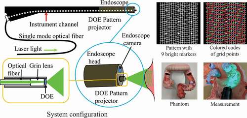
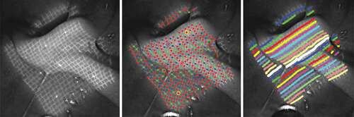
For this study, a projector-camera system was constructed by inserting a fibre-shaped, micro-pattern projector into the instrument channel of a standard endoscope. We used a Fujifilm EG-590WR endoscope and a pattern projector with a diffractive optical element (DOE) to generate structured-light illumination. The pattern projector can be inserted into the endoscope’s instrument channel and patterns are projected from the projector to surfaces in front of the head of the endoscope (Figure 1). As shown in (Figure 1), we used a grid pattern that is robust against subsurface scattering Furukawa et al. (2016). All vertical edges are connected; horizontal edges have small gaps, representing code letters $S$, $L$ and $R$ as shown as coloured codes in (Figure 1) (top right), where red dots mean that the right and the left edges of the grid point have the same height (code letter $S$), blue means the left side is higher (code letter $L$), and green means the right is higher (code $R$).

Figure 1. System configurations, projected patterns, and the appearances of the phantom model that was used for experiments of this paper.

When the micro-projector is inserted into the instrument channel, the system is uncalibrated. In this situation, the correspondence estimation is done purely by GCN-calculated embedding.

3.2. Algorithm

The overview of the algorithm is shown in (Figure 2). First, projected patterns, which consist of grids with gapped lines, are detected. In this process, the grid structure is detected by ‘phase’ detection by U-Nets (Sec. 4.1). Also, codes embedded in grid points are detected by another U-Net (Sec. 4.2).

Figure 2. 3D reconstruction process with auto-calibration.

The detected grid is represented as a graph with node-wise code (Sec. 4.3). A GCN is applied to the graph to find node-wise correspondences. By using the correspondences, auto-calibration is done by RANSAC to cope with outliers. After auto-calibration, the estimated extrinsic parameters are used for shape reconstruction in the next step.

The 3D reconstruction step is processed similarly. Since the extrinsic parameter is estimated in the auto-calibration process, epipolar constraints are used in the node-wise correspondence estimation (Sec. 4.4). Also, the node-wise correspondences are upgraded to pixel-wise correspondences using phase information to obtain dense, pixel-wise depth information (Sec. 4.1).

Finally, pixel-wise 3D shapes are reconstructed by using the extrinsic parameters. Multiple shapes are integrated by ICP to reconstruct large areas.

4. Detailed algorithm of dense 3D reconstruction using U-net and GCN

4.1. Pixel-wise shape reconstruction for sparse projection pattern using U-net

In this paper, we extract phases of repetitive patterns for each pixel from the captured image for dense shape reconstruction. From an input image, we extract grid features by estimating pixel-wise ‘phases’ of the cycles of the repeating features as shown in Figure 3(a). We train U-Nets to output sinusoidal patterns with different phases. The advantages of this method are that the sinusoidal patterns are smooth and relatively easy to learn by U-Net. We estimate $sin$ and $cos$ of the repeating ‘phase’ values of the grid by U-Nets and estimate phase by atan2 operation of the $sin$ and $cos$ values. An example of the output results from U-Net and an example of predicting phase values are shown in Figure 3(b-g)

Figure 3. Estimation of phase values using U-Nets: (a) Input image. (b) U-Net output for sin of horizontal phases. (c) U-Net output for cos of horizontal phases. (d) Estimated horizontal phases. (e) U-Net output for sin of vertical phases. (f) U-Net output for cos of vertical phases. (g) Estimated vertical phases. (h) Regions representing grid points. These regions are obtained by segmentation of the images by discontinuities of (d) and (g).

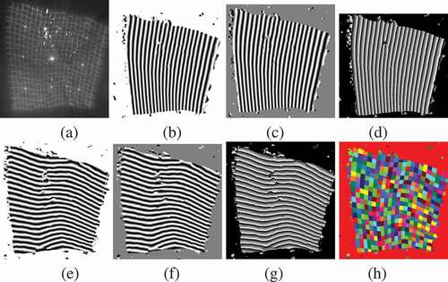
In the image of phase values of horizontal vertical directions, grid structure can be extracted by segmenting the regions with the discontinuity of these signals. We call each segmented region a superpixel Figure 3(h). By connecting those superpixels by adjacency, we can obtain a grid graph of the captured pattern.

For each grid point, the code information is assigned for the correspondence estimation described later. To extract the information, a U-Net that is trained to be applied to an input image and output code ID prediction is used. The information vectors are sampled from the output image of the U-Net. For the pattern of (Figure 1), three different codes are predicted. 1-hot vectors are constructed for each node are used as the feature vectors of the graph nodes.

Training of U-Net to perform phase and code estimation is achieved by supervised learning. In this paper, we generate training images by CG. Sinusoidal images with different phases that are synchronised with the original projection pattern are prepared. These images are projected on virtual 3D scenes. Similarly, correct code label IDs are drawn to CG images.

4.2. Building code-attributed graphs of detected features

As described previously, the projected pattern is a grid structure with code letters ($S/L/R$) associated with the grid points. We extract the grid structure and gap-code information by using U-Nets in the same method as Ronneberger et al. (2015).

In the paper, to add extra information to the feature vector of each node, we also add nine bright markers into the projected pattern as shown in (Figure 1) (top right) white dots. To utilise these markers in our method, we train CNNs to classify each of the markers into five classes (up to rotational symmetry, nine markers can be classified into five classes). By applying the trained CNNs, every pixel of the captured frames is classified into six classes (five plus one for non-marker).

In the output image from U-Net, the lines of the grid can be extracted as the boundaries between the regions to two labels. By performing the 8-neighbour labelling process on extracted boundary curves, different labels are assigned for each curve. Then, intersections between vertical and horizontal curves are extracted as grid points. By sorting the set of grid points on one vertical curve by $y$ coordinates, the adjacency relationships between these grid points along the vertical curve are determined. By applying this process for all of the vertical and horizontal curves, the grid structure of the extracted curves can be represented as a graph.

For each grid point, a feature vector is assigned using outputs of U-Net, such as 2D coordinates on the image, estimated code, and estimated marker class. (Figure 5) (left/middle) shows examples of an image and a graph extracted from the image. This attribute is embedded in feature vectors of 2 + 4 + 6 dimensions (2D coordinates, 4D code classes (three types for codes and one for unknown code), 6D marker classes (five types for markers and one for non-markers)).

4.3. GCN-calculated embedding of detected features

Once the code-attributed grid graph is detected from the image, correspondences between the nodes of the detected graph and those of the original projected graph are estimated.

Each grid point of the detected graph is attributed with a code of three alphabets, $\{S,L,R\}$. Although a single grid point is not enough for estimating correspondence, combinations of the nearby grid points with code attributes can be enough for estimating correspondences.

In this paper, we calculate node-wise feature embedding by using Graph Convolutional Network (GCN) Defferrard et al. (2016). A feature embedding of a single grid point is a compressed representation of codes, markers, and positional information of nearby grid points. The GCN is trained so that a simple cosine similarity function can be used for matching the detected grid graph and the original projected graph. The architecture of the GCN for calculating feature embedding is shown in (Figure 4).

Figure 4. Network architecture of GCN for calculating node-wise code-feature embedding.

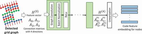
Figure 5. Training data for GCN:(left) a sample image;(middle) a grid detection result; (right) annotated column ID.

In Furukawa et al. (2016), the correspondences were estimated using both code information and epipolar constraints. However, if the extrinsic parameters of the projector are unknown or have large errors, the epipolar constraint cannot be used. To deal with this problem, we separated the matching measure into graph similarity measure and epipolar-constraint measure. The graph similarity measure represents the similarities between nodes of two graphs, and the epipolar-constraint measure represents the fulfilment of epipolar constraints between the nodes. Correspondences of the nodes are estimated by the weighted sum of those two measures. This strategy can be applied both with unknown or known extrinsic parameters. For a system with unknown extrinsic parameters, the weight of the epipolar-constraint measure can be set to zero. Once the correspondences are estimated, auto-calibration can be processed. Then, the correspondences can be re-estimated using the calibrated extrinsic parameters as shown in (Figure 2).

As shown in (Figure 4), the layer operation of a GCN is applied to a data matrix $H^{(l)}$, where the $l$-th layer feature vectors of all the grid points are stacked to one matrix of $N\times 12$, where $N$ is the number of the grid points and 12 is the dimension of feature vectors (2D for relative positional information, 4D for code information including unknown, and 6D for marker information including unknown). The operation produces $H^{(l+1)}$, which is the $(l+1)$-th layer data matrix. It can be represented as

$H^{(l+1)}=f(H^{(l)},A,W^{(l)})=\sigma ({\hat{D}}^{-1/2}\hat{A}{\hat{D}}^{-1/2}{H}^{(l)}{W}^{(l)})$

where $\hat{A}=A+I$ is the adjacency matrix of graph $G$ with added self-connections, $I$ is the identity matrix, $\hat{D}$ is the degree matrix of $\hat{A}$, $W^{(l)}$ is the Weight matrix of this layer, and $\sigma$ is an activation function (ReLU).

In Defferrard et al. (2016), the network is an undirected graph, but in the case of this research, the information of a grid point can be obtained from adjacent nodes of 4 directions of top, bottom, right and left, and information from different directions has different meanings. Thus, for treating the four directions differently, we set $A_0,A_1,A_2,A_3$ as the adjacency matrix of the directed graph that includes only the connections of top, bottom, right, and left directions, respectively. Calculation of $H^{(l+1)}$ is performed by the following formula.

(1) $H^{(l+1)}=\sum _{d=0}^{3}f(H^{(l)},A_d,W_d^{(l)})$(1)

where $W_d^{(l)}$ is the weight matrix of layer $l$ specific to direction $d\in \{0,1,2,3\}$.

After repeating Equation (1)(1) $H^{(l+1)}=\sum _{d=0}^{3}f(H^{(l)},A_d,W_d^{(l)})$(1) and batch normalisation by 5 times, $D_e$ dimensional feature embeddings are calculated from $H^{(5)}$ by a fully connected linear transformation.

Both the detected grid graph ${\mathbf{G}}_d$ and the projected grid graph ${\mathbf{G}}_p$ are processed with the same GCN, producing a feature embedding matrix of ${\mathbf{F}}_d$ with size $N_d\times D_e$, and ${\mathbf{F}}_p$ with size $N_p\times D_e$, where $N_d$ and $N_p$ are the numbers of grid points of ${\mathbf{G}}_d$ and ${\mathbf{G}}_p$. Then ${\mathbf{F}}_d{\mathbf{F}}_p^{\mathrm{T}}$ becomes the matrix with cosine similarities of the feature embeddings between the nodes of these graphs. By taking argmax(softmax(${\mathbf{F}}_d{\mathbf{F}}_p^{\mathrm{T}}$)) where argmax and softmax are row-wise, we can estimate the mapping from nodes of the detected grid graph to nodes of the projected pattern graph.

Training of the GCN is done in a supervised manner. First, a graph structure is extracted from an actual endoscopic image using U-Net. Separately, for the same endoscopic image, the class IDs of both vertical and horizontal lines are manually annotated as shown in (Figure 5) (right), which are used as teacher data. The GCN is trained by using the cost function of cross-entropy between softmax (${\mathbf{F}}_d{\mathbf{F}}_p^{\mathrm{T}}$) and the teacher data labels.

4.4. Correspondence estimation using epipolar constraints

In the proposed system, the correspondence estimation can be done both with and without epipolar constraints. If the extrinsic parameters are known, epipolar constraints are taken into account.

The approach is simple. The similarity measure matrix ${\mathrm{M}}_s$ is defined to be softmax (${\mathbf{F}}_d{\mathbf{F}}_p^{\mathrm{T}}$). It includes similarities for all the node pairs between ${\mathbf{G}}_d$ and ${\mathbf{G}}_p$. For each of the pairs, an epipolar constraint can be calculated. Let the distance between the epipolar line of $j$-th node of ${\mathbf{G}}_p$ and the 2D position of $i$-th node of ${\mathbf{G}}_d$ be $Dist(i,j)$, then the epipolar constraint measure matrix $M_e$ is defined by

(2) $({\mathrm{M}}_e{)}_{i,j}\equiv -\{max(Dist(i,j)-T_e,0){\}}^2$(2)

where $T_e$ is the margin of epipolar constraints so that epipolar-constraint errors that are smaller than $T_e$ do not affect the measurement.

Then, the total measure ${\mathrm{M}}_t$ is

(3) ${\mathrm{M}}_t\equiv {\mathrm{M}}_s+w_e{\mathrm{M}}_e$(3)

where $w_e$ is the weight for the epipolar constraints. The correspondences are estimated by row-wise argmax of ${\mathrm{M}}_t$. Epipolar constraints can be switched on and off by setting $w_e$ to a plus value and zero.

4.5. Auto-calibration of the projector and 3D reconstruction

In the proposed system, we assume that the extrinsic parameters are not known, because medical doctors can freely insert the projector into the endoscope and capture the image. Thus, we auto-calibrate the extrinsic parameters as shown in (Figure 2).

First, correspondences are estimated with $w_e=0$. Then, the extrinsic parameters are estimated so that the epipolar constraints are fulfilled. To deal with outlier correspondences, the RANSAC algorithm is used.

In this process, we use a model of projector pose proposed in Furukawa et al. (2015), where most of the projector pose is explained as one-dimensional translation along the instrument channel and rotation about the centre-line of the channel. Such restriction also allows the scale to be determined, which is normally impossible for auto-calibration, and leads to stabilisation of the auto-calibration.

After extrinsic parameters are estimated, correspondences are estimated with $w_e$ to be a plus value so that the epipolar constraints are taken into account. These correspondences are used for 3D reconstruction.

5. Experiments

We implemented the proposed method and trained the GCN using 49 images of real bio-tissues and a phantom model that is not the phantom in (Figure 1). $D_e=96$ and $N_p=21\times 21$. The intermediate dimensions between the GCN layers were all 96. Then, we captured images of the colon phantom shown in (Figure 1) and processed the correspondence estimation. For evaluation, we manually annotated ground-truth correspondences, similarly in making the training data for the GCN.

We compared the proposed method with LBP Felzenszwalb and Huttenlocher (2006). LBP is processed on graph ${\mathbf{G}}_d$. Data cost was defined by using the node-wise match of codes between ${\mathbf{G}}_d$ and ${\mathbf{G}}_p$, and regularisation cost was defined by using the adjacencies of ${\mathbf{G}}_p$. In this experiment, we applied three iterations for the LBP-based correspondence estimation.

(Figure 7) shows the correspondence estimation results for sample image A. (Figure 6) shows the result of auto-calibration and the depth estimation. And the accuracy rates of correspondence estimation are shown in (Table 1). The execution times in CPU implementation for the correspondence estimation was about 0.09 seconds for the proposed method, and about 0.6 seconds for LBP.

Figure 6. Auto-calibration and depth estimation results of sample image A. The first and second images show epipolar lines of bright markers. The bright markers should be on the epipolar lines. Depth estimation is visualised with heat map colours.

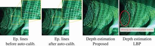
Table 1. Accuracy rates of correspondence estimation.

	Proposed,	LBP,	Proposed,	LBP,	Direct ID prediction
	${\mathrm{M}}_s$	${\mathrm{M}}_s$	${\mathrm{M}}_s+w_e{\mathrm{M}}_e$	${\mathrm{M}}_s+w_e{\mathrm{M}}_e$	Furukawa, et al., (2020)
Sample A	0.909	0.760	0.986	0.819	0.917
Sample B	0.857	0.904	0.981	0.948	0.817
Sample C	0.634	0.641	0.777	0.741	0.607

The results show that the proposed method is comparable or outperforms LBP, while the execution time was significantly smaller. Since LBP explicitly models the continuity of matching nodes of graphs, LBP tends to perform better for continuous graphs. On the other hand, GCN-calculated embedding tends to be more robust against discontinuities of the graphs. LBP sometimes makes mistakes for multiple adjacent nodes in a certain area at the same time, as can be seen in (Figure 7). Both results of the proposed method and LBP were improved by the additional epipolar constraints after auto-calibration (Figure 7 and Table 1: ${\mathrm{M}}_s$ vs. ${\mathrm{M}}_s+w_e{\mathrm{M}}_e$).

Figure 7. Correspondence estimation results of sample image A, using the proposed method and LBP Felzenszwalb and Huttenlocher (2006). Blue/red dots in correspondence accuracy images mean correct(blue)/incorrect(red) correspondence estimations.

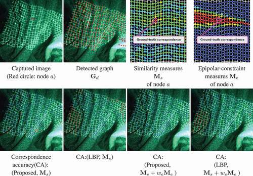
In (Table 1), the correspondence accuracies obtained by using the method of. (Furukawa, et al., 2020) are also compared with the proposed method. This method does not use the similarity calculation instead, directly predicts the node IDs using a GCN. Specifically, the method iterates 21 classification problems of the node ID estimation for each column and row, respectively. The result of Sample A shows that, without the epipolar constraint, the accuracy rate of the proposed method (0.909) is slightly lower than the method. (Furukawa, et al., 2020) (0.917). The epipolar constraint improves correspondence accuracy in the proposed method (0.986). In addition, the proposed method outperforms in Sample B and Sample C, which shows that the similarity calculations is more stable than the direct estimation method.

(Figure 8) shows reconstruction results of a stomach phantom. The same captured images were constructed with the proposed method and a baseline method of Furukawa et al. (2015), where line-based shapes are interpolated with radial basis function. The figures show that the proposed method outperformed in the quality of the detailed shapes. Since the shapes are dense, multiple shapes from image sequences can be easily registered using ICP. (Figure 9) shows the registered shapes.

Figure 8. The reconstruction results of the proposed method and Furukawa et al. (2015): (a)-(c):Captured images. (d)-(f):Reconstruction results of the proposed method for inputs of (a-c). (g)-(i):Reconstruction results of Furukawa et al. (2015) for inputs of (a-c).

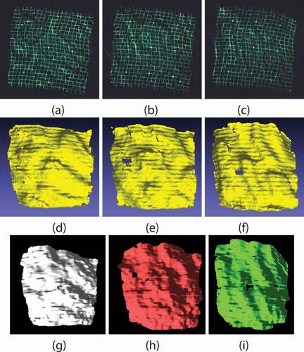
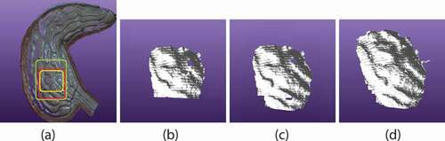
Figure 9. Results of multiple scan integration: (a) overview of phantom of stomach, (b) single scan result, which is indicated by yellow rectangle in (a), (c) two shapes integration result indicated by red rectangle, and (d) five shapes integration result indicated by green. Because of our auto-calibration method, shapes are consistently recovered and it is confirmed that multiple shapes are successfully registered and integrated.

6. Conclusion

In this paper, we propose a one-shot, dense active-stereo method using a static pattern consisting of lines and dots. From a captured image, pixel-wise phase information of the projected pattern is obtained as a phase-grid image. The image is segmented with superpixels (sub-regions with single phase-cycles for vertical and horizontal directions) and formed into a grid graph. By using GCN-based correspondence estimation, node-wise correspondences are obtained. By using the correspondences and the phase information, auto-calibration and dense 3D shapes estimation are achieved. In addition, since reconstructed shapes are consistent, ICP is robustly applied to integrate multiple scanning results to generate large 3D shapes. In the future, an integration technique for non-rigid objects is important for medical purposes.

Disclosure statement

No potential conflict of interest was reported by the author(s).

Additional information

Funding

This work was supported by JSPS JP20H00611, JP18H04119 NEDO (New Energy and Industrial Technology Development Organization) JPNP20006 in Japan.

References

- Defferrard M, Bresson X, Vandergheynst P. 2016. Convolutional neural networks on graphs with fast localized spectral filtering. In: Advances in neural information processing systems. p. 3844–3852. https://papers.nips.cc/.
- Felzenszwalb PF, Huttenlocher DP. 2006. Efficient belief propagation for early vision. Int J Comput Vis. 70(1):41–54. doi:10.1007/s11263-006-7899-4.
- Furukawa R, Masutani R, Miyazaki D, Baba M, Hiura S, Visentini-Scarzanella M, Morinaga H, Kawasaki H, Sagawa R. 2015. 2-dof auto-calibration for a 3d endoscope system based on active stereo. In: 2015 37th Annual International Conference of the IEEE Engineering in Medicine and Biology Society (EMBC). Milan, Italy; IEEE. p. 7937–7941.
- Furukawa R, Mizomori M, Hiura S, Oka S, Tanaka S, Kawasaki H. 2018. Wide-area shape reconstruction by 3d endoscopic system based on cnn decoding, shape registration and fusion. In: or 2.0 context-aware operating theaters, computer assisted robotic endoscopy. In: clinical image-based procedures, and skin image analysis. Cham: Springer; p. 139–150.
- Furukawa R, Morinaga H, Sanomura Y, Tanaka S, Yoshida S, Kawasaki H. 2016. Shape acquisition and registration for 3d endoscope based on grid pattern projection. In: European Conference on Computer Vision Amsterdam, The Netherlands; Cham: Springer. p. 399–415.
- Furukawa R, Oka S, Kotachi T, Okamoto Y, Tanaka S, Sagawa R, Kawasaki H. 2020. Fully auto-calibrated active-stereo-based 3d endoscopic system using correspondence estimation with graph convolutional network. In: 2020 42nd Annual International Conference of the IEEE Engineering in Medicine & Biology Society (EMBC) EMBS Virtual Academy; IEEE. p. 4357–4360.
- Geurten J, Xia W, Jayarathne U, Peters TM, Chen EC. 2018. Endoscopic laser surface scanner for minimally invasive abdominal surgeries. In: International Conference on Medical Image Computing and Computer-Assisted Intervention; Granada, Spain: Springer. p. 143–150.
- Ikeuchi K, Matsushita Y, Sagawa R, Miyazaki D, Mukaigawa Y, Furukawa R, Kawasaki H. 2020. Active lighting and its application for computer vision –40 years of history of active lighting techniques. Cham: Springer.
- Kawasaki H, Furukawa R, Sagawa R, Yagi Y. 2008. Dynamic scene shape reconstruction using a single structured light pattern. In: Proceedings of the IEEE Conference on Computer Vision and Pattern Recognition (CVPR) Anchorage, Alaska, USA; Ieee. p. 1–8.
- Liu X, Sinha A, Unberath M, Ishii M, Hager GD, Taylor RH, Reiter A. 2018. Self-supervised learning for dense depth estimation in monocular endoscopy Stoyanov, Danail. In: Or 2.0 context-aware operating theaters, computer assisted robotic endoscopy, clinical image-based procedures, and skin image analysis. Cham: Springer; p. 128–138.
- Ma R, Wang R, Pizer S, Rosenman J, McGill SK, Frahm JM. 2019. Real-time 3d reconstruction of colonoscopic surfaces for determining missing regions. In: International Conference on Medical Image Computing and Computer-Assisted Intervention Shenzhen, China; Springer. p. 573–582.
- Mahmood F, Chen R, Durr NJ. 2018. Unsupervised reverse domain adaptation for synthetic medical images via adversarial training. IEEE Trans Med Imaging. 37(12):2572–2581. doi:10.1109/TMI.2018.2842767.
- Mahmood F, Durr NJ. 2018. Deep learning and conditional random fields-based depth estimation and topographical reconstruction from conventional endoscopy. Med Image Anal. 48:230–243. doi:10.1016/j.media.2018.06.005.
- Maurice X, Albitar C, Doignon C, de Mathelin M. 2012. A structured light-based laparoscope with real-time organs’ surface reconstruction for minimally invasive surgery. In: 2012 Annual International Conference of the IEEE Engineering in Medicine and Biology Society. San Diego, CA, USA; IEEE. p. 5769–5772.
- Nagakura T, Michida T, Hirao M, Kawahara K, Yamada K. 2006. The study of three-dimensional measurement from an endoscopic images with stereo matching method. In: 2006 World Automation Congress Budapest , Hungary; IEEE. p. 1–4.
- O’Toole M, Achar S, Narasimhan SG, Kutulakos KN. 2015. Homogeneous codes for energy-efficient illumination and imaging. ACM Trans Graph. 34(4):35:1–35:13. Available from: doi:10.1145/2766897.
- Rau A, Edwards PE, Ahmad OF, Riordan P, Janatka M, Lovat LB, Stoyanov D. 2019. Implicit domain adaptation with conditional generative adversarial networks for depth prediction in endoscopy. Int J Comput Assist Radiol Surg. 14(7):1167–1176. doi:10.1007/s11548-019-01962-w.
- Ronneberger O, Fischer P, Brox T. 2015. U-net: convolutional networks for biomedical image segmentation. In: International Conference on Medical Image Computing and Computer-Assisted Intervention Munich, Germany; Springer. p. 234–241.
- Salvi J, Pages J, Batlle J. 2004. Pattern codification strategies in structured light systems. Pattern Recognit. 37(4):827–849. doi:10.1016/j.patcog.2003.10.002.
- Schmalz C, Forster F, Schick A, Angelopoulou E. 2012. An endoscopic 3d scanner based on structured light. Med Image Anal. 16(5):1063–1072. doi:10.1016/j.media.2012.04.001.
- Song L, Tang S, Song Z. 2017. A robust structured light pattern decoding method for single-shot 3d reconstruction. In: 2017 IEEE International Conference on Real-time Computing and Robotics (RCAR) Okinawa, Japan; IEEE. p. 668–672.
- Stoyanov D, Scarzanella MV, Pratt P, Yang GZ. 2010. Real-time stereo reconstruction in robotically assisted minimally invasive surgery. In: International Conference on Medical Image Computing and Computer-Assisted Intervention Beijing, China. Springer. p. 275–282.
- Visentini-Scarzanella M, Sugiura T, Kaneko T, Koto S. 2017. Deep monocular 3d reconstruction for assisted navigation in bronchoscopy. Int J Comput Assist Radiol Surg. 12(7):1089–1099. doi:10.1007/s11548-017-1609-2.
- Wang J, Sankaranarayanan AC, Gupta M, Narasimhan SG. 2016. Dual structured light 3d using a 1d sensor. In: Computer Vision - ECCV 2016-14th European Conference; Amsterdam, The Netherlands, Oct 11-14, Proceedings, Part VI. p. 383–398. doi: 10.1007/978-3-319-46466-4_23.
- Zagoruyko S, Komodakis N. 2015. Learning to compare image patches via convolutional neural networks. In: Proceedings of the IEEE Conference on Computer Vision and Pattern Recognition. Boston, Massachusetts, USA. p. 4353–4361.
- Žbontar J, LeCun Y. 2016. Stereo matching by training a convolutional neural network to compare image patches. J Mach Learn Res. 17(1):2287–2318.
- Zhang L, Curless B, Seitz SM. 2002. Rapid shape acquisition using color structured light and multi-pass dynamic programming. In: Proceedings First International Symposium on 3D Data Processing Visualization and Transmission. Padova, Italy; IEEE. p. 24–36.
- Zhang Z. 2012. Microsoft kinect sensor and its effect. IEEE MultiMedia. 19(2):4–12. Available from: https://www.microsoft.com/en-us/research/publication/microsoft-kinect-sensor-and-its-effect.