Optimization of deep neural networks for multiclassification of dental X-rays using transfer learning

ABSTRACT

In this work, the segmented dental X-ray images obtained by dentists have been classified into ideal/minimally compromised edentulous area (no clinical treatment needed immediately), partially/moderately compromised edentulous area (require bridges or cast partial denture) and substantially compromised edentulous area (require complete denture prosthesis). A total of 116 image dental X-ray dataset is used, of which 70% of the image dataset is used for training the convolutional neural network (CNN) while 30% is used sfor testing and validation. Three pretrained deep neural networks (DNNs; SqueezeNet, ResNet-50 and EfficientNet-b0) have been implemented using Deep Network Designer module of Matlab 2022. Each of these CNNs were trained, tested and optimised for the best possible accuracy and validation of dental images, which require an appropriate clinical treatment. The highest classification accuracy of 98% was obtained for EfficientNet-b0. This novel research enables the implementation of DNN parameters for automated identification and labelling of edentulous area, which would require clinical treatment. Also, the performance metrics, accuracy, recall, precision and F1 score have been calculated for the best DNN using confusion matrix.

KEYWORDS:

• Convolutional neural network
• deep neural network
• image classification
• edentulous

1. Introduction

Edentulous patients exhibit a wide range of physical differences and health issues. Classifying these edentulous patients as a single group is not justified as there are multiple levels of treatment procedure dependent on the extent of physical damage, which requires restoration of comfort or function. McGarry et al. (1999) proposed a classification system for complete edentulism, wherein they were classified according to specific diagnostic criteria but had not implemented computational tools available in machine learning (ML) or deep learning network for classification. As there are no organised criteria for diagnosis of complete edentulism, this has prevailed as a great obstacle preventing the delivery of efficient care for patients. Although the dental literature defines methods to recognise the degree of edentulism, diverse nature and its scope, these methods are not organised effectively to guide the dental professional, prosthodontists etc., for providing specific treatment for each patient. Hence, the patient identification is essential for improving the outcomes of dental treatment.

Recently, dental informatics have received significant attention in the field of dentistry that has inherently improved diagnostics and treatment quality while also reducing the fatigue and stress involved in everyday practice. Dental imaging (X-rays) generate a vast amount of data from various sources such as biosensors and high-resolution imaging (Shah 2014). Dentists can benefit from various computer-based algorithms for their decision-making such as treatment planning (Masic 2012). In a clinical set-up, deep learning has already been implemented for treatments (Nair et al. 2021). The success of the deep learning method is mainly due to computational tool advances, new methods and enormous data.

During the last few years, deep learning methods have gained a lot of attention. Convolutional neural networks (CNNs) have been extensively implemented for medical image analysis due to their fast development. Eye exams for diabetic retinopathy and clinical skin screenings have successfully employed CNNs (Rathod et al. 2018). Researchers have recently widely examined the implementation of CNNs and deep learning to understand numerous kinds of medical images, with great results (Bhalla et al. 2022). In recent years there has been a significant rise in diagnosing disease using deep learning techniques, which has further improved the clinical treatment quality for patients. It is important to note that the use of deep convolutional networks in dentistry has been done since 2015.

Computer-based segmentation of images in dentistry has been introduced using various methods (Singh and Kaur 2020, 2021). Image classification and object detection are two examples of computer vision problems used by deep learning (Leonard 2019). A growing use of deep learning-based algorithms has recently been becoming popular for image segmentation. Full-connected networks (FCNs) are a common approach for segmentation, which has been applied to numerous image-processing applications (Girshick et al. 2014). The implementation of Fully Convolutional Network (Long et al. 2015) led to end-to-end segmentation of image and significantly exceeded in performance in comparison to traditional segmentation algorithms in precision. In recent years, the research on the CNN structure is popularised, and few CNN networks with outstanding performance have been implemented (Simonyan and Zisserman 2015; Szegedy et al. 2015; He et al. 2016). Furthermore, with the effective implementation of transfer learning applied to CNN, the domain-specific application of CNNs has been further extended to other fields of engineering and medicine (Collobert et al. 2011; Oquab et al. 2014). A detailed review of the different methodologies employed, databases used, results obtained and drawbacks observed in research works related to dental image classification using deep learning and ML techniques is provided in Table 1. From the literature review, to the best of the authors’ knowledge, it is found that classification of edentulous condition of the mandible has not been investigated by other researchers.

Table 1. Previous works related to dental image classification.

Author (Year)	Methodology	Database	Results	Drawbacks
(Prajapati et al. 2017)	Transfer learning-based CNN with five convolutional, two maximum pooling and four Fully Connected layers	251 labelled images from an undisclosed source	Best accuracy of 88.46% in classifying the dental images as ‘dental caries disease’, ‘periapical infection’ and ‘periodontitis’	1. Effect of batch size and solver type not investigated 2. Data augmentation not conducted 3. Only one deep learning model employed
Wijaya (2018)	Naïve Bayes method	Not disclosed	Best accuracy of 66.6% in classifying different dental abnormalities	1. DNNs such as ResNet and EfficientNet not compared 2. Effect of batch size and solver type not investigated 3. Data augmentation not conducted
(Yang et al. 2018)	CNN with four convolutional, two Fully Connected layers and a SoftMax layer	196 labelled periapical dental radiographs of the apical region from an undisclosed source	80% accuracy, 0.749 F1 score for classifying the images as ‘getting better’, ‘getting worse’ and ‘have no explicit change’	1. Effect of batch size and solver type not investigated 2. Only one deep learning model employed
(Sukegawa et al. 2020)	Five models were taken: A CNN with five convolutional layers, transfer-learning based VGG16 and VGG19 and fine-tuned VGG16 and VGG19 models	8859 radiographic images obtained from Kagawa Prefectural Central Hospital, Japan	Fine-tuned VGG16 showed best performance with 92.8% accuracy, 0.916 F1, Recall 0.907 and Precision 0.928 in classifying images into 11 types of implant systems	1. DNNs such as ResNet and EfficientNet not compared 2. Effect of batch size and solver type not investigated
(Sivasundaram and Pandian 2021)	A modified LeNet CNN with four convolutional, two maximum pooling and a fully connected layer	3513 panoramic dental images after data augmentation	99.63% Accuracy, F1 0.989, Precision 0.9975 for classifying the images as ‘dental cyst’, ‘periodontal bone defects’, ‘periapical lesions’ and ‘pathological jaw lesions’	1. Effect of batch size and solver type not investigated 2. Only one deep learning model employed
(Cejudo et al. 2021)	1. A baseline CNN with two convolutional, a ReLU function, a maximum pooling layer, two fully connected layer, ReLU and SoftMax function 2. ResNet-34 pretrained on ImageNet and CapsNet	90,388 radiographs from Charité–Universitätsmedizin Berlin, Germany (Charité) and King George’s Medical University (KGMU), Lucknow, India	ResNet showed significantly better performance with 99.7% accuracy, 0.991 F1 and 0.996 Precision in classifying the images as ‘panoramic’, ‘bitewing’, ‘periapical’ and ‘cephalometric’	1. Transfer learning was only applied to ResNet 2. Effect of batch size and solver type not investigated
(Jusman et al. 2021)	Support Vector Machine (SVM) and K-Nearest Neighbors (KNN)	396 pre-labelled images obtained from the Dental and Oral Hospital (RSGM) of Universitas Muhammadiyah Yogyakarta, Indonesia	Fine Gaussian SVM showed best performance with 95.7% accuracy in classifying the images into four classes of dental caries	1. DNNs not explored 2. Effect of batch size and solver type not investigated
(Liu et al. 2020)	Mask Region-based CNN (R-CNN)	12,600 clinical images collected from 10 private dental clinics in China	Accuracy up to 90% for predicting seven classes of dental diseases	1. Effect of batch size and solver type not investigated 2. Data augmentation not conducted 3. Only one deep learning model employed
(Lee et al. 2018)	GoogLeNet Inception v3 CNN network model	3000 periapical radiographic images obtained from Department of Periodontology, Daejeon Dental Hospital, Wonkwang University	Overall accuracy about 86.33% for the detection of dental caries in premolars and molars	1. Effect of batch size and solver type not investigated 2. Only one deep learning model employed
(Bouchahma et al. 2019)	A CNN model with four convolutional, three maximum pooling, one flattened and one fully connected layer	120 periapical X-ray images from top to bottom jaw obtained from Rad et al. (2016)	Overall accuracy of 86% for classifying the images as ‘no treatment’, ‘fluoride’, ‘filling’ and ‘root canal’	1. Effect of batch size and solver type not investigated 2. Data augmentation not conducted 3. Only one deep learning model employed
(Moutselos et al. 2019)	Mask Region-based CNN (R-CNN)	88 intra-oral camera images were obtained from patients that were treated at the Paediatric Dentistry Clinic of the Dental School of the National and Kapodistrian University, Athens, Greece	F1 score around 0.6 for predicting seven levels of severity of caries disease. For most severe classes, the accuracy was around 0.8	1. Only one deep learning model employed 2. Effect of batch size and solver type not investigated
(Geetha et al. 2020)	Feed-forward backpropagation neural network with one hidden layer	105 intra-oral digital radiographs obtained from SJM Dental College Chitradurga, India	Accuracy close to 97% in identifying the caries disease	Did not address a multi-class problem (only two classes)
(Rana et al. 2017)	CNN consisting of convolutional, maximum pooling, upsampling, rectified linear unit and final sigmoid activation	405 colour-augmented images obtained from 150 individuals during a study at the 2015 Kumbh Mela in Nashik, India	Area under receiver-operating characteristic (ROC) curve of 0.746, 0.347 precision and 0.621 recall for automatic identification of inflammation regions due to gingival disease	1. Only one deep learning model employed 2. Effect of batch size and solver type not investigated
(Krois et al. 2019)	CNN with convolutional layers, ReLU activation function and maximum pooling layers	350 panoramic dental radiographs obtained from Universität Düsseldorf, Germany, which was split into 1750 image segments	Classification accuracy of 81% for detection of periodontal bone loss	1. Only one deep learning model employed 2. Effect of batch size and solver type not investigated
(You et al. 2020)	A DeepLabV3+ CNN model	886 intraoral photos obtained from 86 children aged 5 to 8 years undergoing dental treatment at the Department of Pediatric dentistry, Peking University School and Hospital of Stomatology in Beijing, China	Accuracy around 72.6% for dental plaque detection on primary teeth	1. Only one deep learning model employed 2. Effect of batch size and solver type not investigated
(Tian et al. 2019)	3D CNN	600 dental models extracted from the scanned dentition plaster models	Classification of type of teeth as ‘incisor’, ‘canine’, ‘premolar’ and ‘molar’ with 95.96% accuracy, and 2-label classification of the tooth category with 88.06% accuracy	1. Only one deep learning model employed 2. Effect of batch size and solver type not investigated
(Laishram and Thongam 2020)	Faster-Regional Convolutional Neural Network (Faster-RCNN)	145 images from an undisclosed clinic	Accuracy of more than 90% for detection and 99% for classification of teeth as ‘incisor’, ‘molar’, ‘premolar’ and ‘canine’	1. Only one deep learning model employed 2. Effect of batch size and solver type not investigated
(Imangaliyev et al. 2016)	CNN model with maximum pooling layers, one fully connected layer followed by a multinomial logistic regression function	427 Quantitative Light-induced Fluorescence (QLF) images obtained from the Department of Preventive Dentistry of Academic Centre for Dentistry, Amsterdam, The Netherlands	0.75 ± 0.05 F1-score	1. Only one deep learning model employed 2. Effect of batch size and solver type not investigated
(Salunke et al. 2022)	A customised CNN model with six convolutional layers	1336 X-ray images collected from the Tirupati Dental Clinic, Pune, India	Average precision of 94.59%, recall of 95.89%, F1-score of 94% and average testing accuracy of 94.2 %	1. Only one deep learning model employed 2. Effect of batch size and solver type not investigated
(Ilić et al. 2019)	Transfer learning aided pretrained VGG16 CNN model	4155 images provided by School of Dental Medicine, University of Zagreb, Croatia	Accuracy of 94.3%	Effect of batch size and solver type not investigated
(Al-Ghamdi et al. 2022)	AlexNet, CNN and NASNet models	Unidentified and anonymised panoramic dental X-ray images of a total of 116 patients, acquired from Noor Medical Imaging Center, Qom, Iran	Accuracy around 96%	Effect of batch size and solver type not investigated

2. Fundamentals of image classification

An artificial neural network (ANN) is referred to a traditional neural network, which is implemented widely in artificial intelligence. ANN utilises neurons of the network to understand the attributes of external things, which is to be further processed by the computer for completing the data processing.

ANN designs the network structure in accordance with the various construction methods of neurons. In general, a neural network is regarded as an operational model consisting of numerous different neurons connected with each other. Each of these nodes becomes a processing function, and the connection between them employs weight to signify the memory capacity of ANN. The output of ANN relies on the weight value, connection form and excitation function of different nodes. It should be noted the neural network model is mainly constructed with respect to some function or algorithm that expresses certain logical operation.

Neurons represent a transformation or an operation, which is completed by the activation function of neurons. Two adjacent layers of neurons are connected to each other, as shown in Figure 1. A simple neural network consists of information as follows: input layer, hidden layer and output layer. Each of these layers consists of numerous neurons (Bhat and Deepak 2023). Neurons basically represent operation or transformation that is completed using activation function. The successive adjacent layer of neurons is connected as shown in Figure 1.

Figure 1. Connections between neurons in different layers.

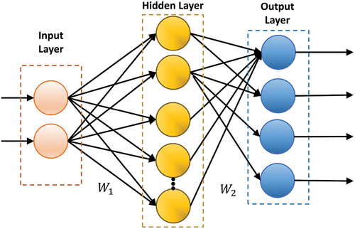
As can be seen from Figure 1, the neural network model includes 11 neurons: three input layers, five hidden layers and three output layers. +e structure belongs to a two-layer neural network model, where W1 and W2 are the weight matrices of the hidden layer and the output layer, respectively. As depicted in Figure 1, the neural network architecture comprises 11 neurons (three input, five hidden and three output layers); the architecture represents a two-layer neural network, where W1 and W2 are matrices of weight of the hidden and output layers.

Deep learning method is a component of ML. It is broadly implemented in image classification, language recognition and image detection. Deep learning has been developed from ANN theory. By inferring the human brain for hierarchic information processing, various layer levels of neural networks have been developed. Deep learning is very effective in the extraction of multiple features of information by mimicking the human brain to obtain important features of text, image and other data types. Deep learning mostly describes a particular set of object attributes via hierarchic processing in accordance with large edge feature information. The process follows feature extraction from low-level to higher-level combinations. It is imperative to understand that deep learning is an efficient tool to process huge data and retrieve abstract features using a neural network model.

Deep learning comprises multiple layers of deep neural network (DNN). In accordance with the connection of neurons in the human brain, the extracted features are analysed in different layers of model and this yields the deep features of the sample data. Comparable to DNN, the ANN also belongs to hierarchic structure for processing information. The model consists of a multilayer perceptron that includes input, hidden and output layers. Unlike deep network model, the ANN only consists of 2–3 layers of forward neural network, and the number of neurons in each layer is relatively very small, thereby limiting the processing capacity for huge datasets. As the DNN model has numerous layers, each of these layers contain large number of neurons, which enable them to have a strong learning function essential to understand the abstract expression of data.

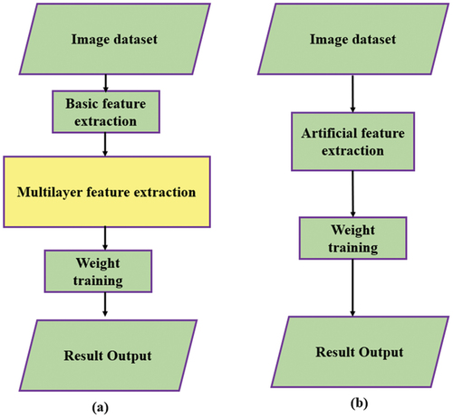
In comparison to the traditional ML methods, the deep learning method is not dependent on the feature extraction and manual design. In addition to solving knowledge shortage issue, it also eliminates the priority issue in feature extraction. Also, the deep learning model obtains high-level features via a combination of low-level features (Ma et al. 2022). Information process flow in traditional neural network and DNN is shown in Figure 2.

Figure 2. Information process flow in (a) deep learning algorithm and (b) traditional ML algorithm.

Typically, in a neural network, the activation function is implemented to perform nonlinear computing of input data of neurons to effectively retrieve the feature information from the input data. Activation function is a nonlinear function. With augmentation in number of layers of the neural network, the most important feature information could be extracted only after numerous data training and iterations.

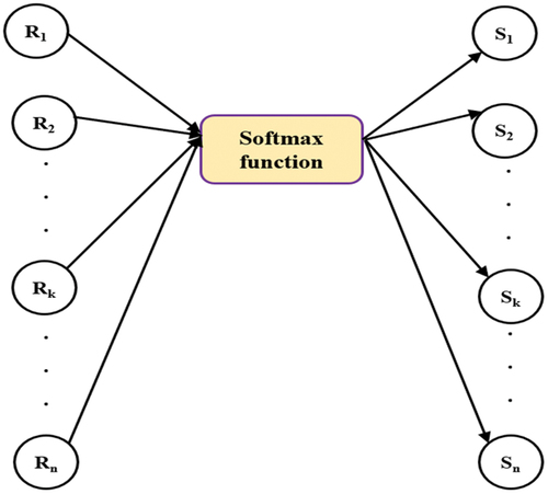
In order to image classification, most commonly the Softmax activation function is implemented in the neural network model and used as the output layer. The computation formula is

(1) $S_k=\frac{exp\left(R_k\right)}{{\sum }_{k=1}^{n}exp\left(R_k\right)}$(1)

where n is the number of neurons and Rk is the nonlinear transformation value in the kth neuron in this layer.

Softmax is implemented as the output for various feature groups. The corresponding neuron value obtained in each layer is considered as the probability of that category. The calculation process of Softmax function is shown in Figure 3.

Figure 3. Softmax function for calculation.

3. Fundamentals of CNN

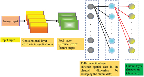
CNN is a typical network structure in deep learning model (He et al. 2016). Different from traditional ML, a CNN can be better used for image and time-series data processing, especially for image classification and language recognition. CNN Structure (CNNS) is network type in deep learning method (Guo et al. 2018). Unlike traditional ML, CNNS is specifically suited for time-series processing of data, particularly language recognition and image processing and specifically image classification. The structure of CNNS is seen in Figure 4.

Figure 4. Basic structure of CNNs.

The CNNS comprises three different processing layer types: convolution layer, pooling layer and full connected layer. Among these, the feature extraction is implemented using convolution layer, while the mapping of features is done via pooling layer. The fully connected layer is similar to neural network architecture. Every node in this fully connected layer is not connected to each other, while it is completely connected to all nodes of the previous layer. Similar to neural network, the CNNS also has an input layer for data and an output layer for results.

The computing of CNN is predominantly done by convolution layer and also via convolution kernel present in the convolution layer that forms the core of the CNN model. The convolution layer implements the convolution check to convolute the input image and retrieve the distinctive information of the image. Furthermore, the images processed via convolution operator will reduce to smaller size, and pixels at the image edge will have no impact on the results of the output.

As seen in Figure 5, assuming input image as a 3 × 3 matrix, the original is convoluted via a 2 × 2 size convolution check and the feature map is the output.

Figure 5. Schematic of the convolution process.

In general, there is a strong connection between adjacent pixels of an image. The convolution kernel essentially retrieves characteristics/features of particular localised area of the image and sends these retrieved features to higher level of integration processing.

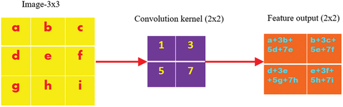
As the bottom feature of the image is not dependent on its position, it would not be able to apply the same convolution check for retrieval of relevant characteristics/features; although it also reduces the number of neural network parameters via the shared weight characteristic of convolution kernel, it is inherently done for the improvement of training efficiency of the network model.

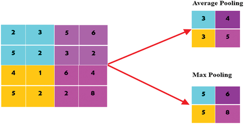
For complex images, in order to reduce the amount of parameter training of the model, the pooling layer in CNN can be used to reduce the size of feature map. During pooling, the depth and size of the image can remain unchanged. The operation of pooling layer mainly includes max pooling and average pooling, as shown in Figure 6. Specifically, in the case of complex images, for reducing the amount of parameter training of model the CNN employs pooling layer to reduce the feature map size. During pooling, the size and depth of the image remain unaltered. The pooling layer consists of average and maximum pooling (maxpooling) (Bai 2019).

Figure 6. Schematic diagram of pool layer operation.

4. Deep neural network solvers

4.1. Stochastic gradient descent with momentum (SGDM)

The stochastic gradient descent with momentum (SGDM) oscillates on the steepest path descent towards the optimum value. Therefore, momentum term is added to reduce the oscillation. The SGDM with momentum update is

(2) ${\theta }_{\mathit{l}+1}={\theta }_l-\mathit{\alpha }\nabla \mathit{E}({\theta }_l)+\mathit{\gamma }({\theta }_l-{\theta }_{\mathit{l}-1}).$(2)

The contribution value of the previous gradient to the current iteration is computed using γ.

The initial learning rate is defined by α for all optimisation algorithms. The impact of the learning rate varies for different optimisation algorithms (Bishop 2006).

4.2. RMSProp

The SGDM employs single learning rate for all parameters. However, numerous optimisation algorithms enhance the network performance by implementing different learning rates that vary according to the parameter and adapt according to the optimisation of the loss function. The RMS prop uses this method and moves the average of the element-wise squares of parameter gradient.

(3) ${\nu }_l={\beta }_2{\nu }_{\mathit{l}-1}+\left(1-{\beta }_2\right){\left[\mathrm{\nabla }E\left({\theta }_l\right)\right]}^2$(3)

β₂ specifies the decay rate of the moving average. The value of β₂ can be specified using the squared gradient decay factor. The RMSprop algorithm employs moving average to normalise the update of each parameter independently,

(4) ${\theta }_{\mathit{l}+1}={\theta }_l-\frac{\alpha \nabla E\left({\theta }_l\right)}{\sqrt{{\nu }_l}+\mathit{\epsilon }}$(4)

where there is element-wise division. Implementation of RMSProp reduces the learning rates of parameters with large gradients and increases the learning rates of parameters with small gradients. ɛ is a small constant added to avoid division by zero (Bishop 2006).

4.3. Adam

Adam (derived from adaptive moment estimation) (McGarry et al. 1999) implements a parameter update that is comparable to RMSProp, but with an additional momentum term. It generates an moving average element-wise of both the parameter gradients and their squared values.

(5) $m_l={\beta }_1{m}_{\mathit{l}-1}+\left(1-{\beta }_1\right)\mathrm{\nabla E}\left({\theta }_l\right)$(5)

(6) ${\nu }_l={\beta }_2{\nu }_{\mathit{l}-1}+\left(1-{\beta }_2\right){\left[\mathrm{\nabla }E\left({\theta }_l\right)\right]}^2$(6)

The values of β1 and β2 decay rates can be specified using gradient decay factor and squared gradient decay factor. Furthermore, Adams employs the moving averages to update the parameters of the network.

(7) ${\theta }_{\mathit{l}+1}={\theta }_l-\frac{\alpha m_l}{\sqrt{{\nu }_l}+\mathit{\epsilon }}$(7)

If there are similar gradients over numerous iterations, then the moving average of the gradient helps the parameter updates to sense momentum in a particular direction. However, if the gradients consist of typically noise, then the moving average of the gradient diminishes to a smaller value, hence making parameter update values also smaller (Kingma and Ba 2014).

5. Convolution neural network models

In the current existing recognition and image detection models, such as Mask-RCNN and Faster R-CNN, they are based on common network models (Wu et al. 2021; Anand et al. 2022; Appe et al. 2023). The LeNet is one of the most basic CNN models. After upgrading the LeNet model, LeNet-5 has been implemented for the classification of ordinary images. As the LeNet is not deep, it does not have the capacity to extract features from images during training of the model. Therefore, it cannot be deployed for complex image classification.

5.1. SqueezeNet

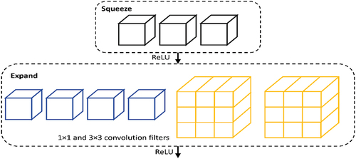
SqueezeNet consists of the fire module (Figure 7) that reduces parameters of the network by replacing 3 × 3 filters with 1 × 1 filters and hence reducing the number of input channels to 3 × 3 filters. It places downsampling late in the network so that convolution layers contain larger activation maps. Furthermore, the volume of the model is also scaled by deep compression. In comparison to AlexNet, SqueezeNet decreases the number of parameters by nearly 50 times while guaranteeing that there is no loss in accuracy and further the model volume is compressed to about 510 times the original volume (Iandola et al. 2016).

Figure 7. Fire protection module in SqueezeNet architecture.

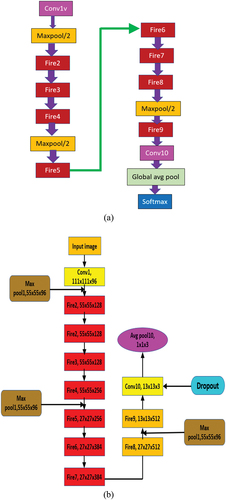
A schematic depiction and the overall network architecture of SqueezeNet is shown in Figure 8 (a) and (b), respectively.

Figure 8. (a) Schematic and (b) overall architecture of SqueezeNet model.

5.2. ResNet-50

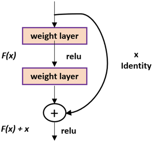
The other DNN model used in this manuscript is ResNet-50, which was proposed by Kaiming He et al. (He et al. 2016). Because of its ‘simplicity and practicality’, many methods have been built on the basis of ResNet-50. ResNet has been used in areas such as detection, segmentation and identification (He et al. 2016). The most important issue impacting the training of deep/large neural networks is the term ‘numerical stability’ of the network’s parameters. This issue is known as the exploding/vanishing gradient issue. ResNet, inherently due to its architectural design, stops all these issues from occurring in the network by skipping connections. The skip connections do not allow a vanishing/exploding gradient as they behave as gradients, allowing them to flow without being changed by a larger magnitude. In terms of applying it to the present network, it is the introduction of a simple addition of the identity function to the output as shown in Figure 9. In terms of architecture, if any layer ends up damaging the performance of the model in a plain network, it gets skipped due to the presence of the skip connections as shown in Figure 9.

Figure 9. Residual learning–building block.

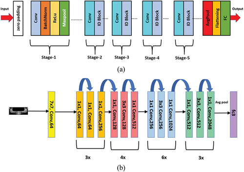
The schematic depiction and the overall network architecture of ResNet-50 consisting of 50 layers of DNN is shown in Figure 10 (a) and (b), respectively.

Figure 10. (a) Schematic representation and (b) overall architecture of ResNet-50 model.

5.3. EfficientNet-b0

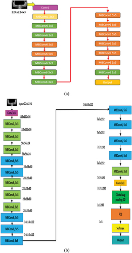
The other pretrained neural network that has been implemented for image classification is EfficientNet-b0. EfficientNet-b0 is the base model of this group that takes 224 × 224 pixels images as the input (Tan and Le 2019). This EfficientNet-b0 architecture implements mobile inverted bottleneck convolution (MBConv), which is very similar to MobileNetV2, although it is little large because of higher floating-point operation per second (FLOPS) budget. Generally, the models based on EfficientNet are known for their higher efficiency and accuracy over existing state-of-the-art CNN models, decreasing parameter size and FLOPS by their order of magnitude. While other CNN models employ ReLU that acts as an activation function, EfficientNet models use Swish that is a product of a sigmoid and linear activation function. Furthermore, EfficientNet-B0 deploys the inverted residual block that reduces the trainable parameters by a large number (Hridoy et al. 2021). The EfficientNet-b0 architecture is shown in Figure 11.

Figure 11. (a) Schematic representation and (b) overall architecture of EfficientNet-b0 model (He et al. 2016).

6. Materials and methods

6.1. Datasets

The dental image data (X-ray), comprising anonymised and unidentified panoramic dental X-ray images of 116 patients, have been obtained from the Noor Medical Center, Iran. The dental images contain various dental conditions from healthy/ideal edentulous, partially damaged edentulous (require bridges) and completely damaged edentulous cases that require complete dental prosthesis. All these sets of different cases have been segmented by two dentists manually. The complete dataset can be obtained from the Kaggle website that is publicly accessible at https://www.kaggle.com/daverattan/dental-xrary-tfrecords. The details of layers in each deep learning model and the input and output image sizes, respectively, are summarised in Table 2.

Table 2. Size of input/output images in each model.

Network Type	No. of layers	Parameters in millions	Input Image Size	Output Image Size
SqueezeNet	18	1.24	227 × 227	801 × 826
ResNet-50	50	25.6	224 × 224	1920 × 926
EfficientNet-b0	82	5.3	224 × 224	1920 × 926

6.2. Proposed methodology

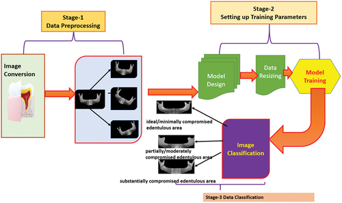
In this paper, dental X-ray images have been used for performing the multiclass classification of edentulous condition based on severity, which would require an appropriate clinical treatment (D’Souza Col and Dua 2011). The segmented dental images have been divided into three classes namely, ideal/minimally compromised edentulous area (no clinical treatment needed immediately), partially/moderately compromised edentulous area (require bridges, cast partial denture, resin bonded prosthesis, foundation restorations and fixed partial denture) and substantially compromised edentulous area (require complete denture prosthesis). In the initial phase of the proposed work, the image data are augmented and then pre-processed. Batch size determines both model generalisation and training time. A small batch size helps the model’s learning process from every individual example but results in longer training time. Small batch sizes are considered noisy, contributing to lower generalisation error and regularising effect. On the other hand, large batch size trains faster but model output does not capture the nuances in the data. As observed in Table 1, a common gap in the literature is that the effect of batch size on performance of deep learning models has not been investigated, which is attempted herein. In the current paper, the data are split into 70% training and 30% validation. In conclusion, the multiple output model is established for training the model. The data augmentation has been done by applying diverse types of processes such as translate, scale and rotate. Prior to the data augmentation, the dataset size was 82, and it has been increased to 160 after the augmentation process. The data augmentation has been done to grow the dataset size, which will produce more accurate and precise results. The process followed in the proposed methodology for multiclassification of dental X-Ray images using DNN is shown in Figure 12.

Figure 12. Multiclassification of dental X-ray images using SqueezeNet, ResNet-50 and EfficientNet-b0 DNN for patient clinical treatment.

The process of data augmentation followed in the present study is shown by a representative example in Figure 13. The parameters used for this purpose were: rotation between −90 ° and + 90°, translation by 10–35 pixels in X and Y directions and scaling between 1 and 2.

Figure 13. (a) Data augmentation by rotation (−90 to +90), (b) data augmentation by translate (shifting 10–35 pixels in X and Y direction) and (c) data augmentation by scaling from value of 1 to 2.

7. Results and discussion

The pretrained neural networks of SqueezeNet-18 layers, RestNet-50 and EffcientNet-b0 have been implemented with data augmentation using the Deep Network Designer module of Matlab 2022. Those networks used for classification include SqueezeNet, ResNet and EffcientNet-b0. The hyperparameters of the ANN networks such as learning rate = 0.0001 were kept constant for all networks for slower learning from the initial layers and then to proceed faster to the next layer. Epoch and validation frequency were kept as 25 and 5, respectively (optimised values) for all ANNs.

Furthermore, different batch size (3–6) and solver type-stochastic gradient descent with momentum (sgdm), root mean square propagation (rmsprop) and adaptive momentum estimation (adam) were implemented and tested for all types of neural networks (SqueezeNet, ResNet-50 and EffcientNet-b0 to optimise and achieve the highest possible accuracy in dental image classification based on the mandible condition of the patient (Amir Hossein Abdi et al. 2015). The comparison of the results of the various models have been plotted for augmented dataset that includes (Image rotation, translation and scaling) is shown in Figure 14. The comparison of network accuracy with and without data augmentation is shown in Figure 15.

Figure 14. Comparison of accuracy of SqueezeNet, ResNet-50 and EfficientNet-b0 DNNs for different solvers and batch size.

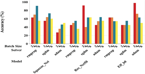
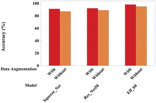
Figure 15. Comparison of max accuracy of each DNN model (with data augmentation) with its max accuracy achieved without data augmentation.

The confusion matrices obtained for the three best prediction models: SqueezeNet with rmsprop solver, batch size 5; ResNet-50 with sgdm solver, batch size 3; and EfficientNet-b0 with adam solver, batch size 3) are shown in Figures 16–18, respectively. The performance metrics give a better understanding of the predictions in comparison to the accuracy performance metrics. From the confusion matrices, the performance parameters such as Accuracy, Precision, Sensitivity (also called Recall), Specificity and F-1 score (Wijaya 0000; Yang et al. 2018; Sukegawa et al. 2020; Sivasundaram and Pandian 2021; Cejudo et al. 2021) have been calculated and listed in Table 3. To compare the relationship between true positive rate and false positive rate for each of the best accuracy models, their ROC curve is shown in Figure 19. EfficientNet-b0 is found to exhibit the highest true positive rate followed by SqueezeNet and ResNet-50. The difference between SqueezeNet and ResNet-50 is found to be quite small.

Figure 16. Confusion matrix for SqueezeNet (with data augmentation) with an accuracy of 91%.

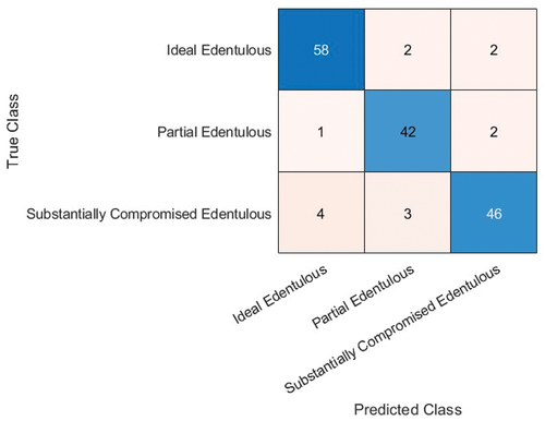
Figure 17. Confusion matrix for ResNet-50 (with data augmentation) with an accuracy of 92%.

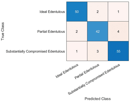
Figure 18. Confusion matrix for EfficientNet-b0 (with data augmentation) with an accuracy of 92%.

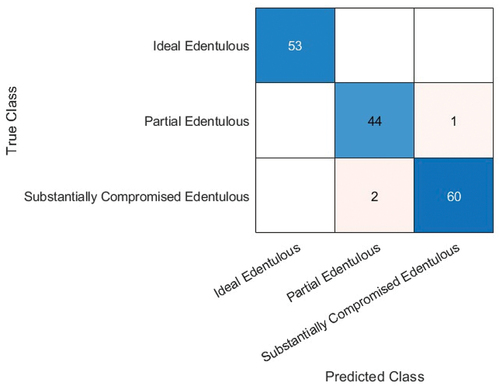
Figure 19. ROC curves for the best accuracy models obtained in the present study.

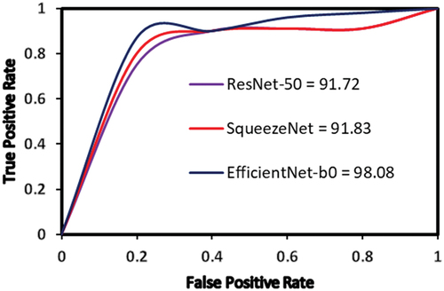
Table 3. Performance metrics of the best accuracy models.

Performance Metrics	SqueezeNet	ResNet-50	EfficientNet-b0
Accuracy (%)	91	92	98
Precision	0.9246	0.9178	0.98
Sensitivity	0.9122	0.9168	0.9818
Specificity	0.8257	0.8017	0.8329
F1-score	0.9183	0.9172	0.9808
Time duration	4 min, 30 s	4 min, 30 s	4 min, 30 s

A representative image dataset used for multiclassification of dental X-Ray images is shown in Figure 20. There are three stages of image processing done in this manuscript: stage-1 where image pre-processing for resizing occurs according to the desired input defined by the deep network type and data augmentation has been done with an increase in the size of dataset by rotating, scaling and Gaussian blur. Furthermore, the pre-processed image data are sent to stage-2 where appropriate model design is chosen along with data resizing for training and validation purposes (In all cases, the training and testing data have been kept as 70% and 30%). Also, in stage-2, the model is trained by optimising the hyperparameters such as learning rate, batch size and also different solvers. After model training, the image data are sent to stage-3 that consists of the classification layer, which predicts the output of the network type.

Figure 20. Sample image dataset containing segmented X-ray dental images for training DNN based on CNN for classification as ideal edentulous, partially damaged edentulous and completely damaged edentulous cases.

The highest validation accuracy of SqueezeNet was 91% (with data augmentation) highest for solver type – rmsprop and batch size 5 (refer Figure 21). This clearly establishes the optimised hyperparameters of SqueezeNet for the given dataset of dental images.

Figure 21. (a) Highest accuracy (with data augmentation) - SqueezeNet (b) and (c) highest accuracy (without data augmentation) - SqueezeNet.

It is imperative to note the type of solver and batch have a great impact on the validation and accuracy of the DNN as shown in Figure 14 which shows that the accuracy of SqueezeNet network by deploying sgdm and adam was only 73% (batch size − 5) and 50 % (batch size − 6), respectively (with data augmentation). Smaller batch helps good learning and accuracy of the training model but increases the training time, whereas large batch helps only in reduced learning and accuracy of the training model but reduces training time.

The highest validation accuracy of ResNet-50 was 92% (with data augmentation) for solver type-sgdm and batch size 5 (see Figure 22). This clearly establishes the optimised hyperparameters of ResNet-50 for the given dataset of dental images. It is imperative to note the type of solver and batch have a great impact on the validation and accuracy of the DNN as shown in Figure 14, which shows that the highest accuracy for ResNet-50 by deploying rmsprop and adam was only 55% (batch size-5) and 64% (batch size-5) (with data augmentation), respectively.

Figure 22. (a) Highest accuracy (with data augmentation) - ResNet-50 and (b) highest accuracy (without data augmentation) - ResNet-50.

The highest validation accuracy of EfficientNet-b0 was 98% for solver type-adam for batch size-3 (see Figure 23). This clearly establishes the optimised hyperparameters of EfficientNet-b0 for the given dataset of dental images. It is imperative to note that the type of solver and batch have a great impact on the validation and accuracy of the DNN as shown in Figure 14, which shows that the highest accuracy by deploying sgdm and rmsprop is 55% (batch size-5) and 46% (batch size-3), respectively, for the EfficientNet-b0.

Figure 23. (a) Highest accuracy (with data augmentation) - EfficientNet-b0 (b) and (c) highest accuracy (without data augmentation) - EfficientNet-b0.

It is most noted that the EfficientNet-b0 has outperformed SqueezeNet and ResNet-50 in terms of the overall highest validation accuracy. Also, it is imperative to note that the accuracy of Efficientb0 network (without data augmentation) with adam solver for a batch size of 3 is 95%, which is better than the highest validation accuracy of 91% for SqueezeNet (with data augmentation) and the highest validation accuracy of 92% of ResNet50 (with data augmentation).

The performance of the developed models is tested against a completely new panoramic radiographic image pertaining to a patient with partially edentulous mandible from Ahuja et al. (2019). The results obtained with the best accuracy models are shown in Figure 24. It is evident that the three models can accurately classify the type of edentulous condition.

Figure 24. Predictions of (a) SqueezeNet, (b) ResNet-50 and (c) EfficientNet-b0 against an image of a partially edentulous mandible (Ahuja et al. 2019).

8. Conclusions

The three pretrained DNNs (SqueezeNet, ResNet-50 and EfficientNet-b0) implemented using the Deep Network Designer module have been trained and validated for their accuracy in the classification of segmented dental images as ideal edentulous, partially compromised edentulous and substantially compromised edentulous cases, which is essential for improving the treatment quality and processing time of the patient, resulting in better health-care solutions. The comparative analysis of these pretrained neural networks (SqueezeNet, ResNet-50 and EfficientNet-b0) shows that EfficientNet-b0 outperformed other DNNs and achieved the highest accuracy of 98%. This is mainly due to compound scaling method that is inherently built within the EfficientNet-b0 (Tan and Le 2019). The compound scaling method augments the image recognition and classification as more input layers would be needed for larger input image and thus leads to broadening of the receptive field, resulting in a multilayer architecture essential to capture fine-grained patterns of a larger image (Lu et al. 2017). Our results are in agreement with Miglani and Bhatia (2021), who had implemented EffcientNet-b0, which resulted in 8.4 times parameter reduction and 16 times FLOPS reduction but performed better than ResNet-50.

Furthermore, these results indicate that the procedure can be implemented during the initial stage of clinical examination and analysis of dental images. The small dataset consisting of 116 patients has also contributed significantly to the success of this method. For future research, the multiclass classification of dental images could be done for larger datasets with more classes. Methodologies to implement a novel advanced DNN can be realised that can improve the performance of the existing network for image classification.

Nomenclature

${\beta }_1$ ${\beta }_2$	=	decay rates (gradient decay and squared gradient decay factors, respectively)
$\mathit{m}$	=	first moment vector
$\mathit{v}$	=	second moment vector
$\mathit{l}$	=	iteration number
$\mathit{\alpha }$ >0	=	learning rate
$\mathit{\theta }$	=	parameters vector
$\mathit{E}\left(\mathit{\theta }\right)$	=	loss function
$\mathit{\epsilon }$	=	constant added to avoid division by zero during optimisation
$E_R\left(\mathit{\theta }\right)$	=	loss function with regularisation
$\mathrm{\nabla E}\left(\mathit{\theta }\right)$	=	gradient of $\mathit{E}\left(\mathit{\theta }\right)$
$\mathit{w}$	=	weight factor
$\mathit{\lambda }$	=	regularisation factor (coefficient)
$\mathrm{\Omega }\left(\mathit{w}\right)$	=	regularisation function
$\mathit{\gamma }$	=	moment value used in SGDM algorithm

Acknowledgements

The authors would like to express their gratitude to the reviewer for the time taken to review the manuscript and their valuable comments/suggestions, which have undoubtably improved the quality of the manuscript. The authors express their hearty gratitude to the Manipal Institute of Technology, Manipal Academy of Higher Education, for providing the necessary infrastructural support to carry out this project.

Disclosure statement

No potential conflict of interest was reported by the author(s).

Additional information

Notes on contributors

G. Divya Deepak

Dr. G Divya Deepak is an Assistant Professor-Selection Grade in the Department of Mechanical and Industrial Engineering at Manipal Institute of Technology, India. He has done his Masters from University of Windsor, Canada. His Ph.D research work is in the field of atmospheric pressure cold plasma jets for biomedical applications (in collaboration with Central Electronics Engineering Research Institute,Pilani (CSIR-CEERI) Govt of India). His current research interests include the topics related to Dielectric barrier discharge based cold plasma jets, Application of Machine Learning/Deep Learning Techniques for Biomedical Image Processing and Advanced Manufacturing Methods.

Subraya Krishna Bhat

Dr. Subraya Krishna Bhat is an Assistant Professor in the Department of Mechanical and Industrial Engineering at Manipal Institute of Technology, India. He obtained his PhD in the area of Cardiovascular Biomechanics from Kyushu Institute of Technology, Japan being a recepient of the prestigious MEXT scholarship from the government of Japan for his doctoral reasearch. His current research interests include the topics related to Biomechanics/Continuum Mechanics, Application of Machine Learning/Deep Learning Techniques for Biomedical Data and Advanced Manufacturing Methods.

References

- Ahuja S, Jain V, Wicks R, Hollis W. 2019. Restoration of a partially edentulous patient with combination partial dentures. Br Dent J. 226(6):407–20. doi: 10.1038/s41415-019-0095-z.
- Al-Ghamdi ASA, Ragab M, Al-Ghamdi SA, Asseri AH, Mansour RF, Koundal D. 2022. Detection of dental diseases through X-ray images using neural search architecture network. Comput Intell Neurosci. 3500552:1–7. doi: 10.1155/2022/3500552.
- Amir Hossein Abdi DDS, Kasaei S, Mehdizadeh M. (18 November 2015). Automatic segmentation of mandible in panoramic x-ray. J Med Imag. 2(4):044003. 10.1117/1.JMI.2.4.044003
- Anand D, Arulselvi G, Balaji GN, Chandra GR. 2022. A deep convolutional extreme machine learning classification method to detect bone cancer from histopathological images. Int J Intell Sys Appl Eng. 10(4):39–47.
- Appe SN, Arulselvi G, Balaji GN. 2023. CAM-YOLO: tomato detection and classification based on improved YOLOv5 using combining attention mechanism. PeerJ Computer Science. 9:e1463.
- Bai YK. 2019. Target detection method of underwater moving image based on optical flow characteristics. J Coast Res. 93(sp1):668. doi: 10.2112/SI93-091.1.
- Bhalla K, Koundal D, Bhatia S, Khalid Imam Rahmani M, Tahir M. 2022. Fusion of infrared and visible images using fuzzy-based Siamese convolutional network. Comput Mater Continua. 70(3):5503. doi: 10.32604/cmc.2022.021125.
- Bhat SK, Deepak GD. 2023. Predictive modelling and optimization of double ring electrode based cold plasma using artificial neural network. Int J Eng. In Press.
- Bishop CM. 2006. Pattern recognition and machine learning. New York, NY: Springer.
- Bouchahma M, Ben Hammouda S, Kouki S, Alshemaili M and Samara K, “An Automatic dental decay treatment prediction using a deep convolutional neural network on X-Ray images,” 2019 IEEE/ACS 16th International Conference on Computer Systems and Applications (AICCSA), Abu Dhabi, United Arab Emirates, 2019, pp. 1–4, doi: 10.1109/AICCSA47632.2019.9035278.
- Cejudo JE, Chaurasia A, Feldberg B, Krois J, Schwendicke F. 2021. Classification of dental radiographs using deep learning. J Clin Med. 10(7):1496. doi: 10.3390/jcm10071496.
- Collobert R, Weston J, Bottou L, Karlen M, Kavukcuoglu K, Kuksa P. 2011. Natural language processing (almost) from scratch. J Mach Learn Res. 12:2493.
- D’Souza Col DSJ, Dua P. 2011. Rehabilitation strategies for partially edentulous - prosthodontic principles and current trends. Medical J Armed Forces India. 67(3):296. doi: 10.1016/S0377-1237(11)60068-3.
- Geetha V, Aprameya KS, Hinduja DM. 2020. Dental caries diagnosis in digital radiographs using back-propagation neural network. Health Inf Sci Syst. 8(8). doi: 10.1007/s13755-019-0096-y.
- Girshick R, Donahue J, Darrell T, et al. (2014). Rich feature hierarchies for accurate object detection and semantic segmentation. In Proceedings of the 2014 IEEE Conference on Computer Vision and Pattern Recognition (pp. 580–587). Washington, DC: IEEE Computer Society.
- Guo ZM, Jiang Y, Bi SH. 2018. Detection probability for moving ground target of normal distribution using an imaging satellite. Chin J Electron. 27(6):1309. doi: 10.1049/cje.2018.08.005.
- He K, Zhang X, Ren S, Sun J. (2016). Deep residual learning for image recognition. In 2016 IEEE Conference on Computer Vision and Pattern Recognition (CVPR); Jun 27–30; Las Vegas, NV, USA. IEEE. p. 770–778. doi: 10.1109/CVPR.2016.90.
- He K, Zhang X, Ren S, & Sun J. (2016). Deep residual learning for image recognition. In 2016 IEEE Conference on Computer Vision and Pattern Recognition.
- Hridoy RH, Akter F, Mahfuzullah M, & Ferdowsy F (2021). A computer vision-based food recognition approach for controlling. In 2021 International Conference on Information Technology (ICIT); Jul 14–15; Amman, Jordan; IEEE. p. 543–548. doi:10.1109/ICIT52682.2021.9491783.
- Iandola FN, Han S, Moskewicz MW, Ashraf K, Dally WJ, Keutzer K. 2016 . SqueezeNet: AlexNet-level accuracy with 50x fewer parameters and <0.5 MB model size. arXiv, arXiv: 1602.07360. https://arxiv.org/abs/1602.07360v4.
- Ilić I, Vodanović M and Subašić M, “Gender estimation from panoramic dental X-ray images using deep convolutional networks,” IEEE EUROCON 2019 -18th International Conference on Smart Technologies, Novi Sad, Serbia, 2019, pp. 1–5, doi: 10.1109/EUROCON.2019.8861726.
- Imangaliyev S, van der Veen MH, Volgenant CMC, Keijser BJF, Crielaard W, Levin E. 2016. Deep learning for classification of dental plaque images. In: Pardalos P, Conca P, Giuffrida G Nicosia G, editors. Machine learning, optimization, and big data. MOD 2016. Lecture notes in computer science(). Vol. 10122. Cham: Springer. doi:10.1007/978-3-319-51469-7_34.
- Jusman Y, Anam MK, Puspita S, Saleh E, Kanafiah SNAM and Tamarena RI, “Comparison of dental caries level images classification performance using KNN and SVM methods,” 2021 IEEE International Conference on Signal and Image Processing Applications (ICSIPA), Kuala Terengganu, Malaysia, 2021, pp. 167–172, doi: 10.1109/ICSIPA52582.2021.9576774.
- Kingma D, & Ba J (2014). Adam: a method for stochastic optimization. arXiv preprint arXiv:1412.6980.
- Krois J, Ekert T, Meinhold L, Golla T, Kharbot B, Wittemeier A, Dörfer C, Schwendicke F. 2019. Deep learning for the radiographic detection of periodontal bone loss. Sci Rep. 9(1):8495. doi: 10.1038/s41598-019-44839-3.
- Laishram A and Thongam K, “Detection and classification of dental pathologies using Faster-RCNN in orthopantomogram radiography image,” 2020 7th International Conference on Signal Processing and Integrated Networks (SPIN), Noida, India, 2020, pp. 423–428, doi: 10.1109/SPIN48934.2020.9071242.
- Lee J-H, Kim D-H, Jeong S-N, Choi S-H. Detection and diagnosis of dental caries using a deep learning-based convolutional neural network algorithm. J Dent. 2018. 77:106–111. doi: 10.1016/j.jdent.2018.07.015.
- Leonard JK. 2019. Image classification and object detection algorithm based on convolutional neural network. Sci Insigt. 31(1):85. doi: 10.15354/si.19.re117.
- Liu L, Xu J, Huan Y, Zou Z, Yeh SCC, Zheng L-R. 2020. A smart dental Health-IoT platform based on intelligent hardware, deep learning, and mobile terminal. IEEE J Biomed Health Informat. 24(3):898–906. March. doi:10.1109/JBHI.2019.2919916
- Long J, Shelhamer E, & Darrell T (2015). Fully convolutional networks for semantic segmentation. In Proceedings of the 2015 IEEE Conference on Computer Vision and Pattern Recognition; Jun 7–12; Boston, MA, USA.
- Lu Z, Pu H, Wang F, Hu Z, Wang L. 2017. The expressive power of neural networks: a view from the width. 31st Conference on Neural Information Processing Systems (NIPS 2017); Dec 4–9; Long Beach, CA, USA. https://arxiv.org/abs/1709.02540v3
- Ma LY, Liu XW, Zhang Y, Jia SL. 2022. Visual target detection for energy consumption optimization of unmanned surface vehicle. Ener Rep. 8:363. doi: 10.1016/j.egyr.2022.01.204.
- Masic F. 2012. Information systems in dentistry. Acta Inform Med. 20(1):47–55. doi: 10.5455/aim.2012.20.47-55.
- McGarry TJ, Nimmo A, Skiba JF, Ahlstrom RH, Smith CR, Koumjian JH. 1999. Classification System for complete edentulism. J Prosthodontics. 8(1):27. doi: 10.1111/j.1532-849X.1999.tb00005.x.
- Miglani V, Bhatia M. 2021. Skin lesion classification: a transfer learning approach using EfficientNets. In: Hassanien A, Bhatnagar R, and Darwish A, editors. Advanced machine learning technologies and applications. AMLTA 2020. Vol. 1141. Springer, Singapore: Springer. doi: 10.1007/978-981-15-3383-9_29.
- Moutselos K, Berdouses E, Oulis C and Maglogiannis I, “Recognizing occlusal caries in dental intraoral images using deep learning,” 2019 41st Annual International Conference of the IEEE Engineering in Medicine and Biology Society (EMBC), Berlin, Germany, 2019, pp. 1617–1620, doi: 10.1109/EMBC.2019.8856553.
- Nair R, Alhudhaif A, Koundal D, Doewes RI, Sharma P. 2021. Deep learning-based COVID-19 detection system using pulmonary CT scans. Turk J Electr Eng Co. 29(SI–1):2716–2727. doi:10.3906/elk-2105-243.
- Oquab M, Bottou L, Laptev I, et al. (2014). Learning and transferring mid-level image representations using convolutional neural networks. In Proceedings of the 2014 IEEE Conference on Computer Vision and Pattern Recognition (pp. 1717). Washington, DC: IEEE Computer Society.
- Prajapati SA, Nagaraj R and Mitra S, “Classification of dental diseases using CNN and transfer learning,” 2017 5th International Symposium on Computational and Business Intelligence (ISCBI), Dubai, United Arab Emirates, 2017, pp. 70–74, doi: 10.1109/ISCBI.2017.8053547.
- Rad AE, Rahim MSM, Rehman A, Saba T. 2016. Digital dental X-ray database for caries screening. 3D Res. 7(2). doi: 10.1007/s13319-016-0096-5.
- Rana A, Yauney G, Wong LC, Gupta O, Muftu A and Shah P, “Automated segmentation of gingival diseases from oral images,” 2017 IEEE Healthcare Innovations and Point of Care Technologies (HI-POCT), Bethesda, MD, USA, 2017, pp. 144–147, doi: 10.1109/HIC.2017.8227605.
- Rathod J, Waghmode V, Sodha A, & Bhavathankar P (2018). Diagnosis of skin diseases using convolutional neural networks. In 2018 Second International Conference on Electronics, Communication and Aerospace Technology (ICECA) (pp. 1048–1051). Coimbatore, India. doi: 10.1109/ICECA.2018.8474593.
- Salunke D, Mane D, Joshi R, Peddi P. Customized convolutional neural network to detect dental caries from radiovisiography (RVG) images. Int J Advan Tech & Eng Exp. 2022. 9:91. doi: 10.19101/IJATEE.2021.874862.
- Shah N. 2014. Recent advances in imaging technologies in dentistry. World J Radiol. 6(10):794. doi: 10.4329/wjr.v6.i10.794.
- Simonyan K, Zisserman A. 2015. Very deep convolutional networks for large-scale image recognition. arXiv. https://arxiv.org/abs/1409.1556v6.
- Singh P, Kaur R. 2020. An integrated fog and artificial intelligence smart health framework to predict and prevent COVID-19. Global Trans. 2:283. doi: 10.1016/j.glt.2020.11.002.
- Singh P, Kaur R. 2021. Implementation of the QoS framework using fog computing to predict COVID-19 disease at an early stage. World Journal Of Engineering. 19(1):80. doi: 10.1108/WJE-12-2020-0636.
- Sivasundaram S, Pandian C. 2021. Performance analysis of classification and segmentation of cysts in panoramic dental images using convolutional neural network architecture. Int J Imaging Syst Technol. 31(4):2214–2225. doi: 10.1002/ima.22625.
- Sukegawa S, Yoshii K, Hara T, Yamashita K, Nakano K, Yamamoto N, Nagatsuka H, Furuki Y. 2020. Deep neural networks for dental implant system classification. Biomolecules. 10(7):984. doi: 10.3390/biom10070984.
- Szegedy C, Liu W, Jia Y, et al. (2015). Going deeper with convolutions. In Proceedings of the 2015 IEEE Conference on Computer Vision and Pattern Recognition (pp. 1). Washington, DC: IEEE Computer Society.
- Tan M, & Le Q (2019). EfficientNet: rethinking model scaling for convolutional neural networks. arXiv, arXiv:1905.11946.
- Tan M, Le QV. 2019. EfficientNet: rethinking model scaling for convolutional neural networks”, The 36th International Conference on Machine Learning; Jun 9-15; Long Beach, California, USA.
- Tian S, Dai N, Zhang B, Yuan F, Yu Q and Cheng X, “Automatic classification and segmentation of teeth on 3D dental model using hierarchical deep learning networks,” in IEEE Access, vol. 7, pp. 84817–84828, 2019, doi: 10.1109/ACCESS.2019.2924262.
- Wijaya E, “Implementation analysis of GLCM and naive Bayes methods in conducting extractions on dental image,” International Conference on Informatics, Engineering, Science and Technology (INCITEST) 9 May 2018, 407, 012146, DOI 10.1088/1757-899X/407/1/012146.
- Wu WZ, Zou JW, Chen J, Xu SY, Chen ZP. 2021. False-target recognition against interrupted-sampling repeater jamming based on integration decomposition. IEEE Trans Aerosp Electron Syst. 57(5):2979. doi: 10.1109/TAES.2021.3068443.
- Yang J, Xie Y, Liu L, Xia B, Cao Z and Guo C, “Automated dental image analysis by deep learning on small dataset,” 2018 IEEE 42nd Annual Computer Software and Applications Conference (COMPSAC), Tokyo, Japan, 2018, pp. 492–497, doi: 10.1109/COMPSAC.2018.00076.
- You W, Hao A, Li S, Wang Y, Xia B. 2020. Deep learning-based dental plaque detection on primary teeth: a comparison with clinical assessments. BMC Oral Health. 20(1):141. doi: 10.1186/s12903-020-01114-6.