A CNN-based strategy to automate contour detection of the hip and proximal femur using DXA hip images from longitudinal databases (CLSA and CaMos)

ABSTRACT

Hip fractures contribute significantly to mortality in older adults. New methods to identify those at risk use dual-energy X-ray absorptiometry (DXA) images and advanced image processing. However, DXA images have an overlapping femur and pelvis and may contain boundary lines, making automation challenging. Herein, a 5-layer U-net convolutional neural network (CNN) was developed to segment the femur from hip DXA images. Images were used from the Canadian Longitudinal Study on Aging (CLSA, N=104) and Canadian Multicentre Osteoporosis Study (CaMos, N=105) databases for training, with manual contour drawing defining the ‘true output’ of each image. An algorithm was then developed to mask each hip image, and trained to predict subsequent masks. The CNN was tested with 44 additional CLSA images and 42 CaMos images. This proposed approach had an accuracy and intersection over union (IoU) of 97% and 0.57, and 93% and 0.51, for CaMos and CLSA scans, respectively. Furthermore, a series of augmentation techniques was applied to increase the data size, with accuracies of 96% and 94%, and IoU of 0.53 and 0.50. Overall, our strategy automatically determined the contour of the proximal femur using various clinical DXA images, a key step to automate fracture risk assessment in clinical practice.    

KEYWORDS:

• Canadian Longitudinal Study on Aging (CLSA)
• image segmentation
• machine learning
• hip fracture
• dual-energy X-ray absorptiometry (DXA)

Introduction

Osteoporosis is a disease commonly associated with age that reduces bone mass and strength (Raisz 2005). Hip fractures are one of the leading causes of mortality in older adults (Abrahamsen et al. 2009). As such, identifying people at risk is crucial for clinicians to prevent fracture such that individualised interventions (e.g., pharmaceutical, mechanical) can be applied. Currently, osteoporosis (and corresponding hip fracture risk) is diagnosed based on T-score calculated from dual-energy X-ray absorptiometry (DXA) scans; however, this has been shown to be poorly correlated with actual fracture risk (Cranney et al. 2007).

New advances in technology offer the opportunity for greater diagnostic accuracy and ultimately better patient outcomes. One previously-developed fracture risk algorithm (Jazinizadeh and Quenneville 2020) uses a technique called statistical shape and appearance modelling (SSAM) to characterise the shape and distribution of mineral through the proximal femur, thus extracting more information from each clinical DXA scan than simply a single bone mineral density (BMD) measure. This technology uses logistic regression to improve the prediction of fracture risk and has shown substantial improvement over the clinical standard of T-score (Jazinizadeh et al. 2020).

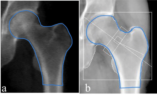
This SSAM technique requires the manual application of landmarks to each image. In order to improve the overall accuracy of the SSAM algorithm, more data must be used in the training set. Hence, in order to expand the SSAM algorithm to larger longitudinal databases such as Canadian Multicentre Osteoporosis Study (CaMos; ~9400 baseline and follow-up DXA scans) and the Canadian Longitudinal Study on Aging (CLSA; ~50,000 baseline and follow-up DXA scans) (Raina et al. 2009) a technique must be developed to automatically detect the contour of the hip and proximal femur. This is also a crucial step towards clinical implementation where manual landmarking is impractical. Therefore, it is important to develop an automated algorithm that accepts all types of clinical hip DXA images and extracts these contours. The main difference between hip DXA images from the CLSA and CaMos is that CLSA includes white boundary lines along the femur (Figure 1a), and CaMos does not (Figure 1b). In both databases, each DXA image comprised of both the pelvis and femur. Two primary challenges exist with automatically extracting the contour of the hip and proximal femur using pre-existing methods. These are 1) the overlap between the pelvis and femoral head and 2) the white boundary lines along the femur in some images. Therefore, other methods such as pixel thresholding and pre-built object detection algorithms were tested and not successful due to the complexity of the DXA image.

Figure 1. Standard clinical hip DXA images. (a) hip DXA image from the CLSA, with the white boundary lines (b) hip DXA image from the CaMos, with no white boundary lines.

The DXA images provided from the CaMos are clinical hip images; however, these images do not contain white boundary lines along the femur or anywhere on the image. However, hip DXA images provided from the CLSA contain white boundary lines, which are primarily used for clinical assessments. Adding and removing the lines are options technicians can adjust on the DXA software (e.g., Hologic’s APEX System Software). The default hip DXA image is usually set with the white lines on the image. Hence, longitudinal databases such as CLSA keep the standard default hip DXA image, while in CaMos hip DXA scans they were removed before exporting.

A convolutional neural network (CNN) is a technique that is widely used for object detection and image segmentation. More specifically, a U-net architecture has been found to be an effective approach for biomedical segmentation applications, achieving high accuracy when used for various biomedical applications (Ronneberger 2017). Furthermore, U-net has been immensely applied to medical imaging segmentation and has previously been widely used due to its accuracy (Lu et al. 2022; Yin et al. 2022). Deep neural networks have been developed to automate femur segmentation from Computed Tomography (CT) and magnetic resonance (MR) images, with high accuracy and efficiency (Deniz et al. 2018; Bjornsson et al. 2021). Based on the high dice similarity scores in these previous studies, CNN is considered to have great potential to be used for management of osteoporosis and fracture risk. The purpose of our study was to propose a technique to automate the detection of the hip and proximal femur’s contour for DXA scans with an overlapping femur and pelvis, and the potential presence of boundary lines. This will allow researchers and medical practitioners to automatically determine the contour of the hip and proximal femur using all types of clinical DXA images, constituting a key step forward towards a clinical implementation of a fully automated fracture risk assessment tool.

Methods

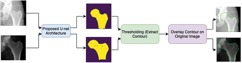
Images were obtained from CLSA and CaMos (Figure 1). Due to the complexity of the images, a 2-dimensional (2D) CNN was designed to accept both types of standard clinical images and extract the hip and proximal femur’s contour (Figure 2). This model was built entirely using Python TensorFlow v2, using the Keras API (application programming interface) on Google Colaboratory (Colab). Google Colab provides free of charge access to computer resources such as Graphics Processing Units (GPU) and Tensor Processing Units (TPU) (Bisong 2019). A U-net architecture was used.

Figure 2. Proposed CNN strategy to automatically detect the contour. First, the input images are applied to the proposed U-net architecture, which will output the predicted masks of each image. Then by applying thresholding, the contour is extracted and is then overlayed on the original input image.

Pre-processing & data preparation

Due to the availability of time and DXA scans, both the CLSA data and CaMos data were divided to have 70% of the data in the training set (104 and 105 images, respectively). To allow a supervised approach to be used, every input image had an associated ‘true output’ image that was created by manually drawing the correct contour along the edge of the femur (Figure 3a,b), which was performed by the same author.

Figure 3. (a) corresponding ‘true output’ of the input image (Figure 1a) and (b) corresponding ‘true output’ of the input image (Figure 1b).

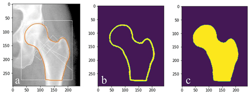
A mask generator was also developed where each true output image (Figure 4a) was inputted, and a binary mask was created based on pixel intensities (Figure 4b). A pixel intensity value corresponding to the manual line was used to binarize the image, where the femur was subsequently filled (Figure 4c).

Figure 4. (a) the ‘true output’ image manually drawn. (b) the image was binarized based on the pixel intensity. (c) the binary outline was subsequently filled to represent the region of the hip and proximal femur.

Contour detection of the femur and U-net model

The U-net model consisted of two main paths, the contracting (downsampling) path and the expanding (upsampling) path. These are respectively known as the encoder and decoder, which encapsulates a five-layer model (Figure 5). The input image was downsampled in the contracting path, which increased the number of channels. This allowed for the extraction of more complex features; in this case this model had three main channels with an input image size of 160 × 160 pixels.

Figure 5. Proposed U-net architecture. (a) contracting path, (b) expanding path.

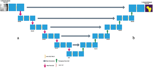
The encoder was built using MobileNetV2, which comprised of depthwise convolution to separate features, linear bottlenecks between layers and shortcut connections between bottlenecks (Sandler et al., 2018). Using MobileNetV2 allows for image segmentation, classification and object recognition while maintaining low computational time and high efficiency. Although there are other existing pretrained models that achieve superior results, MobileNetV2 was chosen due to its simpler architecture, lower complexity, faster computation, and needing minimal computation resources, in comparison to others (e.g., ResNet (Sunnetci et al. 2022)). The MobileNetV2 applied a deep convolution filter with a 1 × 1 pixel resolution followed by a 3 × 3 depthwise separable convolution filter and then a 1 × 1 convolution (Sandler et al., 2018; Toğaçar et al. 2021). When convolving the image with a 3 × 3 filter, this causes the image to get smaller. As such, at the end of each layer zero padding was done to preserve the original size of the input. In addition, this model used both batch normalisation and ReLU6 activation function. In MobileNetV2, batch normalisation is added behind every convolutional layer that is done.

In the decoder path, Pix2Pix upsampling was used. This required an inverse operation of the pooling layer known as a transposed convolution layer. By upsampling the input, this technique learned the complete details of the image. Every step learned the mapping from the input image to output image. The skip connections were also used to pass features from the downsampling path to the upsampling path in order to retrieve spatial information that was lost during downsampling (Bjornsson et al. 2021).

The dataset was split into four batches; therefore, each batch had 25 and 26 images for CaMos and CLSA datasets, respectively. For the CLSA images the model was trained and validated using 170 epochs; for the CaMos 150 epochs were used (determined based on the maximum before overfitting, defined as the training loss value reaching zero). The epoch sizes were selected by training the model through a series of epochs from zero to 200. The loss and accuracy were examined to determine the optimal epoch size that minimised error while increasing the accuracy. Overfitting is a common problem with training the model with too many epochs, hence epochs sizes over 170 and 150, for CLSA and CaMos, respectively were not chosen. Overfitting was avoided by ensuring that the accuracy did not fully saturate to 100% while keeping the loss low, the more epochs the model runs the longer the model is trained. The U-net model for both CLSA and CaMos images was evaluated using the Sparse Categorical Cross-entropy loss function and the Adam optimiser with a learning rate of 1 × 10⁻⁴ to test the overall performance of the model.

The CNN was evaluated for each image type using 30% of the data for testing from CLSA and CaMos (44 and 42 images, respectively) (testing data for both databases were not included in the training data). Dataset splits of 70:30 for both CLSA and CaMos were used as this ratio is commonly adopted in CNN models (El Saleh et al. 2019). The ‘true output’ was defined based on manual identification, as in the training set, and was then compared to the predicted output from the model. Both the input images and the mask were used to determine the predicted output, thus assessing the overall accuracy of the model. The accuracy metric that was used in Keras was Sparse Categorical Accuracy, which was calculated based on the percentage of predicted values (output) that match with the actual ‘true output’ pixel value labels. Furthermore, intersection over union (IoU) was measured, which reports the overlap between two bounding boxes (true output and predicted output) on a scale from 0 to 1 (where 1 indicates a perfect overlap between the two boxes and 0 indicates no overlap between the boxes).

The final contour output used the predicted mask and applied a technique called thresholding (Ma et al. 2010), which was used to determine the edge of the hip and proximal femur (i.e., the contour) by examining the nearby pixels along the object. Finally, the extracted contour was overlayed on top of the original input image.

Data augmentation

The most common solution for having limited data to build and train machine learning models is data augmentation. Due to limited availability of data, augmentation of both data sets (CLSA and CaMos) was applied. A series of augmentation techniques were applied to the images of both training sets, which were 1) flipping the images vertically, 2) sharpening each image by randomly varying the value between zero (no sharpening) and one (full sharpening), and 3) rotating the image by −45 to 45 degrees. In addition, Gaussian noise was added within a maximum of 10% of the maximum pixel value. Gaussian noise is noise sampled using a Gaussian distribution with a mean of zero and standard deviation of the value of the ‘added Gaussian noise’. The final augmentation technique that was applied was resizing, which scaled the image from 50% to 150%. For both datasets separately, these techniques were applied to their respective training sets and augmented 5-fold the original amount, referred to as offline augmentation. This technique is when the final dataset size changes by a factor equal to the number of augmentation techniques applied (Shorten & Khoshgoftaar, 2019). The CLSA and CaMos models were trained and validated using 170 epochs and 150 epochs, respectively. The resulting augmented model was then evaluated using the same testing as previously described.

Results

U-Net CNN model

CaMos (No white boundary lines)

This model was trained and validated using 150 epochs. The loss and accuracy for the training data were 2.89 × 10⁻⁴ and 0.99 (i.e., 99%), respectively (Figure 6a). For the validation data, the loss and accuracy of this model were 0.0029 and 0.99 (i.e., 99%), respectively (Figure 6b). The training and validation sets had a mean IoU of 0.61 and 0.60, respectively (Table 1). The total training time was 342.9 s, where the first epoch took 30 s and each subsequent epoch was 2.1 s.

Figure 6. For the CaMos dataset, a) the loss of the training data over the span of 150 epochs. b) the loss of the validation data over 150 epochs.

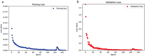
Table 1. Summary of U-net output.

Database	Training				Testing
	Training Accuracy	Training Loss	IoU	Training Time (s)	Testing Accuracy	Testing Loss	IoU	Execution Time (s)
CLSA	0.99 (99%)	0.000489	0.61	368	0.93 (93%)	0.50	0.51	1.01
CaMos	0.99 (99%)	0.000289	0.56	343	0.97 (97%)	0.27	0.57	1.03

After testing the CaMos data, the model was able to predict the masks of each testing image (N = 42) with a loss and accuracy of 0.27 and 0.97 (i.e., 97%), respectively. In addition, the testing data produced a mean IoU of 0.57 (Table 1). The overall execution time was 1.03 s.

CLSA (white boundary lines)

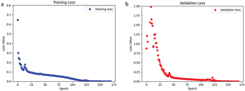
After training and validating this model using 170 epochs, the loss and accuracy for the training data were 4.89 × 10⁻⁴ and 0.99 (i.e., 99%), respectively (Figure 7a). Also, the loss and accuracy for the validation data was 6.62 × 10⁻⁴ and 0.99 (i.e., 99%), respectively (Figure 7b). Loss values decreased substantially over the first 35 of the 170 trained epochs. The training and validation sets had a mean IoU of 0.56 and 0.54, respectively (Table 1). The total training time was 368 s, where the first epoch took 30 s and each subsequent epoch was 2 s.

Figure 7. For the CLSA dataset, a) the loss of the training data over the span of 170 epochs. b) the loss of the validation data over 170 epochs.

After testing the CLSA data, the model was able to predict the masks of each testing image (N = 44) with an accuracy of 0.93 (i.e., 93%) and a loss of 0.50. In addition, the testing data produced a mean IoU of 0.51 (Table 1). The overall execution time for testing the CLSA images was 1.01 s.

Data augmentation

After training and validating the CLSA model using 170 epochs, the loss and accuracy for the training data were 0.1014 and 0.95 (i.e., 95%), respectively. In addition, the loss and accuracy for the validation data were 0.1233 and 0.94 (i.e., 94%), respectively (Table 2). Similarly, CaMos was trained and validated using 150 epochs, and the loss and accuracy for the training data were 0.002 and 0.99 (i.e., 99%), respectively. Also, the loss and accuracy for the validation data were 0.05 and 0.98 (i.e., 98%), respectively (Table 2). The training and validation loss for both CLSA and CaMos show a downward trend as more epochs were trained (Figure 8).

Figure 8. For the CaMos augmented dataset, a) the loss of the training data over the span of 150 epochs. b) the loss of the validation data over 150 epochs. For the CLSA augmented dataset, c) the loss of the training data over the span of 170 epochs. d) the loss of the validation data over 170 epochs.

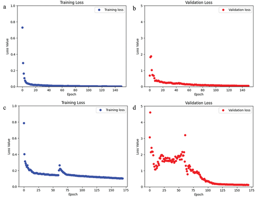
Table 2. Summary of U-net output with the augmented data.

Database	Training				Testing
	Training Accuracy	Training Loss	IoU	Training Time (s)	Testing Accuracy	Testing Loss	IoU	Execution Time (s)
CLSA	0.95 (95%)	0.1014	0.53	1088	0.94 (94%)	0.3262	0.50	1.01
CaMos	0.99 (99%)	0.0020	0.58	906	0.96 (96%)	0.2572	0.53	1.01

For the augmented CLSA data, the training and validation data had a mean IoU of 0.53 and 0.52, respectively (Table 2). The testing data produced a mean IoU of 0.50. In addition, the augmented CaMos data, had a mean IoU of 0.58 and 0.55 for the training and validation datasets, respectively.

Final output: contour of the femur

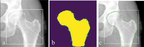
For each test set the contour was extracted and overlayed on the original image for the CaMos database (Figure 9), and CLSA database (Figure 10).

Figure 9. a) CaMos hip DXA scan from testing set. b) the corresponding predicted output mask from the model. c) the contour projected on to the original input image.

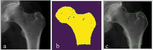
Figure 10. a) CLSA hip DXA scan from testing set. b) the corresponding predicted output mask from the model. c) the contour projected on to the original input image.

Discussion

In this work, a U-net CNN model was developed to automate the segmentation of DXA hip images in order to extract the contour of the hip and proximal femur. This was successfully demonstrated on standard clinical DXA images, addressing both the overlap with the pelvis and the possible presence of white boundary lines. This approach is a critical step towards automating femur contour identification for widespread implementation of enhanced fracture risk prediction algorithms.

The CNN was trained and tested using two different image sets from the CLSA and CaMos. The main challenges of these datasets were with the overlapping of the pelvis and femur, as well as the white boundary lines present on the hip DXA images. Using the CaMos (without white boundary lines) images, the model achieved a 97% accuracy on the testing data. Similarly, using CLSA (with white boundary lines) images achieved a 93% accuracy on the testing data. At a glance, these results demonstrate the effectiveness of this CNN strategy. However, there is a 3% and 7% loss from CaMos and CLSA, respectively that the contour may not have been accurately identified. The clinical importance of how ‘good’ 97% versus 93% has not been quantified. This aspect is beyond the scope of this study; however, future work should investigate how effective the CNN strategy is and determine how well both databases perform by applying the predicted contours to the SSAM fracture risk algorithm. This will determine if automatic detection of the hip and proximal femur’s contour using this CNN strategy is adequate, or whether these small errors are important enough that they would affect a clinical assessment of fracture risk.

The model achieved an IoU of 0.57 and 0.51 on the testing data for both CaMos and CLSA databases. This demonstrates that the intersection between the ‘true output’ and the predicted output was more than 50%. Even though theoretically IoU of 1.0 is a 100% overlap, this is often considered impossible to achieve, where similar previous work on training a deep learning model for classifying bone tumours on radiographs achieved a mean IoU of 0.52, which allowed for a successful model that automatically detected the location of the tumour (von Schacky et al. 2021). Similar results have been reported in another previous CNN segmentation study, which achieved a high accuracy of 0.92 and 0.93 and a mean IoU of 0.59 and 0.44, for the testing data of two different objects that were segmented (Majeed et al. 2018).

CLSA and CaMos are large longitudinal databases that encapsulate over 50,000 DXA images combined; however, in the present study only approximately 100 images from each dataset were used to train the CNN. This was due to the laborious work needed to prepare the images for the CNN (i.e., manually identifying the correct contour for testing the proposed strategy). However, very good results were still achieved in this study with the current data size used. This demonstrates the great potential of this developed CNN. Increasing the training set size would only improve our CNN to produce a more accurate contour detection algorithm.

Currently, the training and testing set sizes for both CLSA and CaMos were both 70:30 split. Ratios of 90:10, 80:20 and 70:30 have been successfully used with high accuracy (El Saleh et al. 2019). Hence, due to the limited overall data, and ensuring that the reliability and robustness is tested, 70:30 split was done to increase the size of the testing data.

For every input image that was used for training this model, a ‘true output’ was created to compare the predicted results. This method consisted of manually outlining the contour of the femur for every DXA image and creating a ‘true mask’ for every input that was used for training the CNN. This was done by the same author to ensure consistency among all images. One of the main challenges faced was successfully using different approaches for automatically detecting the contour of the femur. Different approaches were tested such as the Canny, Sobel method and thresholding, as these are extensively used for edge detection. However, the complexity of the hip DXA image did not allow these methods to produce an accurate result. Most medical images contain multiple layered anatomical features that contain non-uniform intensities and noise which result in failure of these basic algorithms (Ferreira et al. 2012). In medical image analysis and processing, various denoising techniques (Goceri 2023) and intensity normalisations have been used with different medical images (Goceri 2018). However, they may increase computational costs. Hence, a U-net CNN approach was developed to tackle this problem.

U-net architectures (such as was used in this present study) have been commonly used for image segmentation with high performance (Deniz et al. 2018; Peng et al. 2020; Bjornsson et al. 2021). A standard U-net contains a 5-layer structure in each path which allows us to solve more complicated image segmentation problems (Ronneberger et al. 2015). U-net structure can be modified to either greater or less than 5-layers for each path, and this is usually decided based on the type of application (Deniz et al. 2018; Peng et al. 2020; Bjornsson et al. 2021). U-net architecture has many advantages for segmentation process, such as the encoder and decoder structure allowing the model to capture small and large features within the image. Another main advantage of U-net for image segmentation is the fewer training samples required; U-net has shown to produce good results while using limited training data (Du et al. 2020). This can be done because of the features such as skip connections that help generate information and map it from the encoder to decoder to avoid the loss of information. Finally, another main advantage to U-net is the ability to easily adapt U-net models to other biomedical applications (Du et al. 2020).

Many researchers believe building a deep layered U-net structure allows for a more accurate output; however, when the image is in the expanding path some details are missed due to image loss from the contracting path. The design of the CNN structure is completely based on the task at hand and while developing the CNN, different pre-trained models can be used. However, CNN models can also be developed without using any pre-trained models. MobilenetV2 is a pre-trained model that contains more than a million images classified images (Sandler et al. 2018). This pre-trained model was used as the encoder for this model, as it assisted in classifying DXA images. MobilenetV2 has been previously used as an encoder for image segmentation (Peng et al. 2020; Kanadath et al. 2021). The benefits of using pre-trained models in CNN are achieving the most accurate results, faster computation, and better overall performance.

The optimiser and activation function should be chosen carefully. While there are various optimisers (e.g. Sobolev gradient-based (Goceri 2020a) and Lagrangian optimiser (Kervadec et al. 2022)) and activation functions (Kiseľák et al. 2020) implemented with deep networks to solve different classification problems, we applied the Adam and ReLU due to their efficiency in the proposed architecture with our datasets. The results herein were achieved using a Sparse Categorical cross entropy loss function with an Adam optimiser (lr = 1×10⁻⁴), which allowed for the model to learn at a slow rate, minimising the loss. These results are currently higher than other studies that have done image segmentation using a Sparse Categorical cross entropy loss function with an Adam optimiser, where accuracies on the order of 88% have been previously reported (Tawde et al. 2021). However, this present study produced similar results to another study, where the accuracy of the CNN was 97.4%, using a Sparse Categorical cross-entropy loss function with a N-Adam optimiser (Kakarla et al. 2021). This demonstrates the effectiveness of using these loss and accuracy functions, over the most commonly known metric (e.g., dice similarity coefficient) for image segmentation (Kakarla et al. 2021; Tawde et al. 2021). The Sparse Categorical Accuracy metric calculates the number of predictions that match the integer labels, which in this case is the pixel value. An advantage of this metric is that it calculates the mean accuracy over all the predictions and accounts for true negative predictions. In general, the metrics used in this present study were selected due to their robustness and accuracy for computing the loss for image segmentation.

Currently, there is very limited literature on applying image-based machine learning to either longitudinal database used herein (CLSA and CaMos). A recent study used the CLSA database and built a CNN model to identify vertebral fractures while being able to generalise between various DXA machine manufactures (Monchka et al. 2022). The CNN model achieved a sensitivity of over 90% while using the CLSA as well as other databases combined (Monchka et al. 2022). Although this application is different, the use of longitudinal databases such as CLSA and CaMos in machine learning models will tend to yield superior results due to their diverse images from various demographics, which allows improvement of the model.

It is known that deep networks are data-hungry, and several augmentations have been applied to solve various problems with deep networks (Goceri 2020b) and to increase reliability and robustness of the methods. After training the CNN model with the augmented data for both the CLSA and CaMos databases, the model was compared to the original (pre-augmentation) dataset. For both databases, after testing our model, it was evident that the accuracy was similar in magnitude in comparison to the test set of the non-augmented model (96% and 94% for CaMos and CLSA, respectively), but the loss value was much smaller (0.33 and 0.26 for CaMos and CLSA, respectively). These results demonstrate that augmentation of data has positive impacts on improving the overall model.

The overall goal of this study was to take the critical next step in developing an integrated clinical tool based on the previously-developed fracture risk algorithm (Jazinizadeh and Quenneville 2020). This tool will use all types of DXA scans and efficiently be used by clinicians to assess fracture risk. The present study demonstrated a positive impact for automatically detecting the hip and proximal femur without any manual labour or extensive user interface. This is a steppingstone towards developing an automated clinical tool.

As in all studies, this current study presents limitations. Firstly, in order to build a CNN with high accuracy and low loss, expanding the training data becomes imperative; so that the CNN can learn from many different types of DXA images as the DXA images vary from intensities and overall shape. Since both CLSA and CaMos databases have more than 50,000 DXA images, more time and scans can be used to increase the datasets to further improve this CNN model. Secondly, different CNN parameters (e.g., number of layers in the U-net, learning rate, hyperparameters) have not been explored in order to compare with that of the present study’s technique to determine the optimal method for accurately predicting the contour. Testing different CNN parameters and various loss functions was beyond the scope of this work, nevertheless state-of-the-art methods were still used in the present study to ensure a highly accurate CNN was developed. This provided a clinically acceptable timeframe of less than one second analysis for a new scan. As future work, the performance of the proposed approach can be compared with the performance of a capsule network since capsule networks can preserve spatial relationships of learned features and have been proposed recently for image classification (Goceri 2021).

Overall, this study presented novel work that automated the detection of a hip and proximal femur’s contour using standard clinical hip DXA images exported from any DXA manufacturer (e.g., Hologic or GE Lunar). This was the first known study to develop a model that automatically detects the contour of the femur from all types of 2D hip DXA images used in clinical practice. This work demonstrates its potential for broad integration into clinical practice, as using any clinical diagnostic tool must be efficient and provide meaningful results within a quick timeframe. Automating the extraction of the contour allows for an enhanced fracture risk assessment tool and progressing towards clinical integration.

Disclaimer

The opinions expressed in this manuscript are the author’s own and do not reflect the views of the Canadian Longitudinal Study on Aging

Acknowledgments

The authors wish to acknowledge the CaMos Research Group, for its role in implementing and overseeing the project. The Canadian Multicentre Osteoporosis Study (CaMos) has received support from the Canadian Institutes of Health Research (CIHR); Amgen Canada Inc; Actavis Pharma Inc (previously Warner Chilcott Canada Co); Dairy Farmers of Canada; Eli Lilly Canada Inc: Eli Lilly and Company; GE Lunar; Hologic Inc; Merck Frosst Canada Ltd; Novartis Pharmaceuticals Canada Inc; P&G Pharmaceuticals Canada Inc; Pfizer Canada Inc; Roche (F. Hoffmann-La Roche Ltd); Sanofi-Aventis Canada Inc (previously Aventis Pharma Inc); Servier Canada Inc; and The Arthritis Society.

This research was also made possible using the data/biospecimens collected by the Canadian Longitudinal Study on Aging (CLSA). Funding for the Canadian Longitudinal Study on Aging (CLSA) is provided by the Government of Canada through the Canadian Institutes of Health Research (CIHR) under grant reference: LSA 94473 and the Canada Foundation for Innovation, as well as the following provinces, Newfoundland, Nova Scotia, Quebec, Ontario, Manitoba, Alberta, and British Columbia. This research has been conducted using the CLSA dataset DXA hip (baseline), under Application Number 2104027. The CLSA is led by Drs. Parminder Raina, Christina Wolfson and Susan Kirkland.

Disclosure statement

No potential conflict of interest was reported by the author(s).

Data availability statement

Data are available from the Canadian Longitudinal Study on Aging (www.clsa-elcv.ca) for researchers who meet the criteria for access to de-identified CLSA data.

Additional information

Funding

This work was supported by the Canadian Institutes of Health Research under Grant [number PJT-2021-180543]; and NSERC-CREATE grant [number 542989-2020].

Notes on contributors

Ali Ammar

Ali Ammar is a Ph.D. candidate in the School of Biomedical Engineering at McMaster University, from where he also holds a Bachelor’s degree (B.Eng) in Electrical and Biomedical Engineering. His academic journey has been focused on the intersection of engineering and healthcare, with a particular emphasis on leveraging artificial intelligence (AI) and image processing in the medical field. Ali’s research interests lie in the application of AI techniques to healthcare challenges, with a specific focus on developing innovative clinical tools that harness the potential of large medical images and data.

Naseem Alsadi

Naseem Alsadi is an AI and blockchain researcher with extensive experience in software development and machine learning. Naseem is currently a PhD candidate in Artificial Intelligence and Machine Learning at McMaster University and holds a Bachelor of Engineering (B.Eng), Honours in Computer Engineering. His current research focuses on the employment of adaptive blockchain technologies to power decentralized smart system environments.

Jonathan D. Adachi

Jonathan D. Adachi is a Professor Emeritus in the Department of Medicine at the Michael G. DeGroote School of Medicine, McMaster University. Dr. Adachi is a clinician-scientist whose research interests are in osteoporosis and identifying those at high risk for fracture using a variety of fracture risk assessment tools and techniques.

Stephen A. Gadsden

S. Andrew Gadsden is an Associate Professor in the Department of Mechanical Engineering at McMaster University. He is the Director of the Intelligent and Cognitive Engineering (ICE) Laboratory which specializes in applied artificial intelligence, smart and cognitive systems, and mechatronics. He earned his Ph.D. in Mechanical Engineering from McMaster, and previously was faculty at the University of Guelph and the University of Maryland, Baltimore County. Dr. Gadsden collaborates with NASA and other institutions, earning recognition as a Fellow of ASME and a Senior Member of IEEE.

Cheryl E. Quenneville

Cheryl E. Quenneville is an Associate Professor in the Department of Mechanical Engineering, and an Associate Member of the School of Biomedical Engineering at McMaster University. She directs the McMaster Injury Biomechanics Lab, focused on injury prevention through advanced DXA analysis techniques, enhanced injury tolerance criteria and surrogates for industry safety tests, and development and evaluation of protective devices and materials.

References

- Abrahamsen B, van Staa T, Ariely R, Olson M, Cooper C. 2009. Excess mortality following hip fracture: a systematic epidemiological review. Osteoporos Int. 20(10):1633–1650. doi: 10.1007/s00198-009-0920-3.
- Bisong E. 2019. Google colaboratory. Buil Mac Learning & Deep Learning Mod On Google Cloud Platform. 59–64. doi: 10.1007/978-1-4842-4470-8_7.
- Bjornsson PA, Helgason B, Palsson H, Sigurdsson S, Gudnason V, Ellingsen LM. 2021. Automated femur segmentation from computed tomography images using a deep neural network. Med Imaging 2021: Biomed App In Mol Struct & Func Imaging. doi: 10.1117/12.2581100.
- Cranney A, Jamal SA, Tsang JF, Josse RG, Leslie WD. 2007. Low bone mineral density and fracture burden in postmenopausal women. Can Med Assoc J. 177(6):575–580. doi: 10.1503/cmaj.070234.
- Deniz CM, Xiang S, Hallyburton RS, Welbeck A, Babb JS, Honig S, Cho K, Chang G. 2018. Segmentation of the proximal femur from MR images using deep convolutional neural networks. Sci Rep. 8(1):8(1. doi: 10.1038/s41598-018-34817-6.
- Du G, Cao X, Liang J, Chen X, Zhan Y. 2020. Medical image segmentation based on U-Net: a review. J Imaging Sci Technol. 64(2). doi: 10.2352/j.imagingsci.technol.2020.64.2.020508020508-1-020508-12
- El Saleh R. Bakhshi S, & Nait-Ali A. 2019. Deep convolutional neural network for face skin diseases identification. 2019 Fifth International Conference on Advances in Biomedical Engineering (ICABME). doi: 10.1109/icabme47164.2019.8940336
- Ferreira A, Gentil F, Tavares JM. 2012. Segmentation algorithms for ear image data towards biomechanical studies. Comput Methods Biomech Biomed Engin. 17(8):888–904. doi: 10.1080/10255842.2012.723700.
- Goceri E. 2018. Fully automated and adaptive intensity normalization using statistical features for brain mr images. Celal Bayar Üniversitesi Fen Bilimleri Dergisi. 14(1):125–134. doi: 10.18466/cbayarfbe.384729.
- Goceri E. 2020a. CapsNet topology to classify tumours from brain images and comparative evaluation. IET Image Process. 14(5):882–889. doi: 10.1049/iet-ipr.2019.0312.
- Goceri E. 2020b. Image augmentation for deep learning based lesion classification from skin images. 2020 IEEE 4th International Conference on Image ProcessingApplications and Systems (IPAS). doi: 10.1109/ipas50080.2020.9334937
- Goceri E 2021. Analysis of capsule networks for image classification. Proceedings of the 15th International Conference on Computer Graphics, Visualization, Computer Vision and Image Processing (CGVCVIP 2021), the 7th International Conference on Connected Smart Cities (CSC 2021) and 6th International Conference on Big Data Analytics, Data Mining and Computational Intelligence (BigDaCI’21). doi: 10.33965/mccsis2021_202107l007
- Goceri E. 2023. Evaluation of denoising techniques to remove speckle and Gaussian noise from dermoscopy images. Comput Biol Med. 152:106474. doi: 10.1016/j.compbiomed.2022.106474.
- Jazinizadeh F, Adachi JD, Quenneville CE. 2020. Advanced 2D image processing technique to predict hip fracture risk in an older population based on single DXA scans. Osteoporosis Int. 31(10):1925–1933. doi: 10.1007/s00198-020-05444-7.
- Jazinizadeh F, Quenneville CE. 2020. Enhancing hip fracture risk prediction by statistical modeling and texture analysis on DXA images. Med Eng Phys. 78:14–20. doi: 10.1016/j.medengphy.2020.01.015.
- Kakarla J, Isunuri BV, Doppalapudi KS, Bylapudi KS. 2021. Three‐class classification of brain magnetic resonance images using average‐pooling convolutional neural network. Int J Imaging Syst Technol. 31(3):1731–1740. doi: 10.1002/ima.22554.
- Kanadath A, Jothi JA, Urolagin S. 2021. Histopathology image segmentation using MobileNetV2 based U-net model. 2021 International Conference on Intelligent Technologies (CONIT). 10.1109/conit51480.2021.9498341
- Kervadec H, Dolz J, Yuan J, Desrosiers C, Granger E, Ben Ayed I. 2022. Constrained deep networks: Lagrangian optimization via log-barrier extensions. 2022 30th European Signal Processing Conference (EUSIPCO). doi: 10.23919/eusipco55093.2022.9909927
- Kiseľák J, Lu Y, Švihra J, Szépe P, Stehlík M. 2020. “SPOCU”: scaled polynomial constant unit activation function. Neural Comput Appl. 33(8):3385–3401. doi: 10.1007/s00521-020-05182-1.
- Lu H, She Y, Tie J, Xu S. 2022. Half-unet: a simplified U-Net architecture for medical image segmentation. Front Neuroinform. 16. doi: 10.3389/fninf.2022.911679.
- Majeed Y, Zhang J, Zhang X, Fu L, Karkee M, Zhang Q, Whiting MD. 2018. Apple Tree Trunk and branch segmentation for automatic trellis training using convolutional neural network based semantic segmentation. IFAC-Papersonline. 51(17):75–80. doi: 10.1016/j.ifacol.2018.08.064.
- Ma Z, Tavares JM, Jorge RN, Mascarenhas T. 2010. A review of algorithms for medical image segmentation and their applications to the female pelvic cavity. Comput Methods Biomech Biomed Engin. 13(2):235–246. doi: 10.1080/10255840903131878.
- Monchka BA, Schousboe JT, Davidson MJ, Kimelman D, Hans D, Raina P, Leslie WD. 2022. Development of a manufacturer-independent convolutional neural network for the automated identification of vertebral compression fractures in vertebral fracture assessment images using active learning. Bone. 161:116427. doi: 10.1016/j.bone.2022.116427.
- Peng B, Guo Z, Zhu X, Ikeda S, Tsunoda S. 2020. Semantic segmentation of femur bone from MRI images of patients with hematologic malignancies. 2020 IEEE Region 10 Conference (TENCON). doi: 10.1109/tencon50793.2020.9293750
- Raina P, Wolfson C, Kirkland SA, Griffith LE, Oremus M, Patterson C, Tuokko H, Payette D, Brazil A, Hogan H, et al. 2009. The Canadian Longitudinal Study on Aging (CLSA). Can J Aging. 28(3):221–229. Special Issue on the CLSA. doi: 10.1017/S0714980809990055.
- Raisz LG. 2005. Pathogenesis of osteoporosis: concepts, conflicts, and prospects. J Clin Invest. 115(12):3318–3325. doi: 10.1172/JCI27071.
- Ronneberger O. 2017. Invited talk: U-net convolutional networks for biomedical image segmentation. Informatik Aktuell. 3–3. doi: 10.1007/978-3-662-54345-0_3.
- Ronneberger O, Fischer P, Brox T. 2015. U-Net: Convolutional Networks for Biomedical Image Segmentation. In: Navab N, Hornegger J, Wells W, and Frangi A, editors. Medical Image Computing and Computer-Assisted Intervention – MICCAI 2015. MICCAI 2015. Lecture Notes in Computer Science. Vol. 9351. Cham: Springer. doi: 10.1007/978-3-319-24574-4_28.
- Sandler M, Howard A, Zhu M, Zhmoginov A, Chen L-C. 2018. MobileNetV2: inverted residuals and linear bottlenecks. 2018 IEEE/CVF Conference on Computer Vision and Pattern Recognition. doi: 10.1109/cvpr.2018.00474
- Shorten C, Khoshgoftaar TM. 2019. A survey on image data augmentation for deep learning. J Big data. 6(1). doi: 10.1186/s40537-019-0197-0.
- Sunnetci KM, Kaba E, Beyazal Çeliker F, Alkan A. 2022. Comparative parotid gland segmentation by using ResNet -18 and MobileNetV2 based DeepLab v3+ architectures from magnetic resonance images. Concurr & Comput: Prac & Exp. 35(1): doi: 10.1002/cpe.7405.
- Tawde T, Deshmukh K, Verekar L, Reddy A, Aswale S, Shetgaonkar P. 2021. Identification of rice plant disease using image processing and machine learning techniques. 2021 International Conference on Technological Advancements and Innovations (ICTAI). doi: 10.1109/ictai53825.2021.9673214
- Toğaçar M, Cömert Z, Ergen B. 2021. Intelligent skin cancer detection applying autoencoder, mobilenetv2 and spiking neural networks. Chaos Soliton Fract. 144:110714. doi: 10.1016/j.chaos.2021.110714.
- von Schacky CE, Wilhelm NJ, Schäfer VS, Leonhardt Y, Gassert FG, Foreman SC, Gassert FT, Jung M, Jungmann PM, Russe MF, et al. 2021. Multitask deep learning for segmentation and classification of primary bone tumors on radiographs. Radiology. 301(2):398–406. doi: 10.1148/radiol.2021204531.
- Yin X-X, Sun L, Fu Y, Lu R, Zhang Y, Che H. 2022. U-Net-Based medical image segmentation. J Healthc Eng. 2022:1–16. doi: 10.1155/2022/4189781.