Early detection of glaucoma: feature visualization with a deep convolutional network

ABSTRACT

Computer-aided diagnosis of ocular disorders like glaucoma can be effectively performed with retinal fundus images. Since the advent of machine learning and later deep learning techniques in medical image analysis, research focusing on automated and early detection of glaucoma has gained prominence. In this paper, we show how a deep Convolutional Neural Network model can be used in visualising the features related to Glaucoma that are consistent with (a subset of) those used by ophthalmologists for diagnosis. However, since the doctors do not necessarily depend entirely on these features but back them up with other important measurements such as visual field testing (HVF), any deep neural network such as CNN may not necessarily be expected to yield 100% accuracy. Further, other important parameters such as Intraocular Pressure (IOP), which may be built into a deep learning model, may not necessarily correlate well with the presence of Glaucoma. In this work, a deep CNN model has been trained and tested on a large number of high-quality fundus images, both normal and glaucomatous. We compare the results with transfer learning models such as VGG16, ResNet50, and MobileNetV2. On an average, we obtained an accuracy of 93.75% in identifying glaucoma, focusing only on the features of the fundus image.

KEYWORDS:

• Glaucoma
• fundus images
• convolutional neural network
• deep learning
• visualization

Introduction

Glaucoma, an ocular condition that leads to irreversible blindness affecting millions of people across the world, is a serious cause for concern. Early detection of this condition and appropriate treatment may certainly help halt the progression and prevent blindness. Glaucoma is a sight-threatening ocular condition characterised by progressive loss of retinal ganglion cells (RGC) (Dimitriou and Broadway 2013). Typical optic nerve changes in glaucoma include an increase in the cupping of the optic nerve head (ONH), neuro-retinal rim thinning, and loss of retinal nerve fibres. While advanced glaucoma may not be difficult to diagnose by a general ophthalmologist, the challenge is with early detection of this blinding condition which would require a trained glaucoma specialist.

Retinal imaging techniques have been developed in past years to identify patients with retinal as well as systemic diseases. Fundus imaging methods are adopted to diagnose retinal damages caused by pathologies such as diabetic retinopathy (DR), age-related macular degeneration (AMD), and glaucoma (Johora et al. 2020). In medicine and healthcare, the use of fundus photographs is considered a prominent method to detect these ocular diseases. Fundus images provide crucial information such as optic disc area, optic cup area, rim area, cup-to-disc ratio (CDR), blood vessel bending, and retinal nerve fibre layer (RNFL) thickness that helps to identify glaucoma. Also, for large-scale screening and diagnosis of glaucoma, using fundus images is considered a popular approach (Bernardes et al. 2011).

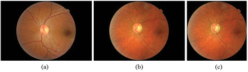
The Optic Disc (OD) has certain features, under healthy and damaged conditions, that can be identified and learned from the fundus images. Figure 1a below shows the normal fundus image while Figure 1b represents a glaucomatous optic disc, and Figure 1c is a glaucomatous disc image with optic disc and optic cup boundaries marked by an expert. Glaucoma diagnosis is typically performed based on the physical evaluation of optic nerve head (ONH) via ophthalmoscopy, the patient’s visual field tests (perimetry), and additional clinical information such as Intraocular Pressure (IOP), etc (Bock et al. 2010). Clinical evaluation of Optic Nerve Head (ONH) is the cornerstone of diagnosing glaucoma (Hussain and Holambe 2015). Further, thinning of Retinal Nerve Fiber Layer (RNFL) is also an indicator of glaucoma which while is clearly visible in Optical Coherence Tomography (OCT) images, is only faintly visible in fundus images. The risk factors associated with glaucoma include age, gender, height, weight, family history with glaucoma (FHG), etc. and systemic diseases like diabetic Mellitus and hypertension (Coleman and Miglior 2008; McMonnies 2017; Alam Miah and Yousuf 2018).

Figure 1. Fundus image (a) healthy eye (b) glaucomatous eye (c) glaucomatous image marked by the expert.

Feature extraction from fundus images

For feature extraction from fundus images, several image processing techniques have been implemented (Khan et al. 2019; Saiteja et al. 2021). Emergence of AI has enabled researchers to use these features in conjunction with machine learning models to help improve glaucoma diagnosis. Machine learning (ML) allows computers to learn from datasets (fundus images in the present case) and make effective predictions (Sarhan et al. 2020). While ML models give the best performances with small datasets, due to manual feature selection from fundus images, the convergence and over-fitting problems in the models are not eliminated. This limits their application and thus use of deep learning (DL) models has become popular due to their robust diagnostic performance in ophthalmic disease classification (Lecun et al. 2015; Bulut et al. 2020). Convolution Neural Networks (CNNs) are DL architectures that can be effectively implemented for medical image segmentation and classification as they can extract features and learn from the pixel intensities of the images (Diaz-Pinto et al. 2019). It may however be noted that while ML models based on radiomic features, generated by the extraction of quantitative features such as, shape features, first-order histogram features, and second-order texture features, etc., provide better explainability (Leandrou et al. 2023; Militello et al. 2023; Prinzi et al. 2023), DL architectures typically have better predictive performance in medical image analysis (Sun et al. 2020; Wei 2021).

The deep CNN model uses more convolution layers to extract features from the raw pixel image data. It can make automated predictions from the input image data using built-in feature extraction property. Since the model should extract all salient features from the fundus images, localisation of the region of interest in the images for better feature selection is the preliminary step before resorting to the deep learning approach. Unlike the approach in current literature (Orlando et al. 2017; Diaz-Pinto et al. 2019; Park et al. 2020) that uses fundus images cropped around the OD or entire fundus image, our work proposes to use images cropped around ONH, which is at the centre of the image as well as the RNFL region that surrounds it even if it appears faint. Further, visualisation by deep network layers has been incorporated to identify the features extracted between the layers to understand the features being looked into by the model.

The main contributions of this work are as follows.

• For better feature selection, we pre-processed the fundus images with a region of interest (ROI) that incorporated the ONH and RNFL region. Experiments have been performed on these images for glaucoma classification.

• We propose a version of deep CNN model to predict the stage of glaucoma (mild, moderate, and severe) based on features typically used by the ophthalmologists and validate the same with those extracted through visualisation by CNN layers.

• The proposed model is compared with ImageNet trained CNN architectures such as VGG16, ResNet50 and MobileNetV2, and it has been observed that our model outperformed these architectures yielding an accuracy of 93.75 %.

The paper is organised as follows: Section 2 summarises the recent literature related to the application of deep learning techniques for glaucoma classification. Section 3 provides details of the deep CNN model deployed by us that has built-in visualisation features. Section 4 describes the ImageNet trained CNN architectures and compares the results obtained with those of our model. Section 5 presents the experimental results obtained with visualisation of features as well as the performance metrics while Section 6 draws conclusions of the work.

Literature survey

Out of all the deep learning approaches for image classification, CNN is the most preferred one since it can learn and extract highly discriminative features from pixel intensities of the image. CNN is used by researchers for medical image analysis and classification and thus it’s no surprise that it is also used for glaucoma detection and classification (Elangovan and Nath 2021; Alayón et al. 2023). A deep learning approach was developed to detect optic disc abnormality and to classify optic disc regions into three classes using four public and four private databases (Alghamdi et al. 2017). The three classes of glaucoma condition used in their approach were normal, suspicious, and abnormal classes. In their work, the optic disc localisation approach used CNN to learn the most informative features from the fundus image. But CNN requires a large amount of labelled data. As a result, training deep CNN from scratch is difficult. However, this was surpassed by using pre-trained CNN with adequate fine-tuning (Tajbakhsh et al. 2017). Two different CNNs were deployed to produce the feature vectors (Orlando et al. 2017). The CNNs used in their work were VGG-S and OverFeat. Pre-processing techniques such as vessel inpainting, contrast limited adaptive histogram equalisation (CLAHE), and cropping around ONH were proposed. However, the main limitation of their work includes a small number of image datasets to test the performance of CNN.

A Glaucoma-Deep system was developed that implemented an unsupervised CNN architecture which automatically extracts features through a multilayer from raw pixel intensities of colour fundus images (Abbas 2017). Here, a deep-belief network (DBN) model was used to select the most discriminative features from the CNN model. In their model, retinal images from three public and one private database were used to evaluate the performance using statistical measures like sensitivity (SE), accuracy (ACC), specificity (SP), and precision (PRC).

For automatic glaucoma assessment using retinal fundus images, five different ImageNet trained models were employed (Diaz-Pinto et al. 2019). Extensive validation of CNNs was done in their work. Images were taken from ACRIMA, the largest public database for glaucoma diagnosis, and out of the ImageNet trained models (InceptionV3, VGG16, VGG19, Xception, and ResNet50), the Xception architecture resulted in the best performance. CDR detection and ONH localisation was developed using state-of-the-art DL architectures such as YOLO V3, ResNet, and DenseNet to compare various aspects of performance other than the classification accuracy (Park et al. 2020). The performance measures discussed in their work included processing time, image resolution, and diagnostic performance. An ensemble of deep convolutional networks using stacking ensemble learning technique was developed for glaucoma detection (Elangovan and Nath 2022). Their approach was implemented with thirteen pre-trained models such as Alexnet, VGG-16, VGG-19, Googlenet, Resnet-18, Resnet-50, Resnet-101, Squeezenet, Mobilenet-v2, Efficientnet-b0, Inception-v3, Xception and Densenet-201 on modified publicly available databases such as DRISHTI-GS1-R, ORIGA-R, RIM-ONE2-R, LAG-R, and ACRIMA-R. A DL approach was developed for pathological area localisation and diagnosis of glaucoma (Li et al. 2020). An attention-based CNN (AG-CNN) using large-scale attention-based glaucoma (LAG) database for glaucoma classification was established, and further, performance metrics were also evaluated. Optic disc and optic cup segmentation was performed using deep learning convolutional network in the work by the authors (Juneja et al. 2020). The authors used small dataset and a deep learning architecture was developed with CNN for automating glaucoma detection. Statistical parameters such as cup entropy and kurtosis from colour fundus images were measured in the work by (Elangovan et al. 2020) using FCM algorithm based on morphological reconstruction and membership filtering (FRFCM). They implemented the algorithm on publicly available RIM-ONE and DRIONS-DB databases which produced better results than CDR-based glaucoma classification. Segmentation and classification of glaucoma was implemented using U-Net architecture with deep CNN model in the work by (Sudhan et al. 2022). The model used ORIGA dataset and deep CNN (DCNN) approach was used for classification of glaucoma. In all the research work reported above, deep learning approach was used on public or private datasets to extract features in an attempt for efficient classification. It appears however that feature visualisation from fundus images for glaucoma detection has not been attempted.

A deep learning model was investigated to identify the best X-ray features for COVID-19 detection in the work by (Apostolopoulos et al. 2022). The grad-CAM algorithm was used to visualise the areas of the images in their work. To efficiently interpret and diagnose glaucoma, an explainable machine learning model was developed in the work by (Oh et al. 2021). They designed a system called Magellan that produced explainable results in the prediction of glaucoma. Glaucoma prediction analysis was evaluated using an explainable artificial intelligence model in the work by (Kamal et al. 2022). The author proposed explainable artificial intelligence and interpretable machine learning model to generate trustworthy predictions for glaucoma. However, in the above works, feature visualisation appears to have played a lesser role in glaucoma detection and classification. A major focus of this work is the visualisation of features between layers of our deep CNN model and utilisation of the same for glaucoma classification.

Methodology

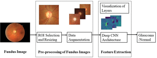
Our approach is to take advantage of the visualisation ability of deep CNN layers while assessing the features of fundus images. Accordingly, the whole dataset is pre-processed to the required size and resolution. Also, the dataset is augmented to increase the number of images. These images are fed to the deep CNN architecture with four convolutional layers and two dense layers for the classification of glaucoma and normal images. Visualisation of the features is carried out in between the layers which gives us clarity on the features extracted from within the layers. The proposed methodology is depicted in Figure 2 while details of pre-processing of the fundus dataset and deep CNN architecture are provided in the subsections below.

Figure 2. Proposed deep CNN model with visualization of features.

Dataset

The fundus dataset considered in this work consists of 295 normal images and 120 glaucomatous images which are part of a project carried out by L.V. Prasad Eye Institute, based in Hyderabad, India. Normal fundus images are divided, based on the optic disc size, into large, medium and small with a count of 96, 100, and 99, respectively. Similarly, optic discs were divided into small (<1.6 mm²), average (1.6–2.6 mm²) and large (>2.6 mm²) (Rao et al. 2009). Glaucomatous images have been divided into mild, moderate and severe based on the severity of damage (based on visual field severity grading done by trained glaucoma specialist). Severity of glaucoma is assessed based on visual fields mean deviation (MD), viz., mild: MD better than −6 dB, moderate: MD between −6 dB and −12 dB and severe: MD worse than −12 dB, known as Hoddap-Parrish-Anderson criteria (E et al. 1993). They are of a total count of 10, 23, and 29, respectively. The original image resolution is 3216 × 2136 which is very large for any deep learning model to handle. Hence, we have pre-processed the entire image dataset to a manageable size.

Preprocessing of fundus dataset

Selection of region of interest

The region of interest (ROI) from fundus images is chosen in such a way that important features related to glaucoma are retained. Pre-processing of images was carried out using Python and the OpenCV library. The first step in preprocessing is to remove the redundant portions of the fundus image followed by cropping around OD, cropping around ONH while retaining the RNFL region, segmented optic disc, as well as using the full fundus image in its entirety. These methods are illustrated in Figure 3 for a glaucomatous fundus image.

Figure 3. Pre-processing of fundus image with glaucoma (a) entire image (b) fundus image cropped around OD (c) fundus glaucoma image cropped around ONH including RNFL region (d) segmented optic disc region.

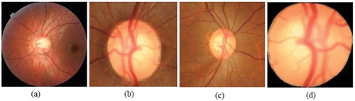
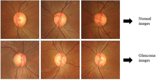
The features relevant for glaucoma diagnosis are those that surround the optic disc and the peripapillary (around the optic disc) RNFL. Thus, out of the four types of pre-processed images, cropping around ONH that includes RNFL region, has been chosen for feature extraction and classification as explained in (Jisy et al. 2024). Subsequently, the fundus images have been resized to 256 × 256 and labelled appropriately before being given as input to our deep CNN model. A sample of the cropped and resized images is shown in Figure 4 below. This downscaled resolution helps to reduce the time complexity of computation.

Figure 4. Examples of the ROI in the fundus images cropped around the ONH including RNFL region for both normal and glaucomatous images.

Data augmentation

Since the dataset is of a smaller size, we performed data augmentation to increase the number of images for training and testing the model. Data augmentation can be performed by several transformations on the image or by synthetically generating images using techniques such as generative adversarial networks (GAN) (Nandhini Abirami et al. 2021). We have augmented the dataset by image transformations like flipping horizontally, flipping vertically, and rotating the image by 90°, 180°, and 270°. These techniques are applied to all the classes of glaucoma image datasets. In our architecture dropout layers and normalisation terms are also added. The number of images obtained after augmentation is presented in Table 1 below.

Table 1. Fundus dataset before and after augmentation.

Fundus glaucoma class	Total images	Images after augmentation
Mild	10	50
Moderate	23	118
Severe	29	137

The deep CNN architecture

The proposed architecture uses four convolutional layers (four convolution layers + four max pooling layers) and two fully connected layers. This is depicted in Figure 5. According to the input image dataset, the number of layers and filter sizes are selected appropriately such that the number of parameters involved in the design is also optimised. The input image size is 256 × 256 × 3 representing the image dimensions, height x width x channel.

Figure 5. The proposed deep CNN architecture.

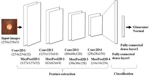
We chose the ReLU activation function for all convolution layers as it helps in vanishing gradient problems in which useful gradient information is unable to propagate from output to input. Dropout layers are also implemented in between the layers to reduce the overfitting problem. The fully connected output layer uses the softmax activation function. More number of parameters are involved in the implementation of this layer as each neuron in this layer is connected to all the neurons in the previous layers. While training the network, the loss function used is categorical cross entropy with RMSprop optimiser. The learning rate is 0.0001 which helps to achieve the minimum cost function. The network was trained for 100 epochs with a batch size of 16. The steps per epoch while training the model are chosen according to the batch size. All these hyperparameters are effectively selected, and the weights or system parameters are updated and saved appropriately. The details of kernel size and filter size are mentioned in Table 2. Also, visualisation of features within the layers was resorted to and observed accordingly.

Table 2. Details of the proposed deep CNN architecture.

Layers	Kernels	Filter size	Output shape
Conv2D 1	32	3 x 3	254 x 254 x 32
MaxPool2D 1	32	2 x 2	127 x 127 x 32
Conv2D 2	64	3 x 3	125 x 125 x 64
MaxPool2D 2	64	2 x 2	62 x 62 x 64
Conv2D 3	128	3 x 3	60 x 60 x 128
MaxPool2D 3	128	2 x 2	30 x 30 x 128
Conv2D 4	256	3 x 3	28 x 28 x 256
MaxPool2D 4	256	2 x 2	14 x 14 x 256
Flatten	–	–	50176
Fully connected Dense1	256	–	256
Fully connected Dense2	2	–	2

Performance metrics

The results are evaluated by computing performance measures such as accuracy, specificity, sensitivity, precision, F1 score and Matthews Correlation Coefficient (MCC). The true positive (TP), false positive (FP), true negative (TN), and false negative (FN) values are identified to define the performance metrics. TP is glaucoma image being identified as glaucoma, TN is the healthy image being identified as healthy, FP is a false glaucoma prediction which means normal is identified as glaucoma and FN is a false normal prediction in which glaucoma is identified as normal. The equations for evaluating the accuracy, specificity, sensitivity, precision, F1 score and MCC are given below (Bogacsovics et al. 2022; Anbalagan et al. 2023)

(1) $\mathit{Accuracy}=\mathit{\hspace{0.17em}}\frac{\mathit{TP}+\mathit{TN}}{\mathit{TP}+\mathit{FN}+\mathit{TN}+\mathit{FP}}$(1)

(2) $\mathit{Sensitivity}=\mathit{\hspace{0.17em}}\frac{\mathit{TP}}{\mathit{TP}+\mathit{FN}}$(2)

(3) $\mathit{Specifity}=\mathit{\hspace{0.17em}}\frac{\mathit{TN}}{\mathit{TN}+\mathit{FP}}$(3)

(4) $\mathit{Precision}=\mathit{\hspace{0.17em}}\frac{\mathit{TP}}{\mathit{TP}+\mathit{FP}}$(4)

(5) $\mathit{F}1\mathit{\hspace{0.17em}}\mathit{score}=\mathit{\hspace{0.17em}}\frac{2\ast p\mathrm{recision}\ast s\mathrm{ensitivity}}{\mathit{precision}+\mathit{sensitivity}}=\frac{2\ast TP}{2\ast TP+FP+FN}$(5)

(6) $\mathit{MCC}=\frac{\mathit{TP}.\mathit{TN}-\mathit{FP}.\mathit{FN}}{\sqrt{\left(\mathit{TP}+\mathit{FP}\right).\left(\mathit{TP}+\mathit{FN}\right).\left(\mathit{TN}+\mathit{FP}\right).\left(\mathit{TN}+\mathit{FN}\right)}}$(6)

ImageNet trained CNN architectures

CNN architecture has evolved from a few layers to multiple layers in the past few years to extract high level features of the application on hand. ImageNet is a large database of images that comprises of millions of annotated images segregated into different classes. Making use of this database in the annual ImageNet Large Scale Visual Recognition Challenge (ILSVRC), the performance of ImageNet trained CNN architectures has been evaluated (Russakovsky et al. 2015). Such ImageNet trained models have been used in glaucoma disease classification (Diaz-Pinto et al. 2019; Park et al. 2020; Bogacsovics et al. 2022). But the results and model performance vary according to the specific features selected and the datasets used for training. In this work, we compared the results obtained for different glaucoma classes with three ImageNet trained architectures, viz., VGG16, ResNet50 and MobileNetV2. The models were selected for comparison by looking into the depth of the layers and their performances in medical image analysis. VGG16 architecture is 16 layers deep (13 convolutional layers + 5 maxpooling layers + 3 dense layers) that contributes to the learnable parameters in the network (Simonyan and Zisserman 2015). The convolution layer is a 3 × 3 filter with stride 1 that uses same padding while maxpool layer is 2 × 2 filter with stride 2. ResNet50 architecture is 50 layers deep that comprises of convolutional blocks and identity blocks. This architecture reduces the vanishing gradient problem encountered with VGG16 networks and also the number of trainable parameters is less than VGG16 model (Khan et al. 2020). MobileNetV2 is a CNN architecture which is 53 layers deep. The architecture includes depth wise separable convolutions with linear bottlenecks. Information within convolution layers is retained in the inverted residual blocks (Sandler et al. 2018). The model performed well for image classification (Dong et al. 2020). All the models help to extract features and classify the image dataset using transfer learning (TL) approach.

Transfer learning

Transfer learning (TL) is a technique of transferring the knowledge learned from training a model in one domain to a different domain. The local features such as edges and corners of the images can be captured by this method using pre-trained weights obtained from the architectures (Yosinski et al. 2014). This helps to reduce the training time and data required. The VGG16, ResNet50 and MobileNetV2 architectures with pre-trained weights are used to extract features. Fine tuning these models as a classifier generating softmax probabilities is carried out to reduce the number of trainable parameters. The process of training and updating the pre-trained weights of CNN using backpropagation is called fine-tuning. When the dataset is small, this method can be adopted for medical image classification (Tajbakhsh et al. 2017). Initial layers are frozen for all the models used and the final fully connected layers are replaced with new fully connected dense layer with 2-class classification task. The newly added layers are trained as a part of fine-tuning. The list of hyperparameters used for the VGG16, ResNet50 and MobileNetV2 architectures is summarised in Table 3 below.

Table 3. The list of hyperparameters for the ImageNet trained architectures.

Type of glaucoma	Network	Optimizer	Batch size	Learning rate	Epochs
Mild	VGG16	Adam	16	0.001	100
	ResNet50	Adam	16	0.001	100
	MobileNetV2	Adam	32	0.0001	50
	Proposed Deep CNN	RMSprop	16	0.0001	100
Moderate	VGG16	Adam	32	0.0001	100
	ResNet50	Adam	32	0.0001	100
	MobileNetV2	Adam	32	0.0001	100
	Proposed Deep CNN	RMSprop	16	0.0001	100
Severe	VGG16	Adam	32	0.0001	100
	ResNet50	Adam	32	0.0001	100
	MobileNetV2	Adam	32	0.0001	100
	Proposed Deep CNN	RMSprop	16	0.0001	100

Experimental results and discussion

The deep CNN architecture proposed is trained and tested using the dataset mentioned in Table 1. We have a fundus dataset of 295 normal images out of which we have taken images in such a way that during training and validation the class imbalance problem is eliminated. This helps to reduce overfitting and results in better accuracy. Out of total images, 70% are used for training and 30% are used for testing the model. From the training set 10% of images are used for validation. The number of images of normal and three classes of glaucoma used for training and testing are shown in Table 4.

Table 4. Total images used for training and testing the architecture.

Glaucoma classes	Glaucoma images	Normal images	Total
Mild	50	60	110
Moderate	118	120	238
Severe	137	140	277

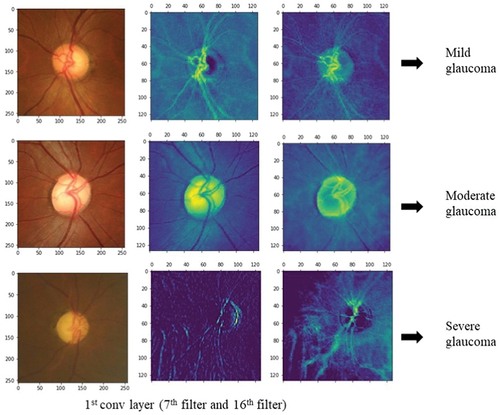
The deep CNN architecture model is implemented with Python programming language using the Keras library in Google Colab. The outputs from the layers of deep CNN are visually represented to analyse the feature extracted from within these layers. Since the most important features lie around the optic disc, the fundus image features are visually represented to find out if the model is extracting the features relevant to glaucoma or not. This helps to understand which features of the input image are detected and preserved in the feature maps obtained. While visualising from the first layer of convolution to the output layer, the feature maps in the starting layers detect finer details whereas feature maps closer to the output layers detect global features. The first layer of activation has 32 filters and hence 32 channel feature maps can be plotted. This number increases as the number of filters and layers increases. Thus, we have plotted some feature maps in the first layer of convolution as depicted in Figure 6. The feature maps convey that the convolution layers followed by max-pooling layers are detecting the optic disc boundaries, brighter optic cup region, blood vessels (though not relevant to glaucoma), and retinal nerve fibre layers. The model can be trained in such a way that all the relevant features are extracted efficiently for a better discrimination of glaucoma from the normal class.

Figure 6. Visualization of the feature maps of first layer of activation. The first row is a feature map of mild glaucoma, the second row is moderate glaucoma, and the third row is severe glaucoma. The feature maps are plotted for the 7^th and 16^th channels which are taken randomly out of the 32 channels in the first activation layer.

The training and validation accuracy curves and loss curves of mild, moderate, and severe glaucoma classes are plotted as shown in Figures 7, 8, 9 respectively as well as accuracy for all classes is calculated. For the mild glaucoma class, the training accuracy obtained is 85.7% while validation accuracy is 87.8%. Similarly, the training and validation accuracy for moderate and severe glaucoma classes are 92.8% and 94.3%, and 93.8% and 89.1%, respectively. These values are marked in Table 5.

Figure 7. Accuracy curve and loss curve of mild glaucoma class.

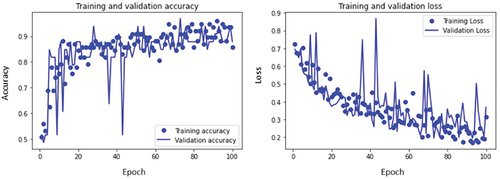
Figure 8. Accuracy curve and loss curve of moderate glaucoma class.

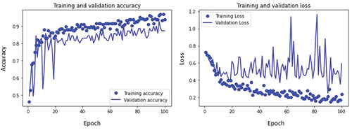
Figure 9. Accuracy curve and loss curve of severe glaucoma class.

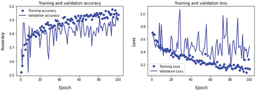
Table 5. Training and validation accuracy of glaucoma dataset.

Glaucoma class	Training accuracy	Validation accuracy	Training loss	Validation loss
Mild	85.71	87.88	0.31	0.36
Moderate	92.81	94.37	0.17	0.23
Severe	93.8	89.1	0.12	0.48

Confusion matrices for all classes are computed to evaluate the performance of the model. From these matrices depicted in Figure 10, accuracy, specificity, sensitivity, precision, F1 score and MCC have been calculated as shown in Table 6. The values obtained help us to understand if the model is discriminating between the glaucoma and normal classes correctly. For a model to perform well, the range of values for F1 score (which is the weighted average of sensitivity or recall and precision) should be between 0 and 1, 0 being the worst performance and 1 giving the best. It can be seen from Table 6 that mild, moderate and severe glaucoma classes have values of 0.94, 1, and 0.95 respectively indicating that the model is able to discriminate between the classes well.

Figure 10. Confusion matrices for (a) mild glaucoma (b) moderate glaucoma (c) severe glaucoma.

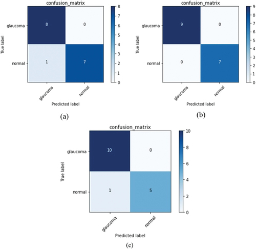
Table 6. Results of performance metrics evaluated for the deep CNN architecture.

Glaucoma class	Accuracy (%)	Sensitivity (%)	Specificity (%)	Precision (%)	F1-score	MCC
Mild	93.75	100	87.5	88.8	0.94	+0.88
Moderate	100	100	100	100	1	+1
Severe	93.75	100	83.3	90.9	0.95	+0.87

Further, related to another important metric, the Mathew’s Correlation Coefficient (MCC), if the binary classifier predicts a majority of positive and negative instances accurately, it generates a high score. The range of MCC is typically between −1 and + 1, with former indicating the worst value and the latter the best. Our model generated MCC of + 0.88, +1 and + 0.87 for mild, moderate and severe glaucoma, respectively, which is consistent with other metrics. Overall, the accuracy, F1-score and MCC show reliable scores for predictions that accurately classify the positive and negative classes.

Comparison with ImageNet trained CNN architectures

The mild, moderate, and severe classes of glaucoma are classified using state-of-the-art networks like VGG16, ResNet50, and MobileNetV2 and compared with the proposed deep CNN model for all the classes. The input fundus images are resized to 224 × 224 * 3 before being input to all these architectures. The visual representation of the outcome of the layers of deep CNN model proposed gave us insight into the local features such as edges, corners of the optic disc (related to neuro-retinal rim), and RNFL region within the fundus images. The performance metrics are reported in Table 6. The ImageNet trained CNN architectures used also were pretrained and finetuned to extract features and classify the fundus image datasets. The test accuracy obtained with these architectures for each class of glaucoma against the normal class and their comparison with the proposed CNN model are depicted in Table 7. The results indicate that, in the mild class of glaucoma images the features are not so prominent leading to the model giving an accuracy of 93.75% which is better when compared to models such as VGG16, ResNet50, and MobileNetV2. Further, while the moderate class gives an accuracy of 100%, the severe class of glaucoma images gave an accuracy of only 93.75% which is same as that of the mild class. This can be understood from the images shown in Figure 6 where a prominent feature relevant to glaucoma, the RNFL thickness (thinning of which is strongly correlated with the presence of glaucoma), can be prominently seen in the moderate class but which appears obliterated in the severe class of glaucoma images.

Table 7. Comparison of result of test accuracy for proposed deep CNN model and ImageNet trained architectures.

Glaucoma	VGG16	ResNet50	MobileNetV2	Proposed deep CNN model
Class	Test Accuracy (%)	Test Accuracy (%)	Test Accuracy (%)	Test Accuracy (%)
Mild	84.09	81.82	75	93.75
Moderate	89.13	97.83	89.03	100
Severe	97.03	93.07	94.06	93.75

Comparison with existing work

Since a considerable body of the literature exists on fundus image classification for glaucoma, the work reported here has been compared with the existing literature. The following Table 8 provides this comparison.

Table 8. Comparison of performance metrics evaluated for the existing models vs proposed model.

Model	ACC (%)	SE (%)	SP (%)	PRC (%)	F1-score	MCC
(Diaz-Pinto et al. 2019)	80.00	83.33	77.78	-	-	-
(Elangovan and Nath 2021)	96.64	96.07	97.39	97.74	-	-
(Li et al. 2020)	85.20	84.80	85.50	-	-	-
(Alghamdi et al. 2017)	86.52	96.42	86.00	-	-	-
Proposed	93.75	100	87.5	88.8	0.94	+0.88

It can be seen from the table that certain metrics computed using our model compare favourably with those of (Elangovan and Nath 2021) who appear to have reported the best results. However, they have not reported certain metrics such as F1-score and MCC as done by us. It must also be emphasised that while these authors have used the publicly available datasets, our dataset is a specialised one available with an eye institute. Thus, a direct comparison of results may not be very appropriate.

Conclusion

Detection of glaucoma is important due to the progressive nature of this ocular disease. If not detected and treated at the right time, glaucoma can lead to a loss of vision and later to permanent blindness. In this paper, we implemented a deep CNN architecture with visualisation of features to distinguish between glaucomatous and healthy fundus images. We attempted visualisation between the layers of CNN to identify the features extracted and they turned out to be similar to those considered by the clinicians while diagnosing for glaucoma. However in practice, the clinicians also perform other tests such as HVF (Humphrey Visual Field) test to distinguish between mild, moderate and severe glaucoma which are not built into the current model. Thus, there is a limit on the accuracy of prediction which turned out to be still high at 93.75% (on the lower side) in this work.

Disclosure statement

No potential conflict of interest was reported by the author(s).

Additional information

Notes on contributors

Jisy N K

Jisy N K is a Ph.D. student in the Department of Electrical and Electronics Engineering at Birla Institute of Technology and Science (BITS) Pilani, Hyderabad Campus, India. She received her B.Tech degree in Electronics and Communication Engineering from AWH Engineering College, Kerala, India in 2009 and her Masters degree in VLSI design from Anna University Regional Centre, Coimbatore, India in 2013. She was honored with the College Topper Award in 2010 and was a Rank holder in her ME VLSI Design program in 2013. Her current research interests include biomedical image processing, application of machine learning, and deep learning for fundus image processing.

Md. Hasnat Ali

Dr. Md Hasnat Ali completed his Ph.D. from Birla Institute of Technology and Science (BITS) Pilani, Hyderabad Campus from the Department of Electrical and Electronics Engineering. He is currently the senior bio-statistician at L V Prasad Eye Institute. He has been an integral part of the institute’s faculty since 2010, bringing his expertise and knowledge to advance research and statistical analysis in the field of ophthalmology. He has demonstrated exceptional proficiency in designing robust statistical models, analyzing complex data sets, and interpreting results precisely. He received his MBA in Public Health Informatics from Jamia Hamdard, university, New Delhi. His research interests include circular and functional data analysis, computational statistics and machine learning, predictive modeling, and Big data analysis. He has published in over 150 international publications as an author or co-author.

Sirisha Senthil

Dr. Sirisha Senthil is a highly accomplished Ophthalmologist with over 22 years of experience in the field of Glaucoma. She holds an MS in Ophthalmology from Aravind Eye Hospital, Madurai, and an FRCS in Ophthalmology from Edinburgh. She is currently the Head of Glaucoma service at L V Prasad Eye Institute, where she has been a faculty member since 2007. Dr. Senthil specializes in managing refractory adult and pediatric glaucomas, with a particular interest in glaucoma drainage implants and secondary glaucomas and genetics of inherited childhood glaucoma. She has published over 186 scientific papers in peer-reviewed journals, authored several book chapters and received multiple awards in national and international fora for her work, including Dr. Vengal Rao Medal in 2012, IJO Silver award in 2016, and the American Academy of Ophthalmology Achievement award in 2018.

M.B. Srinivas

M.B. Srinivas received his Ph.D. in Electrical Engineering from the Indian Institute of Science, Bangalore, India. He is currently a Professor in the Department of Electrical and Electronics Engineering at Birla Institute of Technology and Science (BITS) Pilani. His research interests include Computer Arithmetic and Architectures, Medical Device Design and Deep Learning Models for Medical Image Processing. He was a recipient of Microsoft Research ’Digital Inclusion’ award in 2006 and Stanford Medicine ’MedTech Innovation’ award in 2016.

References

- Abbas Q. 2017. Glaucoma-Deep: detection of Glaucoma eye disease on retinal fundus images using Deep learning. Int J Advan Comput Sci Appl. 8(6):41–12. doi: 10.14569/ijacsa.2017.080606.
- Alam Miah MB, Yousuf MA. 2018. Analysis the significant risk factors on type 2 diabetes perspective of Bangladesh. Diabetes Metab Syndr. 12(6):897–902. doi: 10.1016/j.dsx.2018.05.012.
- Alayón S, Hernández J, Fumero FJ, Sigut JF, Díaz-Alemán T. 2023. Comparison of the performance of convolutional neural networks and vision transformer-based systems for automated glaucoma detection with eye fundus images. Appl Sci. 13(23):12722. doi: 10.3390/app132312722.
- Alghamdi HS, Tang HL, Waheeb SA, Peto T. 2017. Automatic optic disc abnormality detection in fundus images: a deep learning approach. 17–24. 10.17077/omia.1042.
- Anbalagan T, Nath MK, Vijayalakshmi D, Anbalagan A. 2023. Analysis of various techniques for ECG signal in healthcare, past, present, and future. Biomed Eng Adv. 6(April):100089. doi: 10.1016/j.bea.2023.100089.
- Apostolopoulos ID, Apostolopoulos DJ, Papathanasiou ND. 2022. Deep learning methods to reveal important X-ray features in COVID-19 detection: investigation of explainability and feature reproducibility. Reports. 5(2):20. doi: 10.3390/reports5020020.
- Bernardes R, Serranho P, Lobo C. 2011. Digital ocular fundus imaging: a review. Ophthalmologica. 226(4):161–181. doi: 10.1159/000329597.
- Bock R, Meier J, Nyúl LG, Hornegger J, Michelson G. 2010. Glaucoma risk index: Automated glaucoma detection from color fundus images. Med Image Anal. 14(3):471–481. doi: 10.1016/j.media.2009.12.006.
- Bogacsovics G, Toth J, Hajdu A, Harangi B. 2022. Enhancing CNNs through the use of hand-crafted features in automated fundus image classification. Biomed Signal Process Control. 76(October 2021):103685. doi: 10.1016/j.bspc.2022.103685.
- Bulut B, Kalin V, Gunes BB, Khazhin R. 2020. Deep learning approach for detection of retinal abnormalities based on color fundus images. In: Proceedings - 2020 Innovations in Intelligent Systems and Applications Conference, ASYU 2020. doi: 10.1109/ASYU50717.2020.9259870.
- Coleman AL, Miglior S. 2008. Risk factors for glaucoma onset and progression. Surv Ophthalmol. 53(6 SUPPL):3–10. doi: 10.1016/j.survophthal.2008.08.006.
- Diaz-Pinto A, Morales S, Naranjo V, Köhler T, Mossi JM, Navea A. 2019. Cnns for automatic glaucoma assessment using fundus images: an extensive validation. Biomed Eng Online. 18(1):1–19. doi: 10.1186/s12938-019-0649-y.
- Dimitriou CD, Broadway DC. 2013. Pathophysiology of glaucoma. Glaucoma: Basic Clin Perspect. 33–57. doi: 10.2217/EBO.12.421.
- Dong K, Zhou C, Ruan Y, Li Y. 2020. MobileNetV2 model for image classification. In: Proceedings - 2020 2nd International Conference on Information Technology and Computer Application, ITCA 2020 p. 476–480. 10.1109/ITCA52113.2020.00106.
- E H, II PR, DR A. 1993. Clinical decisions in glaucoma. St Louis: The CV Mosby Co.
- Elangovan P, Nath MK. 2021. Glaucoma assessment from color fundus images using convolutional neural network. Int J Imaging Syst Technol. 31(2):955–971. doi: 10.1002/ima.22494.
- Elangovan P, Nath MK. 2022. En-ConvNet: a novel approach for glaucoma detection from color fundus images using ensemble of deep convolutional neural networks. Int J Imaging Syst Technol. 32(6):2034–2048. doi: 10.1002/ima.22761.
- Elangovan P, Nath MK, Mishra M. 2020. Statistical parameters for glaucoma detection from color fundus images. Procedia Comput Sci. 171(2019):2675–2683. doi: 10.1016/j.procs.2020.04.290.
- Hussain SA, Holambe AN. 2015. Automated detection and classification of glaucoma from eye fundus images: a survey. Int J Comput Sci Inf Technol. 6(2):1217–1224.
- Jisy NK, Md HA, Senthil S, Srinivas MB. 2024. Localization of region of interest from retinal fundus image for early detection of glaucoma. Located: Proc Ninth Int Congr Inf Commun Technol: ICICT 2024. 6. London, Singapore: Springer.
- Johora FT, Mahbub -Or-Rashid M, Yousuf MA, Saha TR, Ahmed B. 2020. Diabetic retinopathy detection using PCA-SIFT and weighted decision tree. January. 2020:25–37. doi: 10.1007/978-981-13-7564-4_3.
- Juneja M, Singh S, Agarwal N, Bali S, Gupta S, Thakur N, Jindal P. 2020. Automated detection of Glaucoma using deep learning convolution network (G-net). Multimedia Tools Appl. 79(21–22):15531–15553. doi: 10.1007/s11042-019-7460-4.
- Kamal MS, Dey N, Chowdhury L, Hasan SI, Santosh KC. 2022. Explainable AI for glaucoma prediction analysis to understand risk factors in treatment planning. IEEE Trans Instrum Meas. 71:1–9. doi: 10.1109/TIM.2022.3171613.
- Khan KB, Khaliq AA, Jalil A, Iftikhar MA, Ullah N, Aziz MW, Ullah K, Shahid M. 2019. A review of retinal blood vessels extraction techniques: challenges, taxonomy, and future trends. Pattern Anal Applic. 22(Issue 3):767–802. Springer London. doi: 10.1007/s10044-018-0754-8.
- Khan A, Sohail A, Zahoora U, Qureshi AS. 2020. A survey of the recent architectures of deep convolutional neural networks. Artif Intell Rev. 53(Issue 8):5455–5516. Springer Netherlands. doi: 10.1007/s10462-020-09825-6.
- Leandrou S, Lamnisos D, Bougias H, Stogiannos N, Georgiadou E, Achilleos KG, Pattichis CS. 2023. A cross-sectional study of explainable machine learning in Alzheimer’s disease: diagnostic classification using MR radiomic features. Front Aging Neurosci. 15(June):1–11. doi: 10.3389/fnagi.2023.1149871.
- Lecun Y, Bengio Y, Hinton G. 2015. Deep learning. Nature. 521(7553):436–444. doi: 10.1038/nature14539.
- Li L, Xu M, Liu H, Li Y, Wang X, Jiang L, Wang Z, Fan X, Wang N. 2020. A large-scale database and a CNN model for attention-based glaucoma detection. IEEE Trans Med Imaging. 39(2):413–424. doi: 10.1109/TMI.2019.2927226.
- McMonnies CW. 2017. Historial de glaucoma y factores de riesgo. [Glaucoma history and risk factors]. J Optom. 10(2):71–78. Spanish. 10.1016/j.optom.2016.02.003.
- Militello C, Prinzi F, Sollami G, Rundo L, La Grutta L, Vitabile S. 2023. CT radiomic features and clinical biomarkers for predicting coronary artery disease. Cognit Comput. 15(1):238–253. doi: 10.1007/s12559-023-10118-7.
- Nandhini Abirami R, Durai Raj Vincent PM, Srinivasan K, Tariq U, Chang CY, Sarfraz DS. 2021. Deep CNN and deep GAN in computational visual perception-driven image analysis. Complexity. 2021:1–30. doi: 10.1155/2021/5541134.
- Oh S, Park Y, Cho KJ, Kim SJ. 2021. Explainable machine learning model for glaucoma diagnosis and its interpretation. Diagnostics. 11(3):1–14. doi: 10.3390/diagnostics11030510.
- Orlando JI, Prokofyeva E, Del Fresno M, Blaschko MB. 2017. Convolutional neural network transfer for automated glaucoma identification. 12th Int Symp Med Inf Proc Anal. 10160:101600U. doi: 10.1117/12.2255740.
- Park K, Kim J, Lee J. 2020. Automatic optic nerve head localization and cup-to-disc ratio detection using state-of-the-art deep-learning architectures. Sci Rep. 10(1):3–12. doi: 10.1038/s41598-020-62022-x.
- Prinzi F, Militello C, Scichilone N, Gaglio S, Vitabile S. 2023. Explainable machine-learning models for COVID-19 prognosis prediction using clinical, laboratory and radiomic features. IEEE Access. 11(October):121492–121510. doi: 10.1109/ACCESS.2023.3327808.
- Rao HBL, Sekhar GC, Babu GJ, Parikh RS. 2009. Clinical measurement and categorization of optic disc in glaucoma patients. Indian J Ophthalmol. 57(5):361–364. doi: 10.4103/0301-4738.55075.
- Russakovsky O, Deng J, Su H, Krause J, Satheesh S, Ma S, Huang Z, Karpathy A, Khosla A, Bernstein M, et al. 2015. ImageNet large scale visual recognition challenge. Int J Comput Vision. 115(3):211–252. doi: 10.1007/s11263-015-0816-y.
- Saiteja KV, Kumar PM, Chandra PS, Jisy NK, Ali MH, Srinivas MB. 2021. Glaucoma - automating the cup-to-disc ratio estimation in fundus images by combining random walk algorithm with otsu thresholding. Int IEEE/EMBS Conf Neural Eng, NER. 2021(May):154–157. doi: 10.1109/NER49283.2021.9441435.
- Sandler M, Howard A, Zhu M, Zhmoginov A, Chen LC. 2018. MobileNetV2: inverted residuals and linear bottlenecks. In: Proceedings of the IEEE Computer Society Conference on Computer Vision and Pattern Recognition p. 4510–4520. 10.1109/CVPR.2018.00474.
- Sarhan MH, Nasseri MA, Zapp D, Maier M, Lohmann CP, Navab N, Eslami A. 2020. Machine learning techniques for ophthalmic data processing: a review. IEEE J Biomed Health Inf. 24(12):3338–3350. doi: 10.1109/JBHI.2020.3012134.
- Simonyan K, Zisserman A. 2015. Very deep convolutional networks for large-scale image recognition. In: 3rd International Conference on Learning Representations, ICLR 2015 - Conference Track Proceedings, San Diego, CA, USA, p. 1–14.
- Sudhan MB, Sinthuja M, Pravinth Raja S, Amutharaj J, Charlyn Pushpa Latha G, Sheeba Rachel S, Anitha T, Rajendran T, Waji YA, Abdulhay E. 2022. Segmentation and classification of glaucoma using U-Net with deep learning model. J Healthc Eng. 2022:1–10. doi: 10.1155/2022/1601354.
- Sun Q, Lin X, Zhao Y, Li L, Yan K, Liang D, Sun D, Li ZC. 2020. Deep learning vs. Radiomics for predicting axillary lymph node metastasis of breast cancer using ultrasound images: don’t forget the peritumoral region. Front Oncol. 10(January):1–12. doi: 10.3389/fonc.2020.00053.
- Tajbakhsh N, Shin JY, Gurudu SR, Hurst RT, Kendall CB, Gotway MB, Liang J. 2017. Convolutional neural networks for medical image analysis: full training or fine tuning? ArXiv. 35(5):1299–1312. doi: 10.1109/TMI.2016.2535302.
- Wei P. 2021. Radiomics, deep learning and early diagnosis in oncology. Emerging Top Life Sci. 5(6):829–835. doi: 10.1042/ETLS20210218.
- Yosinski J, Clune J, Bengio Y, Lipson H. 2014. How transferable are features in deep neural networks? Adv Neural Inf Process Syst. 4(January):3320–3328.