Inferring 3D finger bone shapes from 2D images – a detailed analysis of shape accuracy

ABSTRACT

3D visualisation and modelling of anatomical structures of the human body play a significant role in diagnosis, computer-aided surgery, surgical planning, and patient follow-up. However, 2D X-ray images are often used in clinical routine. We propose and validate a method for reconstructing 3D shapes from 2D X-ray scans. This method comprises automatic segmentation and labelling, automated construction of 3D statistical shape models (SSM), and automatic fitting of the SSM to standard 2D X-ray images. This workflow is applied to finger bone shape reconstruction and validated for each finger bone using a set of five synthetic reference configurations and 34 CT/X-ray data pairs. We reached submillimetre accuracy for 91.59% of the synthetic data, while 79.65% of the clinical cases show surface errors below 2 mm. Thus, applying the proposed method can add valuable 3D information where 3D imaging is not indicated. Moreover, 3D imaging can be avoided if the 2D-3D reconstruction accuracy is sufficient.

KEYWORDS:

• Statistical shape model
• 2D-3D reconstruction
• image-based geometric modelling
• shape reconstruction

1. Introduction

Three-dimensional (3D) imaging has reached high importance in today’s clinical routine. There are plenty applications of 3D imaging such as the diagnosis of diseases, computer-aided surgery, surgical planning, patient follow-up, or the design of patient-specific implants. Unfortunately, current waiting times for 3D medical imaging such as magnetic resonance imaging (MRI) or computed tomography (CT) reach up to 90 days (OECD 2020). This leads to delays in the diagnosis and treatment of patients with adverse effects for the patient. Moreover, the organ radiation doses resulting from CT scans are typically 100 times larger than those resulting from conventional X-ray scans (Nickoloff and Alderson 2001; Hall and Brenner 2008). Thus, before requesting 3D imaging, usually 2D X-ray scans of the diseased body part are taken to decide on the necessity of 3D imaging.

Overcoming the mentioned drawbacks of state-of-the-art 3D imaging, we propose a method for reconstructing 3D surface geometries from 2D X-ray scans using SSMs. Additionally, the positions of the X-ray scans relative to the 3D shape are inferred. The method is applied to finger bone shape reconstruction. To our knowledge, there is no publication applying 2D-3D reconstruction algorithms to finger bones. In contrast to other bones that have been investigated (like the rib cage, vertebra, or hip joint), finger bones show less prominent landmarks. Thus, reconstructing their correct shape and position with high accuracy may be more challenging. Especially in the use case of planning finger implants, high accuracy is crucial. Finger implants have to be designed and positioned with high precision since the implant will be exposed to high loads during daily tasks.

Reconstructing 3D shapes from 2D x-ray images adds useful information (e.g. motion simulation or 3D axis computation of anatomical structures) when additional 3D imaging is clinically not indicated. Further, using standard 2D X-ray instead of 3D CT images reduces waiting time for the patient, costs, and radiation dose. Challenges are the need for high accuracy while reducing user interaction.

Facing these challenges, we propose and validate the following pipeline for a contour-based reconstruction of 3D finger bone shapes from 2D X-ray data:

1. Automated construction of a SSM for each finger bone (including automatic segmentation and labelling of finger bones in 3D CT images).

2. Automatic segmentation and labelling of finger bones in 2D X-ray images.

3. Automatic reconstruction of the 3D finger bone shape and position relative to the 2D images through optimisation of the SSM modes and SSM transformation.

We provide excessive validation of our approach through a set of five synthetic reference solutions for each finger bone. For further validation, we apply the proposed algorithm to 34 sets of X-ray images taken from patients who also underwent a CT scan. Using X-ray images taken from two different point of views, we reached submillimetre accuracy for 91.59% of the synthetic data and for 23.31% of the real data, while surface errors of 79.65% of all real data cases still show surface errors below 2 mm.

Related work Several approaches for inferring different 3D anatomical shapes from 2D images have been proposed in the literature. For the combined reconstruction of the shape and pose of the rib cages, different silhouette-based distance measures were proposed in (Dworzak et al. 2009). An as-rigid-as-possible deformation approach based on a moving least-squares optimisation method was proposed in (Cresson et al. 2010). The proposed algorithm has been evaluated using CT scans of six anatomical femur bones. A statistical shape model (SSM)-based method for pose estimation and shape reconstruction from calibrated X-ray images using a 3D distance-based objective function was proposed by (Baka et al. 2011). An articulated statistical shape and intensity model was used in (Ehlke 2020) to fully automatically derive the patient-specific 3D shape and pose of the hip joint from a single or a few clinical 2D radiographs.

A deep-learning model trained to map projection radiographs of a patient to the corresponding 3D anatomy was proposed in (Shen et al. 2019). The feasibility of the approach was demonstrated with upper-abdomen, lung, and head-and-neck CT scans from three patients. In (Shiode et al. 2021), a 2D-3D reconstruction-cycle based on digitally reconstructed radiography images, inferred by a generative adversarial network, and a convolutional neural network was proposed. The method was applied to X-ray images of the radius and ulnA. An approach based on neural implicit shape representations for learning continuous shape priors from anisotropically sampled volumetric example shapes was proposed in (Amiranashvili et al. 2022). The feasibility was demonstrated for vertebra and the distal femur. A shape modelling approach that relies on a hierarchy of continuous deformation flows, which are parametrised by a neural network, is presented in (Lüdke et al. 2022). The approach provides a shape prior for distal femur and liver that can generate 3D reconstructions from partial datA.

A comparative study of the state-of-the-art approaches in 3D reconstruction from 2D medical images is given in (Maken and Gupta 2022). A system that emerged from the mentioned developments in reconstructing 3D shapes from 2D images, and is already used in clinical practice, is the EOS imaging system (Wybier and Bossard 2013). The EOS imaging system allows for fast full body 3D imaging using two orthogonal X-ray images.

One shortcoming of the existing methods is the often low number of validation data sets. Moreover, some of the summarised methods require manual interaction, which hinders automation. In contrast to, e.g. the EOS imaging system, and many of the above mentioned methods that require special imaging equipment for orthogonal imaging, we propose a 3D reconstruction method based on X-ray images taken with any device from arbitrary points of view.

2. Material and methods

2.1. Data acquisition and segmentation

From University Hospital Jena, 81 3D CT scans and pairs of 2D X-ray images from 200 hands were collected. From University Hospital Hamburg Eppendorf, 126 3D CT scans were collected. 40 of those patients also have corresponding 2D X-ray images. Patient consent, ethical review and approval were waived for this study. A subset of all 2D and 3D images was manually annotated and serves as reference segmentations for automatic segmentations. The nnU-Net proposed in (Isensee et al. 2021) was trained for automatic segmentation of finger bones in 2D and 3D images. The segmentation results proposed by the nnU-Net were all reviewed and corrected (if necessary) by a radiology technician. Surface meshes were created from the segmentation masks using the marching cubes algorithm.

2.2. Statistical shape modelling

In order to compute SSMs, it is essential that all shape data is described in terms of corresponding shape mappings and parameterised in a common reference space. To obtain these shape mappings, we use a deformable image-based registration approach consisting of several steps.

2.2.1. Preregistration

Since the individual finger bones, particularly the intermediate and distal phalanges, are orientated differently in space when the fingers are flexed and extended, initial alignment is required. First, a reference hand that includes all finger bones and has a low bending of the fingers is determined. Since the CT images are not standardised in terms of finger orientation and bending, the next step is an initial orientation of the individual bones. For this purpose, a local coordinate system is calculated for each bone using the principal component analysis (PCA) and the centre of gravity of each bone. To achieve consistent axis alignment, the relationship between the bones of a single finger is analysed. A right-handed orthonormal local coordinate system is heuristically derived from the longitudinal axis of the finger (directed distally) and the rotation axis of the finger joint. The third axis is determined with the help of the cross product. Subsequently, all bones are transformed into the local coordinate system of the respective reference bone.

2.2.2. Parametric and nonparametric registration

Following the preregistration, a rigid registration based on the segmentation masks follows. If $R_{\mathrm{mask}}$ and $S_{\mathrm{mask}}$ denote the reference and template masks, the registration can be formulated as an optimisation problem finding a rigid transformation $y_{\theta }$ with parameters $\mathit{\theta }\in {\mathbb{R}}^6$ such that the distance between the reference mask $R_{\mathrm{mask}}$ and the deformed template mask $S_{\mathrm{mask}}(y_{\theta })$ becomes minimal:

(1) $\underset{\mathit{\theta }\in {\mathbb{R}}^6}{min}{\mathcal{D}}_{\mathrm{SSD}}\left(R_{\mathrm{mask}},S_{\mathrm{mask}}(y_{\theta })\right)$(1)

We choose the sum of squared distances (SSD) as the distance measure for comparing the two masks.

After the rigid alignment, a deformable registration is needed in order to align the different shapes of the bones. The deformable registration is formulated as an optimisation problem with a regularisation term, similar to the variational approach presented in (Rühaak et al. 2013). To enhance the registration, the distance between the segmentation masks is included as an additional term in the objective function. Furthermore, the distance of the reference mesh to the surface of the template mask is added. Thus, the full objective function reads

$\underset{y}{min}{\alpha }_1{\mathcal{D}}_{\mathrm{NGF}}\left(\mathit{R},\mathit{S}(\mathit{y})\right)+{\alpha }_2{\mathcal{D}}_{\mathrm{SSD}}\left(R_{\mathrm{mask}},S_{\mathrm{mask}}(\mathit{y})\right)+{\alpha }_3\sum _{\mathit{i}=1}^n\mathit{D}(p_i(\mathit{y}))+{\alpha }_4{\mathcal{W}}_{\mathrm{Diff}}(\mathit{y}).$

Here, $\mathit{P}=\left(p_1,...,p_n\right)$ denotes the nodes of the reference mesh, $\mathit{D}$ the euclidean distance map of the surface of the template mask and ${\alpha }_1,\dots ,{\alpha }_4$ the weighting parameters of the different parts. For the CT images we use the normalised gradient field distance measure ${\mathcal{D}}_{\mathrm{NGF}}$ (Haber and Modersitzki 2006) and as a regulariser we choose the diffusive regularisation

(2) ${\mathcal{W}}_{\mathrm{Diff}}(\mathit{y})=\frac{1}{2}{\int }_{\mathrm{\Omega }}\sum _{\mathit{i}=1}^3\parallel \mathrm{\nabla }{u}_i{\parallel }^2\mathit{dx}={\int }_{\mathrm{\Omega }}\parallel \mathrm{\nabla y}-\mathit{Id}{\parallel }_F^2\mathit{dx}$(2)

of the deformation $\mathit{y}:\mathrm{\Omega }\subset {\mathbb{R}}^3\to {\mathbb{R}}^3$ and the displacement vector field $\mathit{u}:=\mathit{y}-\mathit{Id}$ with identity $\mathit{Id}$ (Fischer and Modersitzki 2002).

The found deformation field is then used to transform the mesh of the reference bone to the template bone.

2.2.3. Fluid registration

Achieving perfect shape correspondence after applying the two previous steps is unlikely. To better adapt the propagated mesh to the surface of the template, we will perform an additional deformable registration. For the euclidean distance map $\mathit{D}$ of the surface of the template mask, the nodes $\mathit{P}=\left(p_1,...,p_n\right)$ of the propagated reference mesh and a weighting parameter ${\alpha }_5$, the registration is represented by the optimisation problem

(3) $\underset{y}{min}\sum _{\mathit{i}=1}^n\mathit{D}(p_i(\mathit{y}))+{\alpha }_5{\mathcal{W}}_{\mathrm{Diff}}(\mathit{y}).$(3)

2.2.4. Shape model generation

The registration pipeline yields a deformed reference mesh, so all individual segmentations of the same bone now have (approximate) corresponding surface meshes. Now that the correspondence problem has been solved, SSMs for each structure can be calculated using the familiar steps of procrustes analysis and PCA (Heimann and Meinzer 2009). This results in a linear model that can be represented by a matrix $\mathit{A}\in {\mathbb{R}}^{\mathit{n}\times {\mathit{n}}_{\mathrm{M}}}$ and the mean shape vector $\mathit{b}\in {\mathbb{R}}^n$ and describes the shape dependent on the $n_{\mathrm{M}}$ SSM modes $\mathit{M}\in {\mathbb{R}}^{{\mathit{n}}_{\mathrm{M}}}$. That means for given modes $\mathit{M}$ a shape $\mathit{P}=(p_1,\dots ,p_n)$ is computed via

(4) $\mathit{P}=\mathit{AM}+\mathit{b}.$(4)

Two SSMs were build for each finger bone. The first SSM, called SSM75, represents 75% of the shape variance, which results in about 18 modes. The second SSM, called SSM95, represents 95% of the shape variance, which results in about 83 modes. We measure the SSM modes in units of standard deviations (STDs). Figure 1 gives an intuition about the maximal euclidean point-to-point (P2P) surface distance introduced through a variation of 1 STD in the respective mode of SSM75.

Figure 1. Maximal euclidean P2P surface distance introduced through a variation of 1 STD in the respective mode of SSM75 for each finger bone.

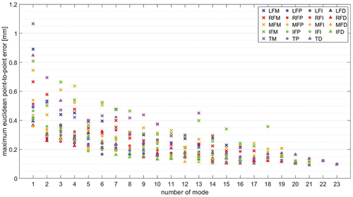
We observe maximal euclidean P2P surface distances below $1.07$ mm and 50% of all error values are below $0.22$ mm. Most prominent is the exponentially decaying influence of the modes on the surface error with increasing mode number. We will thus introduce weighted mode error metrics in Section 3.2 that weight the absolute error in each mode with the inverse of the mode’s number.

2.3. Reconstruction of 3D surface geometries

The description of 3D shapes through their SSM modes $\mathit{M}$ was explained in Section 2.2. For describing the position and orientation of the 3D shapes in space, we introduce a common orthogonal coordinate system that is placed in the centre of the SSM’s mean shape. Now, three translational components $\mathit{T}\in {\mathbb{R}}^3$ that describe the translations of the shape in $\mathit{x}$-, $\mathit{y}$-, and $\mathit{z}$-direction with respect to the common coordinate system are introduced. We describe the rotation of a 3D shape in space using unit quaternions $\mathit{q}=(q_x,q_y,q_z,q_w)$ with $||\mathit{q}||=1$. The three independent rotation components $q_x,q_y$, and $q_z$ are summarised in $\mathit{Q}$. Thus, the position and shape of a 3D bone is fully described by its SSM modes $\mathit{M}$, translation $\mathit{T}$, and rotation $\mathit{Q}$. If several input 2D X-ray images taken from different points of view are given, one set of transformation parameters $(\mathit{T},\mathit{Q}{)}^i$ describes the position of the 3D shape with respect to the $\mathit{i}$th input image. Note that the modes $\mathit{M}$, however, are the same for each projection direction. The proposed 3D shape reconstruction algorithm varies these parameters in each iteration and evaluates an objective function to estimate the quality of the selected parameters.

2.3.1. Objective function

Given a set of parameters $(\mathit{T},\mathit{Q},\mathit{M})$, we calculate the corresponding 3D shape using the SSM and modes $\mathit{M}$. The transformed shape is then projected onto a projection plane using orthographic projection. We call the nodes forming the outline of projected SSM mesh nodes $p_{\mathrm{p}}$ and the set of all such nodes $P_{\mathrm{p}}$.

A distance map $\mathit{D}$ is created from 2D reference bone outline images (synthetic data or contour segmentation of 2D X-rays). Given any spatial point on the 2D plane, the distance map returns the euclidean distance of that point to the reference contour of the depicted bone. We denote the set of all points $p_{\mathrm{o}}\in {\mathbb{R}}^2$ fulfilling $\mathit{D}(p_{\mathrm{o}})=0$ by $P_{\mathrm{o}}$.

There are two notions of distance, and thus two objective functions, implemented and compared in the present work. The objective function

(5) $F_1=\frac{||D({\mathit{P}}_{\mathrm{p}}{)||}_2}{|P_{\mathrm{p}}|}$(5)

evaluates the distance map at the points $p_{\mathrm{p}}\in P_{\mathrm{p}}$ and weighs it by the cardinality $|P_{\mathrm{p}}|$ of $P_{\mathrm{p}}$. The objective function

(6) $F_2=\frac{\sqrt{{\sum }_{{\mathit{p}}_{\mathrm{o}}\in P_{\mathrm{o}}}{min}_{{\mathit{p}}_{\mathrm{p}}\in P_{\mathrm{p}}}||p_{\mathrm{p}}-p_{\mathrm{o}}|{|}_2^2}}{|P_{\mathrm{o}}|}$(6)

calculates the distance of each point $p_o$ to the closest projected point $p_p$ and weighs it by $|P_{\mathrm{o}}|$.

If several input 2D X-ray images taken from different points of view are given, the corresponding transformation is applied to the 3D SSM geometry and the objective function is calculated for each input image. Finally, the objective function values for all input images are summed up. An additional regularisation term $\mathcal{W}(\mathit{M})$, which implements prior knowledge of the behaviour of the modes, can be added. The objective function then reads

(7) $\mathcal{F}(\mathit{T},\mathit{Q},\mathit{M})=\sum _i\left({\alpha }_F{F}_1((\mathit{T},\mathit{Q}{)}^i,\mathit{M})+(1-{\alpha }_F)F_2((\mathit{T},\mathit{Q}{)}^i,\mathit{M})\right)+{\alpha }_W\mathcal{W}(\mathit{M})$(7)

for a parameter ${\alpha }_F\in [0,1]$ balancing the influence of the two distance measures and a regularisation parameter ${\alpha }_W>0$. Four choices of regularisation terms have been analysed within this work:

• $W_1(\mathit{M}):=||\mathit{M}|{|}_1$ preferring small or few large modes,

• $W_2(\mathit{M}):=||\mathit{M}|{|}_2$ preferring small modes, especially modes smaller 1,

• $W_{\mathrm{\infty }}(\mathit{M}):=||\mathit{M}|{|}_{\mathrm{\infty }}$ punishing extreme values of the modes that are supposed to describe degenerated bones and should thus be rare,

• $W_{\mathrm{STD}}(\mathit{M}):=\frac{||M|{|}_2^2}{|\mathit{M}|}$ mimicking the behaviour of the underlying statistical model (compare to the computation of the STD).

2.3.2. Optimisation algorithm and parameters

The 2D-3D reconstruction minimising the objective function (7) is implemented using Matlab (MATLAB 2022). We use a bounded version of the Nelder-Mead simplex (direct search) method implemented in fminsearchbnd (D’Errico 2022). The maximum number of function evaluations was set to $500n_{\mathrm{M}}$ and the accuracy to ${10}^{-5}$. Optimisation of the transformation parameters and modes is done in three steps:

1. Find $\hat{T}=\underset{T\in {\mathrm{\Sigma }}_T}{arg\mathit{min}}\mathcal{F}(\mathit{T},\mathit{Q}=0,\mathit{M}=0)$ with admissible

   set ${\mathrm{\Sigma }}_T:=[-200,-200{]}^3$.

2. Find $(\tilde{T},\tilde{Q})=\underset{(\mathit{T},\mathit{Q})\in {\mathrm{\Sigma }}_{\mathit{TQ}}}{arg\mathit{min}}\mathcal{F}(\mathit{T},\mathit{Q},\mathit{M}=0)$ with admissible set ${\mathrm{\Sigma }}_{\mathit{TQ}}:=([\hat{T}-10,\hat{T}+10]\cap [-200,200{]}^3)\times [-1,1{]}^3$.

3. Find $(T^{\ast },Q^{\ast },M^{\ast })=\underset{(\mathit{T},\mathit{Q},\mathit{M})\in {\mathrm{\Sigma }}_{\mathit{TQM}}}{arg\mathit{min}}\mathcal{F}(\mathit{T},\mathit{Q},\mathit{M})$ with admissible set ${\Sigma }_{\mathit{TQ}}:={(\tilde{T}-10,\tilde{T}+10\cap -200,200]}^3\times {(\tilde{Q}-0.5,\tilde{Q}+0.5\cap -1,1]}^3\times {[-3,3]}^{n_{\text{M}}}$

We choose the starting values to be zeros for all parameters due to zero being the average value for each mode and due to the SSM coordinate system being centred in the origin. Free parameters are the parameters ${\alpha }_F$ and ${\alpha }_W$ introduced in Section 2.3.1, the choice of the regularisation term and the number of 2D images included in the optimisation process.

2.3.3. Generation of validation data sets

We use two data sets for validation. The first data set is a set of synthetic 2D bone contours. A random vector of modes $M^{\mathrm{ref}}$ being uniformly distributed in $[-1,1]$ is constructed. These modes are applied to the shape model of each finger. Additionally, known reference transformations are applied to the 3D bone shapes. Five reference transformations were adjusted:

VS0: no rotation, no translation

VS1: 30° rotation around the x-axis, $(5,13,29)$ mm translation in $(\mathit{x},\mathit{y},\mathit{z})$-direction

VS2: 30° rotation around the y-axis, $(5,13,29)$ mm translation in $(\mathit{x},\mathit{y},\mathit{z})$-direction

VS3: 30° rotation around the z-axis, $(5,13,29)$ mm translation in $(\mathit{x},\mathit{y},\mathit{z})$-direction

VS4: 30° rotation around the all 3 axes, $(5,13,29)$ mm translation in $(\mathit{x},\mathit{y},\mathit{z})$-direction

For generating synthetic 2D shapes, the computed 3D shape is projected to the xy-, xz- and yz-plane using orthographic projection. An image of the outline of the projected shape is then saved, representing the synthetic outline of a bone segmented in a 2D X-ray image. In the following, we will refer to these data as synthetic data. Note that we can include the knowledge about the orthogonality of the projection planes. Doing so reduces the number of free transformation parameters to the six parameters describing the orientation and position of the bone with respect to the known SSM coordinate system.

The second validation data set is generated from CT scans of 35 patients, where additional X-ray images of the fingers were taken. For each finger bone, the corresponding SSM was fitted to the 3D voxel mask obtained from the segmented CT images (3D-3D-fitting). The resulting SSM modes were saved as reference solution. Further, the fitted SSM and the original CT geometry were saved for P2P error estimation. 2D shapes of the finger bones were generated from the segmented X-ray images and served as input for the 2D-3D reconstruction described in Section 3.3

3. Results

3.1. SSM accuracy

A leave-one-out cross-validation (LOOCV) is performed on the shape model data for evaluating the SSM accuracy. Therefore, an SSM is build from all but one shapes. The resulting SSM is fitted to the remaining shape and the accuracy is measured. This process is repeated until each shape was fitted once. We perform the LOOCV on SSM75 and SSM95 for each bone. Figures 2 and 3 show box plots of the computed mean surface distances for both SSMs.

Figure 2. Average surface distance of fitted SSM to original 3D mask accounting for 75% of the shape variance.

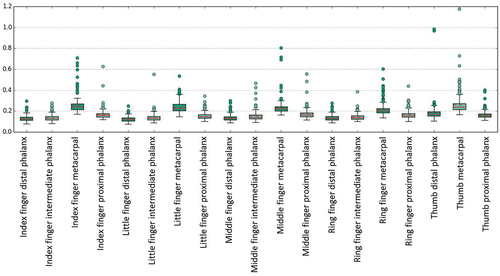
Figure 3. Average surface distance of fitted SSM to original 3D mask accounting for 95% of the shape variance.

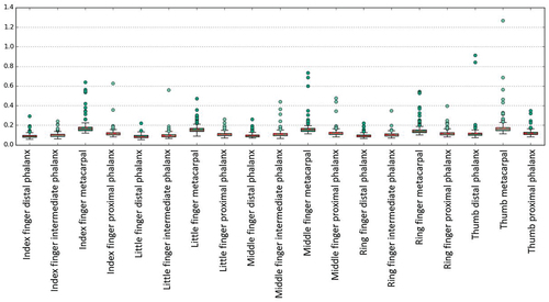
We see that both SSM variants show similar behaviour. However, the results for SSM95 show a slightly lower average error and a more prominent outlier value for the thumb metacarpal phalanx. Most errors and outliers are visible for the metacarpal bones. Averaged across all bones, the average mean distance between shape model reconstruction and segmentation mask is $\approx 0.1$ mm for SSM95 and $\approx 0.2$ mm for SSM75. The average maximum distance between shape model reconstruction and segmentation mask is $\approx 0.4$ mm ($\approx 0.5$ mm for metacarpal bones) for SSM95 and $\approx 0.5$ mm ($\approx 0.6$ mm for metacarpal bones) for SSM75. Summarising, both SSMs show high accuracy in representing unknown shapes. Going from SSM75 to SSM95, the gain in terms of accuracy is small while the number of modes and thus free optimisation parameters is more than quadrupled. With regard to the optimisation process, using SSM75 is clearly preferable since it balances performance and accuracy.

3.2. Proof of concept

We ran several parameter studies on the synthetic data described in Section 2.3.3 for calibration of the free optimisation parameters. These are the distance metric weighting parameter ${\alpha }_F$, the regularisation parameter ${\alpha }_W$, the regularisation term $\mathcal{W}$, and the number of input X-ray images/projection directions. The parameter study was conducted for all five reference configurations VS0-VS4 for each finger bone (metacarpal, proximal, intermediate and distal phalanx of little, ring, middle, and index finger and metacarpal, proximal, and distal phalanx of the thumb) using two orthogonal projection directions.

We introduce the following error norms for evaluation of the results:

• The euclidean distance $||\cdot |{|}_2$, e.g. for comparison of translations in 3D.

• The mean and maximum euclidean P2P error $||P^{\ast }-P^{\mathrm{ref}}|{|}_{2,-}$ and $||P^{\ast }-P^{\mathrm{ref}}|{|}_{2,\mathrm{\infty }}$ measuring the mean and maximum euclidean distance between corresponding computed and reference points $P^{\ast }$ and $P^{\mathrm{ref}}$.

• The Haussdorf surface distance

  $d_{\mathrm{H}}(P^{\ast },P^{\mathrm{ref}})=max\{\underset{p^{\ast }\in P^{\ast }}{sup}\underset{{\mathit{p}}^{\mathrm{ref}}\in P^{\mathrm{ref}}}{inf}(p^{\ast },p^{\mathrm{ref}}),\underset{{\mathit{p}}^{\mathrm{ref}}\in P^{\mathrm{ref}}}{sup}\underset{p^{\ast }\in P^{\ast }}{inf}(p^{\ast },p^{\mathrm{ref}})\}.$

• The mean and maximum weighted absolute modes error

  $d_{\mathrm{M},-}(M^{\ast },M^{\mathrm{ref}})\frac{1}{{\mathit{n}}_{\mathrm{M}}}\sum _{\mathit{i}=1}^{{\mathit{n}}_{\mathrm{M}}}\frac{|M_i^{\ast }-M_i^{\mathrm{r}\mathrm{e}\mathrm{f}}|}{\mathit{i}}\mathrm{and}$
  $d_{\mathrm{M},\mathrm{\infty }}(M^{\ast },M^{\mathrm{ref}})\underset{\mathit{i}=1,\dots ,{\mathit{n}}_{\mathrm{M}}}{max}\frac{|M_i^{\ast }-M_i^{\mathrm{r}\mathrm{e}\mathrm{f}}|}{\mathit{i}}.$

We define spatial differences below 1 mm and rotational differences below 5° to be acceptable for clinical applications.

3.2.1. Balancing the distance metrics

The parameter ${\alpha }_F$ balances the two distance metrics introduced in Equations (5)(5) $F_1=\frac{||D({\mathit{P}}_{\mathrm{p}}{)||}_2}{|P_{\mathrm{p}}|}$(5) and (6(6) $F_2=\frac{\sqrt{{\sum }_{{\mathit{p}}_{\mathrm{o}}\in P_{\mathrm{o}}}{min}_{{\mathit{p}}_{\mathrm{p}}\in P_{\mathrm{p}}}||p_{\mathrm{p}}-p_{\mathrm{o}}|{|}_2^2}}{|P_{\mathrm{o}}|}$(6) ). We vary ${\alpha }_F\in \left\{0,0.1,0.3,0.5,0.7,0.9,1\right\}$ and set the regularisation parameter ${\alpha }_W=0$. Figure 4 summarises the statistics of the different error metrics for the parameter study for investigating the influence of the parameter ${\alpha }_F$. Note that semi-logarithmic plots were used to emphasize the behaviour of the majority of data points in contrast to the few outliers. To better visualise outlier distributions and values, the upper 5% of all values are plotted individually.

Figure 4. Statistics summarising different error metrics of all bones and reference configurations VS0-VS4 for ${\alpha }_F\in \{0,0.1,0.3,0.5,0.7,0.9,1\}$ and ${\alpha }_W=0$.

Most prominently, the mean and median values are clearly separated due to the few but large outlier values. Looking at the majority of the error values, 75% of all values are below 4° for the rotational error and below 0.2 mm for the translational error. This results in less then 0.4 mm mean euclidean P2P difference and less then 0.9 mm maximum euclidean P2P difference (0.8 mm Hausdorff distance). The exact numerical values can be found in Table A1 in the Appendix. Here, also the statistical values for the mode errors and Hausdorff surface distances are included. The modes error norms are, however, similar for each value of ${\alpha }_F$ and will be investigated in detail when regularisation is incorporated.

The number of outlier values not fulfilling the criterion defined in Section 3.2 for the respective error metrics are summarised in Table 1.

Table 1. Number of outlier error values larger than 5° for rotation errors and 1 mm for translation and surface error metrics among 2D-3D reconstructions of all bones and reference configurations VS0-VS4 for ${\alpha }_F\in \{0,0.1,0.3,0.5,0.7,0.9,1\}$ and ${\alpha }_W=0$.

${\alpha }_F$	0	0.1	0.3	0.5	0.7	0.9	1
# rotation error $>5$	20	10	13	13	15	10	11
# $||T^{\ast }-T^{\mathrm{ref}}|{|}_2>1$ mm	3	2	2	1	3	2	2
# $||P^{\ast }-P^{\mathrm{ref}}|{|}_{2,-}>1$ mm	8	4	4	6	7	5	7
# $||P^{\ast }-P^{\mathrm{ref}}|{|}_{2,\mathrm{\infty }}>1$ mm	17	11	13	12	11	10	11
# $d_{\mathrm{H}}(P^{\ast },P^{\mathrm{ref}})>1$ mm	16	10	13	11	11	10	10
total number of outliers	64	37	45	43	47	37	41

Most outliers and the highest statistical values, see Figure 4, are observable for ${\alpha }_F=0$. The statistical values for ${\alpha }_F\in \{0.1,0.3,0.5,0.7,0.9,1\}$ show only smaller variations. However, for ${\alpha }_F=0.1$ the rotation error is below 7.5° for 95% of all computed examples, while the other rotation error 95th percentile values are in the range between 10° and 20°. Consequently, the geometric error metrics (mean and max P2P error, Hausdorff surface distance) are also lowest for ${\alpha }_F=0.1$. Contrarily, the mean and maximum weighted modes error are lowest for ${\alpha }_F=0.9$.

We fix ${\alpha }_F=0.1$ and further fine-tune the influence and fitting of the modes by analysing the influence of the regularisation parameter and term.

3.2.2. Choosing the regularisation parameter

For this parameter study, we use the objective function $\mathcal{F}=0.1F_1+0.9F_2+{\alpha }_W\mathcal{W}$ with regularisation term $\mathcal{W}\in \{W_1,W_2,W_{\mathrm{\infty }},W_{\mathrm{STD}}\}$ and regularisation parameter ${\alpha }_W\in \{0.01,0.05,0.1,0.5,1,5\}$. Figure 5 summarises the statistics of that parameter study, highlighting the influence of the regularisation parameter.

Figure 5. Statistics summarising different error metrics of all bones and reference configurations VS0-VS4 for distance measure $\mathcal{F}=0.1F_1+0.9F_2+{\alpha }_W\mathcal{W}$ with ${\alpha }_W\in \{0,0.01,0.05,0.1,0.5,1,5\}$, $\mathcal{W}\in \{W_1,W_2,W_{\mathrm{\infty }},W_{\mathrm{STD}}\}$.

Most prominently, regularisation seams to increase the modes and P2P error measures. Translational and rotational components are barely influenced by the modes regularisation and plots are thus neglected here. Further, the modes error metrics increase with increasing regularisation parameter ${\alpha }_W$. Recall that the presented error plots also accumulate the errors for all proposed regularisation terms. We conclude that choosing small regularisation parameters seams to be most appropriate, fix ${\alpha }_W=0.01$, and further investigate the influence of regularisation in the following.

3.2.3. Choosing the regularisation term

For $\mathcal{F}=0.1F_1+0.9F_2+0.01\mathcal{W}$ we investigate the influence of the regularisation term $\mathcal{W}\in \{W_1,W_2,W_{\mathrm{\infty }},W_{\mathrm{STD}}\}$ compared to the non-regularisation setting $\mathcal{W}=\mathrm{none}$. The results are shown in Figure 6.

Figure 6. Statistics summarising different error metrics of all bones and all five reference configurations VS0-VS4 for distance measure $\mathcal{F}=0.1F_1+0.9F_2+0.01\mathcal{W}$ with $\mathcal{W}\in \{\mathrm{none},W_1,W_2,W_{\mathrm{\infty }},W_{\mathrm{STD}}\}$.

As before, we see increase in error metrics using regularisation except for regularisation terms $W_2$ and $W_{\mathrm{\infty }}$. The median and mean values are, however, similar and, more prominent, a slight decrease in the 95th percentiles for all error metrics is visible. This decrease of the 95th percentile also influences the number of outliers as defined in Section 3.2, see Table 2.

Table 2. Number of outlier error values larger than 5° for rotation errors and 1 mm for translation and surface error metrics among 2D-3D reconstructions of all bones and reference configurations VS0-VS4 for distance measure $\mathcal{F}=0.1F_1+0.9F_2+0.01\mathcal{W}$ with $\mathcal{W}\in \{\mathrm{none},W_1,W_2,W_{\mathrm{\infty }},W_{\mathrm{STD}}\}$.

$\mathcal{W}$	none	$W_1$	$W_2$	$W_{\mathrm{\infty }}$	$W_{\mathrm{STD}}$
# angle error $>5$°	10	15	8	8	10
# $||T^{\ast }-T^{\mathrm{ref}}|{|}_2>1$ mm	2	2	2	2	2
# $||P^{\ast }-P^{\mathrm{ref}}|{|}_{2,-}>1$ mm	4	6	3	2	4
# $||P^{\ast }-P^{\mathrm{ref}}|{|}_{2,\mathrm{\infty }}>1$ mm	11	15	9	8	9
# $d_{\mathrm{H}}(P^{\ast },P^{\mathrm{ref}})>1$ mm	10	14	9	7	9
total number of outliers	37	52	31	27	34

While 1-norm regularisation clearly impairs the number of outliers, all other regularisation terms decrease the number of outliers. Lowest total number of outliers is achieved using $W_{\mathrm{\infty }}$. More precisely, outliers are observed for reference configuration VS0 for index finger distal (VS0-IFD), VS1 for index finger metacarpal (VS1-IFM), VS2 for thumb metacarpal (VS2-TM), VS3 for little and ring finger metacarpal (VS3-LFM, -RFM), VS4 for ring finger proximal (VS4-RFP) and middle finger, index finger, and thumb metacarpal (VS4-MFM, -IFM, -TM). Hence, seven out of nine outliers are caused by metacarpal bones. While one of the outliers produces an optically good fit (see Figure 7a), the optical fit of most outliers looks only good in the two used projection directions and show differences in the third projection direction, see Figure 7b for an example. Two of the outliers even produce clearly visible mismatches in the first two projection directions, see Figure 7c for an example. We investigate the potential of improving the matching results for these outliers by using an additional third projection direction in the following section.

Figure 7. Black: reference synthetic X-ray/SSM mesh, orange: projection of fitted SSM.

3.2.4. Choosing the number of projection directions

For investigating the influence of the number of projection directions, we do the 2D-3D reconstruction for all five reference configurations and all finger bones comparing one projection direction vs two (perpendicular) projection directions vs three (perpendicular) projection directions. We use the projection in $\mathit{x}$-direction in the one projection case, projections in $\mathit{x}$- and $\mathit{y}$-directions in the two projections case and projections in $\mathit{x}$-, $\mathit{y}$-, and $\mathit{z}$-directions in the three projections case. Figure 8 summarises the different error metrics for the parameter study using the objective function $\mathcal{F}=0.1F_1+0.9F_2+0.01W_{\mathrm{\infty }}$.

Figure 8. Statistics summarising different error metrics of all bones and all five reference configurations VS0-VS4 for distance measure $\mathcal{F}=0.1F_1+0.9F_2+0.01W_{\mathrm{\infty }}$ using one, two and three projection directions.

Using only one projection direction, the distance between projection and projected object (using orthographic projection) is not well defined. We thus see high translational and P2P errors. Hence, rotation and SSM mode detection is less accurate. Including a second projection direction helps locating the SSM in space and thus improves translational and P2P error as well as rotation and modes error significantly. Contrarily, including a third projection direction only leads to minor improvements in mean and median error metrics, while outlier values and 95th percentile often become worse. The overall computation time and number of outliers, as defined in Section 3.2, for one, two, and three projection directions shown in Table 3 underline this behaviour.

Table 3. Computation time accumulated for all 2D-3D reconstructions and number of outlier error values larger than 5° for rotation errors and 1 mm for translation and surface error metrics among 2D-3D reconstructions of all bones and reference configurations VS0-VS4 for distance measure $\mathcal{F}=0.1F_1+0.9F_2+0.01W_{\mathrm{\infty }}$ using one, two and three projection directions.

# projection directions	1	2	3
computation time [h]	3:34	7:28	9:34
# angle error $>5$°	41	8	8
# $||T^{\ast }-T^{\mathrm{ref}}|{|}_2>1$ mm	95	2	1
# $||P^{\ast }-P^{\mathrm{ref}}|{|}_{2,-}>1$ mm	95	2	2
# $||P^{\ast }-P^{\mathrm{ref}}|{|}_{2,\mathrm{\infty }}>1$ mm	95	8	9
# $d_{\mathrm{H}}(P^{\ast },P^{\mathrm{ref}})>1$ mm	95	7	8
total number of outliers	421	27	28

We see that the number of outliers is nearly unchanged when introducing a third projection direction, while the overall computation times increases linearly with the number of projection directions used. Nevertheless, looking at the outliers produced by using only two projection directions, Table 4 shows great improvement including a third projection direction for seven out of nine cases.

Table 4. Comparison of different error metrics of outliers using two vs. three projection directions (PD) for distance measure $\mathcal{F}=0.1F_1+0.9F_2+0.01W_{\mathrm{\infty }}$.

	rotation error [°]		$||T^{\ast }-T^{\mathrm{ref}}|{|}_2$ [mm]		$||P^{\ast }-P^{\mathrm{ref}}|{|}_{2,\mathrm{\infty }}$ [mm]
outlier	2 PD	3 PD	2 PD	3 PD	2 PD	3 PD
VS0-IFD	5.41	0.60	0.07	0.01	0.59	0.25
VS1-IFM	5.08	0.75	0.18	0.15	1.37	0.46
VS2-TM	7.85	4.92	0.32	0.27	1.82	1.19
VS3-LFM	7.59	3.30	0.37	0.14	1.32	0.75
VS3-RFM	8.70	9.54	0.19	0.24	1.52	2.31
VS4-RFP	5.36	1.24	0.20	0.09	1.38	0.54
VS4-MFM	3.32	1.90	0.07	0.06	1.04	0.53
VS4-IFM	36.73	43.67	1.45	1.17	7.51	8.19
VS4-TM	33.13	0.40	1.31	0.09	6.41	0.30

Summarising the above findings and weighting computation time and accuracy, we find that using two projection directions is sufficient in most cases in terms of 2D-3D reconstruction accuracy. The error metrics are summarized in Table A2 in the appendix. In terms of obvious discrepancies between X-ray and projected contour, including a third projection direction is likely to improve the results. Outlier handling is further discussed in Section 4.

3.2.5. Summary of optimisation parameters

Summarising the above findings, we have $\mathcal{F}=0.1F_1+0.9F_2+0.01W_{\mathrm{\infty }}$ using two projection directions as the best parameter combination for 3D shape reconstruction on the synthetic datA. The statistical error values for this configuration are summarised in Table 2. We reach high accuracy for 95% of all data points: rotational error $<5.75$° (7.5° without regularisation), maximal euclidean P2P surface error and Hausdorff surface distance $<1.37$ mm (1.88 mm without regularisation). Moreover, only 8.42% of the data points do not fulfill our restrictive quality constraints on the rotation and maximum P2P error.

3.3. Application to real data

We apply the 2D-3D reconstruction using the objective function $\mathcal{F}=0.1F_1+0.9F_2+0.01W_{\mathrm{\infty }}$ to the real data described in Section 2.3.3. Note that the true positioning and orientation of the X-ray images with respect to the CT data is unknown. Thus, the evaluation of these experiments will not contain error measurements concerning the translational and rotational components. Further, the X-ray images are no longer orthogonal. Therefore, three rotational and three translational parameters need to be computed for each X-ray image. Moreover, we emphasize that a single ground truth does not exist when segmenting medical image data, since segmentations show high inter- and intra-observer variability (Menze et al. 2015; Joskowicz et al. 2018). For evaluating the quality of the 2D-3D reconstruction, we introduce the following error measures:

• Hausdorff distance $d_{\mathrm{H}}(P^{\mathrm{ref}},P^{\mathrm{CT}})$ between 3D-3D-fitted SSM and original CT (SSM 3D-3D fitting accuracy + CT segmentation error)

• Hausdorff distance $d_{\mathrm{H}}(P^{\ast },P^{\mathrm{CT}})$ between 2D-3D-fitted SSM and original CT

• mean and maximum P2P error between 2D-3D-fitted SSM and original CT

• Hausdorff distance $d_{\mathrm{H}}(P^{\ast },P^{\mathrm{ref}})$ between 2D-3D-fitted and 3D-3D-fitted SSM (SSM 2D-3D fitting accuracy + X-ray segmentation error)

• mean and maximum P2P error between 2D-3D-fitted and 3D-3D-fitted SSM

• mean and maximum weighted modes error $d_{\mathrm{M},-}(M^{\ast },M^{\mathrm{ref}})$ and $d_{\mathrm{M},\mathrm{\infty }}(M^{\ast },M^{\mathrm{ref}})$

Figure 9a summarises the introduced error metrics for all 34 patients and finger bones. The numerical data are shown in Table A3 in the appendix.

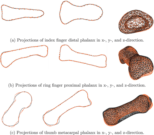
Figure 9. 2D-3D reconstruction with distance measure $\mathcal{F}=0.1F_1+0.9F_2+0.01W_{\mathrm{\infty }}$ for real data.

Generally, the surface distance errors are approximately twice as high as for the synthetic data set. While the Hausdorff and the maximum euclidean P2P surface distances are below 1 mm for 75% of all synthetic data, the Hausdorff and the maximum euclidean P2P surface distances between the 2D-3D-fitted SSM and the original CT are only below 2 mm for 75% of all real datA. The maximum euclidean P2P surface distances between the 2D-3D-fitted SSM and the original CT are below 3.32 mm for 95% of all real data with a maximum difference of 6.86 mm. The mean and median values of these distance measures are about 1.5 mm. The 3D-3D-reconstruction error that is zero for the synthetic data set is below 1 mm for 82.11% of all cases and below 2 mm for 99.55% of all cases. We emphasize that during 2D-3D reconstruction, 2D segmentation error, 2D-3D reconstruction error, SSM accuracy, and 3D segmentation error accumulate. However, adding the Hausdorff surface distance between 2D-3D-fitted SSM and 3D-3D-fitted SSM to the Hausdorff surface distance between 3D-3D-fitted SSM and original CT yields a strict upper bound for the Hausdorff surface distance between 2D-3D-fitted SSM and original CT, i.e. the accumulated error is lower than the sum of its components.

Figure 9b shows the Hausdorff surface distance between 2D-3D-fitted SSM and original CT summarised for each bone. For each finger, the Hausdorff surface distance decreases from proximal to distal, similar to the SSM accuracy results in Section 3.1.

4. Discussion

We introduced and validated a method for reconstructing 3D finger bone shapes from 2D X-ray scans of those bones with the help of SSMs. The information that can be added to 2D imaging by 2D-3D reconstruction is manifold. Examples are 3D motion modelling and the 3D axis computation of anatomical structures. The additional 3D information has high potential to improve diagnosis and therapy. Furthermore, the advantages of using (few) X-ray images compared to one CT or MRI scan are numerous. Compared to a full CT scan, there is the reduction of radiation dose for patients and clinicians. Moreover, X-ray imaging modalities are available more frequently. Thus, using X-ray scans instead of CT or MRI helps accelerating the process from first contact to a physician to diagnosis and treatment. Further, costs are reduced for patients and insurances.

Evaluating the proposed method on the synthetic data set, 91.58% of all patients could benefit from our method, assuming that the defined accuracy of 1 mm is sufficient. Applying the method to real data, the X-ray projection directions are no longer orthogonal. Worse, in most patients, they only differ slightly such that the amount of additional information contained in the second scan can be assumed to be relatively small. A comparison of the results for synthetic and real data indicates that using more orthogonal projection directions might improve the reconstruction results. However, segmentation is difficult for human and AI in X-ray images taken in sagittal direction due to the bones shadowing each other. Nevertheless, high-quality segmentations are essential for performing accurate 2D-3D reconstruction. In the presented real data, segmentations of metacarpal bones are the most error prone since they are most frequently affected by shadowing either from neighbouring metacarpal or wrist bones. Moreover, segmentation errors in both, 2D and 3D images, influence the SSM quality and fitting ability. Figure 9b shows that errors in reconstructing the metacarpal bones are significantly higher than for other bones, which supports our theory.

The achieved 2D-3D reconstruction errors are within the same range as those published for reconstruction of different bones: For the reconstruction of the rib cage from two orthogonal x-ray images (Dworzak et al. 2009), reached reconstruction errors in the range of 2.2 to 4.7 mm for the average mean 3D surface distance. In (Baka et al. 2011) root mean squared point-to-surface distances between 0.68 mm and 1.68 mm were achieved reconstructing the 3D shape of the distal femur from biplane fluoroscopic images. The 3D shape of the radius and ulna could be reconstructed with accuracies of $1.34\pm 0.39$ mm and $1.64\pm 0.39$ mm in (Shiode et al. 2021).

For application in clinical routine, outliers and uncertainties will have to be quantified. One possibility for outlier detection is to display the objective function value either in numbers or converted to a green (most likely acceptable accuracy) to red (most likely not sufficiently accurate) colour scale. Additionally, the projections of the reconstructed shape into the x-ray images can be displayed to the clinician and evaluated manually. Visualising the intersection of the two x-ray images may also yield a simple sanity check. In addition, including another X-ray image from a third projection direction into the 2D-3D reconstruction procedure can be recommended when uncertainties are below a defined threshold. A third projection direction can reduce the errors in many cases, as seen in Section 3.2.4.

Applicability of the algorithm to other structures, e.g. the pelvis or knee, and more advanced use cases, e.g. dealing with fractures/missing information, has to be investigated in future work.

5. Conclusion

We introduced a method for fitting 3D shapes from two 2D X-ray images, adding precious 3D information to 2D imaging and eliminating the need for expensive 3D imaging in other cases. The influence of the method parameters on the 2D-3D reconstruction of finger bones was extensively validated on a synthetic data set. 2D-3D reconstruction results of that parameter study showed the high reconstruction ability of the proposed method. Further validation was done on 34 patient data sets of corresponding X-ray and CT images. In contrast to other approaches, the two X-ray projection directions are not perpendicular for those patients.

For synthetic data, 91.58% of all cases show surface errors below 1 mm. For real data, 79.65% of all cases show surface errors below 2 mm, while 23.31% are below 1 mm. For application of the method in clinical routine, uncertainties have to be quantified, displayed and performing additional X-ray or CT/MRI scans should be recommended in case of high uncertainty.

Apart from finger bone shape reconstruction, the proposed method can be applied to any structure, e.g. the femur, pelvis, or teeth. Further extensions to fractured bone or otherwise missing shape information can easily be included. Concluding, the proposed method opens the opportunity to do 3D surgery planning, construction of individual implants, or physiological motion modelling without acquiring cost, time (and radiation) expensive 3D images.

Disclosure statement

No potential conflict of interest was reported by the author(s).

Additional information

Funding

This work was supported by the Fraunhofer Internal Programs under Grant [No. PREPARE 840226].

Notes on contributors

Anna Rörich

Anna Rörich did her BSc and MSc in Applied Mathematics from the Technical University of Dortmund, Germany and received her doctoral degree from the University of Stuttgart, Germany. For her thesis, she worked on parameter identification from electromyographic signals. Since 2021 she is with Fraunhofer Institute for Digital Medicine MEVIS. She works on 2D-3D shape reconstruction and modelling and simulation in the orthopaedic field.

Annkristin Lange

Annkristin Lange, MSc (female) has been a member of the image registration group at the Fraunhofer Institute for Digital Medicine MEVIS for about 5 years. As an applied mathematician in the field of imaging, she has a sound background in the development and analysis of algorithms for medical image processing. Her expertise is in statistical shape modelling and image registration of pre-interventional CT and intra-interventional X-rays.

Stefan Heldmann

Stefan Heldmann studied computer science and medical informatics and received his doctoral degree in 2006 from the University of Lübeck, Germany. From 2005 to 2007, he worked as a postdoc at the Department of Mathematics and Computer Science at Emory University, Atlanta, GA, USA, before returning to Lübeck as a research associate at the Institute of Mathematics and joining Fraunhofer MEVIS in 2009, where he is currently Head of Image Registration. He has over 15 years of research experience focusing on image registration for practical applications with special interest in numerical methods, inverse problems, optimization and implementation aspects.

Jan H. Moltz

Jan H. Moltz studied computer science at the University of Lübeck, Germany and obtained a PhD from Jacobs University Bremen, Germany in 2013. He has been a research engineer at Fraunhofer MEVIS, Bremen, Germany since 2006 and is currently leading a group that develops solutions for efficient CT-based tumor follow-up. He has been working on medical image segmentation and analysis for a wide range of clinical applications.

Lars Walczak

Lars Walczak is a German computer scientist and post-doctoral researcher. He holds a diploma degree in computer science and received his doctorate in natural sciences in 2016 with a thesis on computational hemodynamic modelling in aneurysms, both awarded from TU Dortmund University in Germany. For ten years, he was a researcher at the Chair for Computer Graphics at TU Dortmund University. In 2018, he joined Fraunhofer Institute for Digital Medicine MEVIS as a Senior Scientist. Since 2018, he is also affiliated with Charité – Universitätsmedizin Berlin, Deutsches Herzzentrum der Charité (DHZC), Institute for Computer-assisted Cardiovascular Medicine, Berlin, Germany.

Sinef Yarar-Schlickewei

Sinef Yarar-Schlickewei, MD, is a senior physician in the Department of Trauma Surgery and Orthopedics at the University Medical Center Hamburg-Eppendorf. The study of human medicine and the specialist training was carried out at the University Medical Center Hamburg-Eppendorf. In 2002 she was licensed as a physician and in 2009 as a specialist in trauma surgery and orthopedics. Moreover, she holds the additional designations for hand surgery (FESSH) and special trauma surgery. Her clinical and research focus is hand surgery in addition to trauma surgery.

Felix Güttler

Felix Güttler did his Diploma in Computer Science at the Free University of Berlin in collaboration with the Fraunhofer Institute for Open Communication Systems (FOKUS) in 2007. Subsequently, he became research associate at the Charité - Universitätsmedizin Berlin in the field of computer vision in interventional radiology. Later he became speaker and project leader for OMRT. Since 2012 he is scientifically active at the University Hospital Jena as working group leader in translational research and later became commercial-technical director of the Institute for Diagnostic and Interventional Radiology.

Joachim Georgii

Joachim Georgii is Key Scientist for modeling and simulation at Fraunhofer MEVIS, Bremen. From 2007 to 2010, he was a PostDoc at the computer graphics and visualization group at the Technische Universität München. In 2007, Joachim Georgii received a doctoral degree from the Technische Universität München. In 2003 he received a diploma in computer science. He has 20 years on research experience focusing on physics-based simulation, deformation, geometric methods as well as their efficient implementation using parallelization and concurrency on multi- and manycore architectures. His research supports medical applications ranging from image-guided treatment planning to medical image analysis.

A.

Statistical data

Table A1. Error statistics of all bones and reference configurations VS0-VS4 for ${\alpha }_F\in \{0,0.1,0.3,0.5,0.7,0.9,1\}$ and ${\alpha }_W=0$.

${\alpha }_F$		0	0.1	0.3	0.5	0.7	0.9	1
rotational error [°]	mean	4.48	2.97	3.17	3.14	3.62	3.13	3.21
	median	1.99	1.50	1.42	1.49	1.68	1.59	1.52
	75th percentile	3.76	3.02	3.56	3.11	3.20	2.90	3.16
	95th percentile	18.56	7.50	9.22	12.71	13.86	14.42	13.85
	maximum	53.54	46.38	34.94	34.77	35.20	35.59	33.82
$||T^{\ast }-T^{\mathrm{ref}}|{|}_2$ [mm]	mean	0.16	0.12	0.12	0.11	0.13	0.12	0.13
	median	0.08	0.07	0.07	0.06	0.06	0.07	0.06
	75th percentile	0.14	0.13	0.13	0.12	0.12	0.13	0.11
	95th percentile	0.47	0.27	0.31	0.41	0.43	0.27	0.32
	maximum	1.71	1.64	1.44	1.27	1.39	1.49	1.31
$d_{\mathit{M},\mathrm{\infty }}(\mathit{M}{,}^{\ast }{M}^{\mathrm{ref}})$ [STD]	mean	0.25	0.21	0.20	0.19	0.20	0.18	0.18
	median	0.18	0.19	0.18	0.16	0.16	0.14	0.14
	75th percentile	0.30	0.26	0.25	0.21	0.25	0.22	0.21
	95th percentile	0.53	0.49	0.47	0.42	0.55	0.39	0.43
	maximum	1.66	0.62	0.93	1.05	1.20	1.01	1.05
$||P^{\ast }-P^{\mathrm{ref}}|{|}_{2,-}$ [mm]	mean	0.48	0.36	0.36	0.34	0.39	0.34	0.35
	median	0.24	0.19	0.19	0.19	0.21	0.18	0.20
	75th percentile	0.36	0.31	0.31	0.31	0.30	0.29	0.31
	95th percentile	1.20	0.79	0.91	1.06	1.39	0.96	1.39
	maximum	4.78	4.95	3.84	3.67	4.32	3.77	3.62
$||P^{\ast }-P^{\mathrm{ref}}|{|}_{2,\mathrm{\infty }}$ [mm]	mean	0.97	0.75	0.74	0.69	0.79	0.72	0.73
	median	0.52	0.43	0.43	0.44	0.44	0.40	0.42
	75th percentile	0.81	0.71	0.68	0.69	0.65	0.62	0.71
	95th percentile	2.65	1.88	1.85	2.03	2.89	2.09	2.93
	maximum	8.73	9.66	7.80	7.20	7.62	7.51	7.28
$d_{\mathrm{H}}(P^{\ast },P^{\mathrm{ref}})$ [mm]	mean	0.75	0.65	0.62	0.59	0.63	0.59	0.60
	median	0.52	0.43	0.43	0.44	0.44	0.40	0.42
	75th percentile	0.79	0.69	0.68	0.69	0.65	0.62	0.71
	95th percentile	1.88	1.56	1.45	1.59	1.82	1.48	1.68
	maximum	4.18	5.72	4.35	3.85	4.44	4.19	3.51

Table A2. Error statistics of all bones and reference configurations VS0-VS4 for $\mathcal{F}=0.1F_1+0.9F_2+0.01W_{\mathrm{\infty }}$ using two projection directions.

	mean	median	75th percentile	95th percentile	maximum
rotation error [°]	2.69	1.37	3.17	5.75	36.73
$||T^{\ast }-T^{\mathrm{ref}}|{|}_2$ [mm]	0.12	0.07	0.12	0.21	1.45
$d_{\mathrm{M},-}(M^{\ast },M^{\mathrm{ref}})$ [STD]	0.05	0.05	0.06	0.07	0.12
$d_{\mathrm{M},\mathrm{\infty }}(M^{\ast },M^{\mathrm{ref}})$ [STD]	0.23	0.22	0.29	0.40	0.63
$||P^{\ast }-P^{\mathrm{ref}}|{|}_{2,-}$ [mm]	0.33	0.21	0.31	0.63	4.00
$||P^{\ast }-P^{\mathrm{ref}}|{|}_{2,\mathrm{\infty }}$ [mm]	0.68	0.47	0.65	1.37	7.51
$d_{\mathrm{H}}(P^{\ast },P^{\mathrm{ref}})$ [mm]	0.60	0.47	0.65	1.27	4.63

Table A3. Error statistics for real data 2D-3D reconstruction.

	mean	median	75th percentile	95th percentile	maximum
$d_{\mathrm{H}}(P^{\mathrm{ref}},P^{\mathrm{CT}})$ [mm]	0.79	0.72	0.92	1.29	3.05
$d_{\mathrm{H}}(P^{\ast },P^{\mathrm{CT}})$ [mm]	1.58	1.33	1.85	3.16	6.43
$||P^{\ast }-P^{\mathrm{CT}}|{|}_{2,-}$ [mm]	0.61	0.55	0.71	1.13	2.74
$||P^{\ast }-P^{\mathrm{CT}}|{|}_{2,\mathrm{\infty }}$ [mm]	1.64	1.39	1.92	3.32	6.86
$d_H(P^{\ast },P^{\mathrm{ref}})$ [mm]	1.32	1.09	1.53	2.86	5.64
$||P^{\ast }-P^{\mathrm{ref}}|{|}_{2,-}$ [mm]	0.53	0.46	0.64	1.01	1.65
$||P^{\ast }-P^{\mathrm{ref}}|{|}_{2,\mathrm{\infty }}$ [mm]	1.34	1.09	1.54	3.05	5.65
$d_{\mathit{M},-}(M^{\ast },M^{\mathrm{ref}})$ [STD]	0.17	0.15	0.21	0.31	0.50
$d_{\mathit{M},\mathrm{\infty }}(M^{\ast },M^{\mathrm{ref}})$ [STD]	0.91	0.76	1.19	1.97	3.48

References

- Amiranashvili T, Lüdke D, Li H, Menze B, Zachow S. 2022. Learning shape reconstruction from sparse measurements with neural implicit functions. Proceedings of Machine Learning Research; Zürich.
- Baka N, Kaptein B, de Bruijne M, van Walsum T, Giphart J, Niessen W, Lelieveldt B. 2011. 2d–3d shape reconstruction of the distal femur from stereo x-ray imaging using statistical shape models. Med Image Anal. 15(6):840–15.
- Cresson T, Branchaud D, Chav R, Godbout B, de Guise J. 2010. 3d shape reconstruction of bone from two x-ray images using 2d/3d nonrigid registration based on moving least-squares deformation. Progress in Biomedical Optics and Imaging - Proceedings of SPIE; San Diego, California, United States; Vol. 7623. p. 03.
- D’Errico J. fminsearchbnd, fminsearchcon. MATLAB Central File Exchange. [accessed 23 Feb 2022]. https://www.mathworks.com/matlabcentral/fileexchange/8277-fminsearchbnd-fminsearchcon.
- Dworzak J, Lamecker H, von Berg J, Klinder T, Lorenz C, Kainmüller D, Seim H, Hege H-C, Zachow S. 2009. 3d reconstruction of the human rib cage from 2d projection images using a statistical shape model. Int J Comput Assist Radiol Surg. 5(2):111–124. doi: 10.1007/s11548-009-0390-2.
- Ehlke M. 2020. 3D Reconstruction of Anatomical Structures from 2D X-ray Images [ PhD thesis]. Technische Universität Berlin.
- Fischer B, Modersitzki J. 2002. Fast diff sion registration. Contemp Math. 313:117–128.
- Haber E, Modersitzki J. 2006. Intensity gradient based registration and fusion of multi-modal images. Med Image Comput Comput-Assisted Intervention – MICCAI 2006. 3216:591–598.
- Hall EJ, Brenner DJ. 2008. Cancer risks from diagnostic radiology. Br J Radiol. 81(965):362–378. doi: 10.1259/bjr/01948454. PMID: 18440940.
- Heimann T, Meinzer H-P. 2009. Statistical shape models for 3d medical image segmentation: a review. Med Image Anal. 13(4):543–563. doi: 10.1016/j.mediA.2009.05.004.
- Isensee F, Jaeger PF, Kohl SAA, Petersen J, MaierHein KH. 2021. nnu-net: a self-configuring method for deep learning-based biomedical image segmentation. Nat Methods. 18(2):203–211. doi: 10.1038/s41592-020-01008-z.
- Joskowicz L, Cohen D, Caplan N, Sosna J. 2018. Inter-observer variability of manual contour delineation of structures in ct. Eur Radiol. 29(3):1391–1399. doi: 10.1007/s00330-018-5695-5.
- Lüdke D, Amiranashvili T, Ambellan F, Ezhov I, Menze BH, Zachow S. 2022. Landmark-free statistical shape modeling via neural fl w deformations. In: Wang L, Dou Q, Fletcher PT, Speidel S Li S, editors. Medical Image Computing and Computer Assisted Intervention – MICCAI 2022. Cham: Springer Nature Switzerland; p. 453–463.
- Maken P, Gupta A. 2022. 2d-to-3d: A review for computational 3d image reconstruction from x-ray images. Arch Computat Methods Eng. 30(1):85–114. doi: 10.1007/s11831-022-09790-z.
- MATLAB. 2022. version 9.11.0 (R2021b). Natick (MA): The MathWorks Inc.
- Menze BH, Jakab A, Bauer S, Kalpathy-Cramer J, Farahani K, Kirby J, Burren Y, Porz N, Slotboom J, Wiest R, et al. 2015. The multimodal brain tumor image segmentation benchmark (brats). IEEE Trans Med Imaging. 34(10):1993–2024. doi: 10.1109/TMI.2014.2377694.
- Nickoloff EL, Alderson PO. 2001. Radiation exposures to patients from ct. Am J Roentgenol. 177(2):285–287. doi: 10.2214/ajr.177.2.1770285. PMID: 11461846.
- OECD. 2020. Waiting Times for Health Services: Next in Line. In: OECD Health Policy Studies. Paris: OECD Publishing; p. 69. https://doi.org/10.1787/242e3c8c-en.
- Rühaak J, Heldmann S, Kipshagen T, Fischer B. 2013. Highly accurate fast lung ct registration. In: Ourselin S, Haynor DR, editors. Medical Imaging 2013: image Processing; Lake Buena Vista (Orlando Area), Florida, United States; SPIE; Vol. 8669. p. 255–263.
- Shen L, Zhao W, Xing L. 2019. Patient-specific reconstruction of volumetric computed tomography images from a single projection view via deep learning. Nat Biomed Eng. 3(11):880–888. doi: 10.1038/s41551-019-0466-4.
- Shiode R, Kabashima M, Hiasa Y, Oka K, Murase T, Sato Y, Otake Y. 2021. 2d–3d reconstruction of distal forearm bone from actual x- ray images of the wrist using convolutional neural networks. Sci Rep. 11(1):2021. doi: 10.1038/s41598-021-94634-2.
- Wybier M, Bossard P. 2013. Musculoskeletal imaging in progress: The eos imaging system. Joint Bone Spine. 80(3):238–243. doi: 10.1016/j.jbspin.2012.09.018.