Urban spatial structure: an interaction between employment and built-up volumes

Abstract

This paper employs socioeconomic and remote sensing data to develop a novel approach to analysing the morphological urban spatial structure in select German city-regions. Furthermore, the suggested multidimensional procedure facilitates the analysis of the implications of different urban spatial structures in terms of physical urban form. All analyses are conducted on the spatial scale of 1 km² grid cells to allow for spatially detailed results and to account for intra-municipality differences in the urban spatial structures in the study regions. The results indicate fundamental differences among the study regions’ distribution of employees and built-up volumes and, as a result, among their urban spatial structures. Both employees and built-up volumes are found to be highly spatially clustered primarily within the core cities but with notable exceptions, which thus qualifies the regions as polycentric. This finding is consistent with prior research but also reveals that built-up volumes can be understood as physical manifestations of proximity advantages to which firms and employees are subject.

Keywords:

• urban spatial structure
• polycentricity
• employment
• built-up volumes
• spatial clustering
• Germany

Introduction

Urban spatial structure is a term frequently used to denote and discuss the distribution of activity within a metropolitan area. A discussion has persisted until this day regarding present and future urban spatial structures with respect to employment and population, in particular. It seems clear that a continuing dispersal of employment and population has been occurring, particularly in economically advanced countries (e.g., Bontje & Burdack, 2005; Coffey & Shearmur, 2001; McMillen & McDonald, 1998; Pfister, Freestone, & Murphy, 2000; Siedentop, Kausch, Einig, & Gössel, 2003). Although there is also an ongoing debate about present and future economic recentralization processes (e.g., Glaeser & Gottlieb, 2006; Scott, 2008), it seems that a decidedly dispersive suburbanization process has occurred in recent decades, which has become manifest in terms of spatial construction. However, scholars have assessed this process’s direction and its intensity differently: some argue that previously monocentric city-regions have become polycentric (e.g., Anas, Arnott, & Small, 1998; Garcia-López & Muñiz, 2010; Kloosterman & Musterd, 2001), some expect a complete dispersal will ensue and result in edgeless city-regions without any centre or densification (Gordon & Richardson, 1996; Lang & LeFurgy, 2003), whereas still others have posited the formation of edge cities (Garreau, 1992). This brief discussion and its diverging assessments reveal both the great variety of conceptualizations of urban spatial structures, including conceptualizations of the spatial scale that it is addressed to, and the question of the actual spatial occurrence (for details, see the second section). Focusing on the latter, this paper provides a multidimensional representation of the urban spatial structure in Germany and, as a result, an assessment of the status quo.

The notion of urban spatial structure is multifaceted, consisting of the distribution of population, employment, built-up volumes, transportation networks and land uses (cf. Parr, 2014). To complement the understanding of urban spatial structure, this morphological dimension can be completed by functional features, such as flows of goods and services, interactions between people and infrastructure, and/or face-to-face contacts among people (cf. Farber & Li, 2013), and additional features include topography, resource endowment and path dependence (cf. Hohenberg, 2004). Because this paper’s objective is to analyse urban spatial structure in its morphological occurrence, it focuses on the distribution of employees and built-up volumes. ¹

Until now, there seems to have been no study that empirically addresses the interplay between the distribution of employees and urban form. Whereas polycentricity has mostly been analysed in its socioeconomic dimension alone (i.e., with respect to the distribution of employees), this paper aims for a more realistic depiction that also considers the physical dimension represented by built-up volumes. Thus, it is the first study to analyse the implications of polycentricity in terms of physical urban form. The advantage of this approach compared with solely looking at employees is found in the more encompassing understanding of urban spatial structure and the notion that built-up volumes are the physical manifestation of proximity advantages – such as knowledge spillovers – to which employees are subject. Hence, an assessment of this relationship is possible for the first time, and analysing the influence of the land intensity of different industrial sectors on the built-up environment is also now feasible.

This paper’s empirical starting point is thus the proposition that employees mainly work in buildings. The expectation is that urban spatial structure is morphologically similar with respect to employees and built-up volumes. However, because different types of industries require different amounts of space, the patterns are likely to be generally similar but differ in their details. For example, manufacturing firms typically have large production halls in which comparatively few people work. Conversely, people working in offices frequently share one room and thus work in a much denser environment than their manufacturing colleagues. With this in mind, it is anticipated that the correlation will be higher between the number of office employees and built-up volumes than the corresponding correlation between the numbers of all employees and built-up volumes. For that reason, it is appropriate to use a multidimensional approach that combines socioeconomic variables (different groups of employees) with constructional variables (built-up volumes). Therefore, this paper contributes to the research on urban spatial structure in the following two ways: it presents the benefits of using a multidimensional data set and analysis procedure to enable a multidimensional representation of urban spatial structure, and it provides novel insights into four German city-regions.

The remainder of this paper is organized as follows. The second section provides the theoretical background with particular reference to different research objectives and research frontiers in different countries. The third section introduces the methods applied, and the fourth section follows with a presentation of the empirical results. The paper concludes in the fifth section with a summary and prospects for future research.

Literature survey

Urban spatial structure in its morphological dimension is frequently addressed in the literature and polycentricity is a widely used term in this context. When employed as an analytical rather than a political-normative concept, polycentricity means that a region has more than one centre. How many centres and/or sub-centres a region needs to be polycentric, how these are defined, and in what relation to one another they should be are questions that have not yet been agreed upon (e.g., Davoudi, 2003; Hall & Pain, 2006; Kloosterman & Musterd, 2001). This notion and the discussion surrounding it did not ‘appear from nowhere’ but resulted from the current and ongoing spatial suburbanization process. Suburbanization has led to a ‘scattered’ distribution of economic activity that is neither perfectly monocentric nor edgeless, ‘flat’, with no centre or densification (e.g., Anas et al., 1998; McMillen & Smith, 2003; Muñiz & Garcia-López, 2010).

When investigating this discussion, particularly as it applies in the US, we can see continuing research efforts, both empirically and theoretically (e.g., Anas & Kim, 1996; Arribas-Bel & Sanz-Gracia, 2014; Carruthers, Lewis, Knaap, & Renner, 2010; Giuliano & Small, 1991; McDonald, 1987; McMillen, 2001; Meijers & Burger, 2010). ² Moreover, the use of data on small spatial scales, such as transport analysis zones, census tracts or spatial grids, has been established for more than a decade (e.g., Craig & Ng, 2001; Glaeser, Kahn, & Chu, 2001; McMillen, 2001; McMillen & McDonald, 1997). Small-scale data have also been applied in research on European countries’ urban spatial structures (e.g., Baumont, Ertur, & Le Gallo, 2004; Larsson, 2014; Riguelle, Thomas, & Verhetsel, 2007; Smith, 2011). However, with respect to Germany, official data on employment below the spatial scale of municipalities have only recently become available (Scholz, Rauscher, Reiher, & Bachteler, 2012). Thus, until now, urban and regional research on this issue in Germany has relied on municipality data (Einig & Guth, 2005; Siedentop, 2008; Siedentop et al., 2003) or data compiled for commercial purposes (Knapp & Volgmann, 2011). This newly available official data on employment will thus enable more detailed analyses, which can be complemented and enhanced with data on built-up volumes derived from remote sensing; this paper aims to exploit the combination of these newly available and valuable data. The data combination is not only innovative in German research, but also it has only recently been able to be exploited in the international context (e.g., Smith, 2011).

Both conceptual fuzziness of polycentricity and the lack of a clear measurement approach are reflected in an impressive number of empirical studies aiming to detect urban spatial structure (e.g., Agarwal, Giuliano, & Redfearn, 2012; Arribas-Bel & Schmidt, 2013; Carruthers et al., 2010; Einig & Guth, 2005; Kneebone, 2009; Siedentop et al., 2003; Yang, French, Holt, & Zhang, 2012) or to discuss methods of sub-centre identification (e.g., Craig & Ng, 2001; Giuliano & Small, 1991; McDonald, 1987; McMillen, 2001; Riguelle et al., 2007). These objectives are not mutually exclusive, and measurement approaches change when the spatial scale under consideration changes (e.g., Davoudi, 2003; Kloosterman & Musterd, 2001). Nonetheless, some general statements are possible: if the objective is to detect urban spatial structure, both global and local measures are feasible, whereas sub-centre identification relies only on local measures. Global measures are those that provide information on the degree of (spatial) dispersion, such as Gini coefficients, relative dispersion coefficients, or the global Moran’s I, to name only a few (e.g., Adolphson, 2009; Riguelle et al., 2007; Romero, Solís, & Ureña, 2014). Conversely, local measures allow for a site-specific analysis because their objective is to detect local spatial densifications, which are often called sub-centres. These measures include the application of threshold values, whether densities or accessibilities, kernel densities or locally weighted regressions, or measures of local spatial association (e.g., Giuliano & Small, 1991; McMillen, 2001; Redfearn, 2007; Riguelle et al., 2007).

Addressing issues related to data choice and research objectives in a discussion about the theoretical underpinnings of urban spatial structure leads to questions involving the cause, effect and trajectory of urban development. As briefly discussed in the introduction, there are several opposing but not necessarily mutually exclusive notions regarding the current urban spatial structure. In any of these notions, the corresponding explanation patterns roughly comprise economic agglomeration effects causing centre and sub-centre formation, on the one hand, and topographic and accessibility issues, on the other. Both of these are reasonable and referred to in the literature, as aptly discussed by Arribas-Bel and Sanz-Gracia (2014, p. 982). However, explanatory patterns cannot be empirically addressed in this study but will be used qualitatively to support certain findings. Accordingly, their quantitative assessment remains a task for future research.

In summary, much empirical research has been conducted, but this approach is novel: whereas data on small spatial scales are nothing new in recent international research, these data have not been available in Germany. Moreover, the suggested approach that combines employees and built-up volumes is insightful both empirically and theoretically. It is insightful empirically because each is a core element of urban morphology, and it is insightful theoretically because agglomeration economies, with their physical representation in built-up volumes, are likely to both evolve from and reinforce face-to-face interactions and knowledge spillovers among employees in office agglomerations.

Research design

Data and regional scale

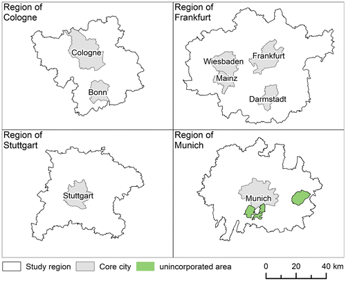
The study regions are four German city-regions: Cologne, Frankfurt, Munich and Stuttgart (Figure 1). These regions were roughly delineated on the basis of regional labour markets defined by the Federal Institute for Research on Building, Urban Affairs and Spatial Development.

Figure 1. Study regions and core cities.

Source: Author.

The analyses are conducted on the spatial level of grid cells with a side length of 1 km and located in accordance with the European grid INSPIRE (Infrastructure for Spatial Information in the European Community). Compared with municipality boundaries that are frequently used, grid cells allow for a more detailed picture and should help avoid false conclusions resulting from administrative boundary artefacts.

Data concerning employees are taken from the georeferenced Integrated Employment Biographies (georeferenced IEB), as of 30 June 2009, which are provided by the Research Data Centre of the Federal Employment Agency at the Institute for Employment Research (RDC). Originally, these are point data but these points must be aggregated into grid cells before the RDC may distribute them under German privacy laws (for aggregation details, see Scholz et al., 2012). Moreover, these aggregated data are subject to censoring also under German privacy laws. All grid cells with either less than three employees belonging to less than three firms (‘minimum case’) or one firm accounting for more than 50% or 75% of all employees (‘dominance case’) were censored (for details, see Bundesagentur für Arbeit, 2014). Thus, these grid cells had to be manually set to one, i.e., one employee, to avoid even more severe downward bias from completely excluding them from the analyses. However, the censored cells only contain 0.5–1.0% of all employees and 2.0–3.0% of the employees in service sectors in each study region. Employees in service sectors are those registered in sections J–N or S according to the Classification of Economic Activities, issue 2008 (WZ 2008). ³ Employees who are either not subject to social insurance or marginally employed were excluded because data on these groups were not available. For ease of reading, the term ‘employees’ will be used henceforth. It might be argued that these ‘subsets’ of all employees and the censoring spoil the validity of the analyses. However, the official data used herein are complete under German privacy laws. An imputation of employees not subject to social insurance, ⁴ such as self-employed persons, and rescaling them into grid cells would probably validate the comprehensive database but would not necessarily increase the quality of the analyses.

Earth observation images have shown the ongoing scattering of built-up areas for quite some time (e.g., Huang et al., 2007; Schneider & Woodcock, 2008). Recently developed methods allow for the derivation of built-up volumes (m³ per m² built-up area) from these images. Their computation was made possible for the first time on a fine spatial scale and over a large study region. Built-up volumes were calculated for the INSPIRE grid cells based on large-area three-dimensional building models for entire urban regions. These models were generated by fusing information from building footprints derived from topographic maps at a scale of 1:25 000 and building heights derived from these footprints with height measurements from stereoscopic satellite imagery (for details, see Wurm, d’Angelo, Reinartz, & Taubenböck, 2014). These models directly facilitate addressing the physical distribution of densities, which is one core element of morphological urban spatial structure (cf. the second section).

However, these data also contain built-up volumes for residential use only, which might bias the results. With the help of additional data from the Authoritative Topographic–Cartographic Information System (ATKIS Basis-DLM, shortly ATKIS), it was possible to eliminate these shares of ‘residential use only’ from the built-up volumes. Each ATKIS polygon is originally attributed with a type of use and when aggregating these polygons into the grid cell, the respective areas for each type of use are added together. Thus, the grid cell is assigned a value in m² for each type of use, out of which percentages per grid cell can be calculated. If ATKIS identifies x% of a grid cell’s built-up area to be designed for residential use, then the amount of built-up volumes in that grid cell is multiplied by to ‘remove’ the share of built-up volumes for residential use only. A point to ponder is that ATKIS and remote sensing data do not perfectly match, i.e., there are grid cells for which remote sensing identifies built-up volumes but ATKIS does not attribute any type of use. However, this mismatching accounts for at most 0.03% of the entire built-up area of a study region; thus, this limitation is considered negligible.

Empirical procedure and methods

The empirical procedure to detect spatial concurrence between employment and built-up volumes consists of two steps. First, spatial concurrence is analysed with the visual comparison of density maps and supported with Spearman’s rank correlation coefficients between employees, employees in service sectors, and built-up volumes, in addition to a coefficient on spatial autocorrelation, the global Moran’s I. Second, a statistical procedure based on exploratory spatial data analysis (ESDA) is applied to identify local spatial densifications (‘sub-centres’) taking into account spatial spillovers and statistical significance.

Density, as applied in the first step, means that the absolute number of employees in each spatial entity is divided by that entity’s area. Thus, it allows values for entities of different geographical size to be compared with one another. ⁵ Density is equal to absolute numbers here, as all grid cells are sized and shaped equally. However, there is an exception for those located at the regions’ fringes that are not fully covered: They are smaller than 1 km², but the qualitative and quantitative differences between density and absolute values are small in these particular cases. Spearman’s rank correlation coefficient is calculated using pairwise deletion and approximate p-values. Its significance is based on two-tailed tests without further adjustment. The global Moran’s I is calculated in accordance with Anselin (1995) by applying 9999 permutations and a pseudo-significance level of α = 0.001. Its formula is given in equation (1):

where I denotes the global Moran’s I for the region under consideration; and n is the number of spatial entities forming the study region. The spatial weights matrix consists of n × n row-standardized spatial weights ω _ij . Row standardization means that each ω _ij is divided by the row sum, which is equal to the number of non-zero row elements if a binary weight matrix is chosen. is the double sum of the weights, which is equal to n in case of row standardization. z _i and z _j are the respective observations measured in deviations from the mean, i.e., the mean x̄ of the study region’s observation value is subtracted from the spatial entity’s observation value x _i . The neighbourhood is defined as a second-order queen contiguity, which implies that entities sharing a common border or vertex with the one under consideration are assigned a ω _ij of 1. Additionally, these neighbouring entities’ direct neighbours are also assigned a ω _ij of 1. All others get no weight. Second-order queen contiguity was chosen because spatial spillovers are likely to have a larger influence than within a radius of approximately 1 km. ⁶

The global Moran’s I ranges between –1 and +1. These extremes imply perfect negative spatial autocorrelation, i.e., a ‘chequered’ pattern, and perfect clustering of similar values, respectively. A significantly positive value thus indicates that similar values are spatially grouped together, and a negative global Moran’s I indicates that rather different values are located in a common neighbourhood. However, a significantly positive global Moran’s I does not reveal information regarding whether high or low values are clustered. Values around zero imply that the spatial pattern is random.

Many of the methods used for the analysis of urban spatial structure thus far are mainly derivatives of monocentric city models. However, several scholars have shown that monocentricity is not the prevalent urban form, and some even argue that monocentric models might not even be relevant anymore (e.g., Arribas-Bel & Sanz-Gracia, 2014; Garcia-López & Muñiz, 2013). The application of an ESDA acknowledges this. It allows the identification of spatial patterns without an a priori assumption about their true nature. Independence from decisions regarding the locations of central business districts or threshold values is another advantage of ESDA, as it also reduces arbitrariness. Moreover, ESDA enables comparisons involving different spatial patterns in different regions because it only requires the choice of ‘framing parameters’, such as significance levels and/or neighbourhood definitions. In this study, ESDA is applied to both employees and built-up volumes to detect their respective spatial clustering and to thus draw conclusions regarding the study regions’ spatial configurations. Furthermore, theoretical contributions suggest that agglomeration economies such as knowledge spillovers are responsible for the spatial clustering of service sector employees, in particular (cf. Agarwal et al., 2012; Coffey & Shearmur, 2002; Muñiz & Garcia-López, 2010). Hence, a method that is able to detect spatial clusters seems reasonable. ⁷

Therefore, the measure of choice is the local Moran’s I as developed by Anselin (1995), one method of ESDA. This measure allows for the detection of clusters with high and low values, as well as spatial outliers, i.e., low values surrounded by high values and vice versa. This feature makes the local Moran’s I measure more attractive here than, for example, the application of the Getis and Ord’s G _i or G _i * statistic, which only identify spatial clusters but not spatial outliers. To describe extensively the urban spatial structure, it is necessary to identify both positive (clusters) and negative dependencies (outliers). Of course, applying ESDA cannot be the final step in analysing the morphological urban spatial structure. Instead, it is appropriate to analyse new data and to provide a descriptive assessment of their spatial distribution, which then should be further evaluated with respect to the forces causing it, for example. Because it is an exploratory method, the local Moran’s I reveals spatial patterns but does not offer a causal interpretation. It evaluates each spatial entity (in this case, each grid cell) in relation to its predefined neighbourhood, and its formula is presented in equation (2):

where I _i denotes the local Moran’s I for the spatial entity i. All other formula elements are the same as defined for equation (1). The neighbourhood definition again is according to second-order queen contiguity. Other scholars applying the local Moran’s I choose both similar (e.g., Arribas-Bel & Sanz-Gracia, 2014) and different neighbourhood definitions, such as the k-nearest or the average number of neighbours (e.g., Guillain & Le Gallo, 2010; Riguelle et al., 2007). This choice makes a difference if spatially irregularly shaped data are used but is of less relevance for grid cells because they are shaped regularly and sized equally. Differences in the number of neighbours for grid cells occur in the data used here in two cases: (1) when grid cells are located at the region’s edge and (2) when a non-empty grid cell is spatially adjacent to an empty cell because the latter are omitted from these calculations for technical reasons. Apart from that, the choice of the correct significance level in the presence of spatial autocorrelation is quite an issue. In the analysis below, it will be addressed as follows: First, local Moran’s I values are computed by applying 9999 permutations, as suggested by Anselin (1995) and later used by Arribas-Bel and Sanz-Gracia (2014). The resulting pseudo-significance level is set to α = 0.05 by convention. All results are saved and further processed to apply a false discovery rate, as suggested by Caldas de Castro and Singer (2006) based on the pseudo-p-value of α =0.05.

The local Moran’s I results include four types of spatial dependence: spatial clusters of high values surrounded by high values (high–high) or low values surrounded by low values (low–low). In this context, ‘high’ means above average (), and ‘low’ means below average (). Outliers are the opposite of the clustering of similar values, i.e., a high value surrounded by low values (high–low) or a low value is surrounded by high values (low–high). Interpreting the results requires some consideration as the local Moran’s I evaluates each grid cell’s variable against a local context defined by the weights matrix. Thus, areas without high values in absolute numbers but that have high values in relation to their neighbours can be considered high–high clusters, and vice versa. The same logic applies to spatial outliers: they are significantly different from their neighbours but not necessarily high or low in comparison with the entire study region.

The combination of these measurement approaches sheds new light on the urban spatial structure in Germany. Whereas the first step aims at inspecting the distribution of employees and built-up volumes – thus deriving hints about spatial clustering – the second step’s objective is to further support the results from the first step with the help of a statistically based measure that takes local contexts into account. The identified patterns will be presumptively explained with agglomeration economies, accessibility and topographic aspects. Establishing causal relationships based on the empirical analyses, however, is neither an objective nor a possibility.

Empirical findings

Location and correlation

Density maps (Figure 2) visualizing the location of employees and built-up volumes indicate obvious differences between the study regions’ urban spatial structure. Whereas the Stuttgart region shows a pattern that is quite dispersed in terms of employment and built-up volumes, the Munich, Cologne and Frankfurt regions are rather concentrated. The pattern in the Munich region is focused on the city of Munich, whereas the regions of Cologne and Frankfurt are characterized by the highest densities being located in the respective core cities. Therefore, from a visual assessment, it might be posited that Stuttgart is dispersed, that Frankfurt and Cologne are somewhat polycentric, and that Munich is monocentric. However, the polycentricity in both the Frankfurt and Cologne regions is also a matter of definition because both these regions consist of multiple core cities.

Figure 2. Standardized densities.

Source: Author’s own calculations based on the georeferenced IEB and data on built-up volumes.

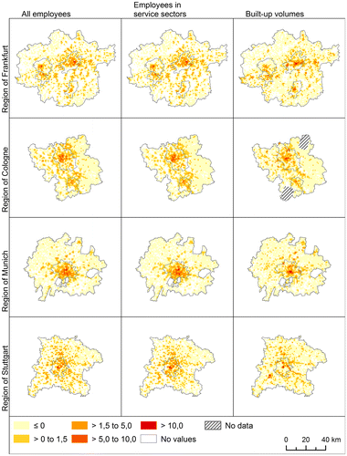
All data in Figure 2 were standardized into z-scores to make the variables and regions comparable. The colouring is identical for all maps: density increases as the colour changes from yellow to red. White areas do not contain the respective variable, and diagonally hatched areas indicate that remote sensing data were not available. Dark grey circled areas represent the core cities’ municipal boundaries.

A closer examination of Figure 2 reveals the spatial concurrence between employment and built-up volumes in the Frankfurt region. High densities are found in the core cities, whereas low densities are located in the region’s northern section, which is a low, mountainous area. The Cologne region shows similar patterns: the Bergisches Land area in the region’s eastern section contains only low numbers of employees and built-up volumes, whereas the highest densities are located in or near the core cities. The Cologne region and the Frankfurt and Stuttgart regions exhibit clustering tendencies within the core cities, which might hint at effective agglomeration economies. The Munich region clearly reveals a monocentric spatial configuration, although some outliers are discernible. The highest densities in the Stuttgart region are located along major roads and the River Neckar, which suggests a strong influence of accessibility issues and topography. Notably, the core city is not visually identifiable from the distribution of employees or built-up volumes. The urban spatial structure quite clearly shows a dispersed configuration with respect to employees and a quite obviously axial system with respect to built-up volumes, which is not particularly pronounced in any other region. To some extent, these consequences might ensue from topography: the region has been structured by several valley-like river canyons and ranges of hills surrounding the core city.

Furthermore, the impression of all density maps suggests that the level of spatial clustering is slightly higher for employees in service sectors than for all employees, whereas the concentration of built-up volumes is much higher than that of employees. The global Moran’s I values, which yield information regarding the degree of spatial association, provide quantitative evidence for this (Table 1). In contrast to the local Moran’s I, however, the global Moran’s I cannot distinguish the clustering of positive values from the clustering of negative values. Spatial association would be high in both cases because similar values are located together.

Table 1. global Moran’s I values.

	All employees	Employees in service sectors	Built-up volumes
Region of Cologne	0.4501	0.5074	0.4765
Region of Frankfurt	0.2981	0.3806	0.4149
Region of Munich	0.5828	0.6063	0.5999
Region of Stuttgart	0.2484	0.3282	0.2642

Note:

All values are significant at the 0.1% pseudo-significance level after 9999 permutations.

Source: Author’s calculations based on the georeferenced IEB and data on built-up volumes.

All values in Table 1 are positive and statistically significant implying significant spatial association in all study regions. The rather dispersed nature of the Stuttgart region is reflected in markedly lower global Moran’s I values than in the other regions. Conversely, the Munich region scores highest in all variables, which supports its position as ‘most monocentric’ region among the regions considered. However, the global Moran’s I does not reveal any information about the spatial concurrence of employees and built-up volumes. Thus, Spearman’s rank correlation coefficients are calculated to evaluate this issue (Table 2). All coefficients are also positive and statistically significant. The values for all employees and built-up volumes range between 0.65 in the Cologne and Frankfurt regions and 0.71 in the Stuttgart region. The Munich region scores 0.67. These values indicate medium correlations in all the regions. Thus, the proposition that employees are predominantly registered in grid cells containing built-up volumes and that their respective values are positively correlated (cf. the first section) is true. ⁸

Table 2. Spearman’s rank correlation coefficients.

	Built-up volumes
Region of Cologne
All employees	0.6475
Employees in service sectors	0.6337
Region of Frankfurt
All employees	0.6458
Employees in service sectors	0.6311
Region of Munich
All employees	0.6717
Employees in service sectors	0.6423
Region of Stuttgart
All employees	0.7061
Employees in service sectors	0.6825

Note:

All values are significant below the 1% significance level.

Source: Author’s calculations based on the georeferenced IEB and data on built-up volumes.

A closer look at Table 2 reveals that correlations among all employees and built-up volumes are higher than those between employees in service sectors and built-up volumes. These differences, however, are quite small within a region. One reason for this result, which contradicts the hypothesis expressed in the first section, might be found in the incomplete removal of built-up volumes for residential use. ATKIS helped remove shares that were for residential use only. However, there are many mixed-use areas in all the study regions, in particular, employees in service sectors are often located in mixed-use buildings. However, the built-up volumes for residential use in these buildings cannot be cleared by ATKIS. Thus, each employee is assigned more built-up volumes than she actually occupies, which yields lower correlations between the amount of built-up volumes and the number of service sector employees. All employees are also subject to this, but those who are not service sector employees are likely to be located in areas for industrial use only, which means that they are affected less and is further supported by small differences in the correlation coefficients (Table 2).

Exploratory analysis

Density maps (Figure 2), the global Moran’s I values (Table 1), and the correlation coefficients (Table 2) shed light on the spatial concentration and concurrence of high and low values of the variables under consideration but do not account for their local context. Thus, the next step is to detect statistically significant spatial clusters, which is essential for a full understanding of the urban spatial structure in a study region: density maps are likely to suffer from subjectivity because they only visualize values. Correlation coefficients shed light on coincidences of values, and spatial correlation coefficients yield information about the clustering of similar values. However, nothing is revealed about their spatial location and their actual and statistically significant pattern, and nothing can be said thus far about the actual existence, size and location of sub-centres.

Figure 3 visualizes the spatial clusters derived from the local Moran’s I values. Red-coloured areas indicate high–high clusters and blue-coloured areas indicate low–low clusters, whereas light red and light blue areas represent positive and negative outliers. White areas signify grid cells in which the values are either not registered or statistically insignificant. Grey areas indicate that the respective grid cell does not have a neighbour with a positive value (i.e., the neighbours are empty). Finally, remote sensing data were not available for diagonally hatched areas.

Figure 3. Cluster maps.

Source: Author’s own calculations based on the georeferenced IEB and data on built-up volumes.

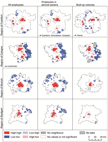
All study regions are characterized by the clustering of positive and negative values (bright red and blue areas in Figure 3), which is consistent with the significantly positive global Moran’s I values (cf. Table 1). There are also spatial outliers, but they do not occur excessively and thus do not substantially shape the urban spatial structure. The overall impression is of an urban spatial structure formed by significant high–high clusters mainly located in the core cities, which is particularly true for the Munich region ⁹ and also holds for the other regions. A closer look further reveals that there are more high–high clusters for all employees than for employees in service sectors. Therefore, the latter seem to be more concentrated, which might be an indication that they are either more exposed to positive – or suffer less from negative – agglomeration economies.

The Frankfurt region is characterized by a polycentric structure as the result of its four core cities. Furthermore, it is striking that there is a high–high building cluster in the region’s east (city of Hanau) that is not reflected in a high–high employee cluster. One explanation for this phenomenon might be that the number of employees is not markedly higher there than in neighbouring grid cells, thus yielding the local Moran’s I’s statistical insignificance. The density maps speak in favour of this explanation. The disappearance of a high–high cluster located between the Frankfurt region’s core cities when moving from all employees to those in service sectors is the result of industrial structure because that cluster captures an area in which the automotive sector is dominant. A ‘reverse’ situation applies to the municipalities of Eschborn, Schwalbach and Sulzbach, located directly north of the city of Frankfurt: although there is a small high–high cluster for all employees, it is much larger when employees in service sectors are considered, which is not surprising, because these municipalities host many offices and company headquarters. Furthermore, a comparison of the density maps (Figure 2) reveals that the high–high clusters coincide well with high-density areas. From an economic point of view, one might presume that agglomeration economies are effective both for all employees and those in service sectors, but the latter profit more.

When comparing the Frankfurt region with the Cologne region, the geographically larger amount of clustering in the latter is the most striking difference. Although there is an employment cluster north-east of Bonn if all employees are considered, this cluster disappears if only service sector employees are considered. To some extent, the same also applies to a high–high cluster in the city of Leverkusen, in which the chemical industry is predominantly located. These findings have the same background as in the Frankfurt region: after removing all the service sector employees, the remaining employees are too few to be significantly different from those in the neighbouring grid cells. The high–high clusters of built-up volumes match well with those for employees, which is further proof of the proposition that there is spatial concurrence between employees and built-up volumes.

An examination of the Munich region confirms that monocentricity characterizes the region. In contrast to the other study regions, this pattern does not change between all employees and employees in service sectors. However, the difference in the area covered by the high–high clusters is striking, for which the local Moran’s I does not provide a causal explanation, unfortunately. It might yet be assumed that positive agglomeration economies shape this distribution of employees. The lower clustering of built-up volumes – indicating a more equal distribution – might be the result of planning laws regulating the maximum amount of built-up volumes per square meter of ground floor.

The maps for the Stuttgart region speak in favour of a polycentric spatial structure. All variables exhibit significant positive clustering outside the core city. Although – or because – the automotive industry is dominant, the differences between the clustering of all employees and those in service sectors are comparatively small. However, the clustering patterns for built-up volumes are notably different. Although the spatial distribution of employees is polycentric, that of built-up volumes appears to be bipolar. It should be remembered that the area surrounding the clusters is not ‘empty’ but is rather not significant. Thus, this result suggests a rather dispersed urban spatial structure with two significant densifications of built-up volumes.

Synthesis and interpretation

The previous analyses show that the four study regions differ in their respective morphological urban spatial structures. Whereas the Stuttgart region is rather polycentric in terms of employees and seemingly bipolar in terms of built-up volumes, the Munich region clearly shows a monocentric pattern. The Frankfurt and Cologne regions are mainly characterized by their multiple core cities and economic structures in which the industrial sector is concentrated in certain areas of the region. Thus, these regions can be considered polycentric. However, their polycentricity is somewhat by definition because they consist of more than one core city (and thus more than one centre) rather than being characterized by actual sub-centre existence. A sub-centre is an area consisting of at least one grid cell being a statistically significant high–high cluster and either located outside the core city’s centre or in spatial distinction from the core city. From this perspective, all regions show polycentric patterns to different extents. From a theoretical point of view, one might thus argue that the Cologne and Frankfurt regions are inter-urban polycentric, whereas the Munich and Stuttgart regions tend to show intra-urban polycentricity (cf. Kloosterman & Musterd, 2001).

The combination of employees, employees in service sectors, and built-up volumes revealed insufficient detection of morphological urban spatial structure if not all these variables are considered. Although they show spatial concurrence, their distributions differ in details. The cluster maps (Figure 3) visualized this result and the two correlation coefficients (Tables 1 and 2) additionally support it. Thus, one variable suffices to gain a rough, but sometimes misleading, impression of a region’s urban spatial structure. However, important details resulting from the region’s industrial structure might remain unrevealed, such as in the Stuttgart region, which seems polycentric in terms of employees but is rather bipolar in terms of built-up volumes. We also observed some evidence of these differences in the Frankfurt region, where the three variables’ clusters differ markedly. In the quite monocentric region of Munich, additional information from two out of three variables seems negligible, which might lead to the conclusion that the more monocentric a region, the less important it is to have an encompassing data set. However, it is not a priori certain that monocentricity will occur (for all variables). In other words, because urban spatial structure in general and polycentricity in particular are complex concepts, their analysis requires a rich set of variables and indicators that extend beyond solely socioeconomic variables. This paper’s empirical results support this claim.

Conclusions and prospects

The analyses herein provided detailed insight into the urban spatial structure of four selected German city-regions. A high correlation of employees and built-up volumes was found, and their interplay certainly shapes the urban spatial structure. Although spatial concurrence between the variables considered applies for all regions under consideration, the respective outcomes differ. Whereas the Stuttgart region is polycentric for employees and – to a limited extent – for built-up volumes, the results for the Frankfurt and Cologne regions are not as unambiguous. Both regions show polycentric patterns but with obvious core city dominance. The Munich region is characterized by a strong core city and is thus monocentric, although there are single high–low outliers in the region’s periphery. Furthermore, it is remarkable that all the sub-centres in the regions are located in close proximity to a core city. These sub-centres differ markedly from American edge cities with respect both to their sizes – American edge cities are much larger spatially – and their location – American edge cities are mostly located at the edges of regions. An edgeless city pattern, sometimes considered ‘beyond polycentricity’ (Gordon & Richardson, 1996), does not yet exist in any study region study herein. Even in the most dispersed study region, Stuttgart, clusters of activity remain, and considering the urban spatial structure ‘flat’ would not appropriately reflect reality.

The empirical procedure employed herein and its results are unique in national research. Moreover, an integrated approach combining socioeconomic and remote sensing data has found its way into international research only fairly recently. The data on employees and built-up volumes are helpful in identifying clusters and outliers – which are similar in certain respects but different in others – jointly shaping the morphological urban spatial structure. However, the results gained here are just an approximation because the employment data utilized in this study suffer from both a rough classification of economic activity and censoring due to German privacy laws. Additionally, a more thorough removal of built-up volumes for residential use would further enhance the results’ quality and also open up routes for in-depth analyses of land use and land intensity in different industrial sectors.

Given the newly available data, it is now feasible to compare the actual location of employees and built-up volumes with planning goals, e.g., reaching the legally defined maximum inner city densities of built-up volumes. Moreover, combining employees and built-up volumes into one indicator (employees per m³ of built-up volumes) would enable the distinction between retail and office agglomerations, for example, shedding light on the quality of densifications and also likely on their economic resilience. However, a discussion of vacancies and of past, present and future industry structure, among other topics, would be required. All this work, unfortunately, requires much more comprehensive data than the data available for this study. To fully capture the urban spatial structure, it would also be revealing to consider population. The same applies to the use of panel rather than cross-sectional data. Development processes yielding the current urban spatial structure could not be analysed here but had to remain for further research. Finally, all the analyses conducted above are descriptive and exploratory but do not explain causalities. Thus, the next step would be to conduct regression analyses to reveal (mutual) causalities and to explicitly consider topics such as the influence of planning regulations and policies on the regions’ urban spatial structure.

Acknowledgements

The author would like to thank Michael Wurm from the German Remote Sensing Data Centre (DLR) for processing the remote sensing data and qualifying them with the ATKIS data, Theresa Scholz and Norbert Schanne from The Research Data Centre of the Federal Employment Agency at the Institute for Employment Research for the compilation of the grid data concerning employment and Stefan Siedentop for helpful comments.

Disclosure statement

No potential conflict of interest was reported by the author.

Additional information

Funding

The author’s current position at the Research Institute for Regional and Urban Development gGmbH (ILS), Dortmund, is funded by the German Research Foundation (DFG) [grant number SI 932/4-1].

Notes

1. The data on population data were, unfortunately, not available.

2. This list is far from exhaustive and contributions on topics such as sprawl, transportation and car dependence, or planning policies are not acknowledged because these aspects are beyond the scope of this paper.

3. These include information and communication (section J); financial and insurance activities (K); real estate activities (L); professional, scientific and technical activities (M); administrative and support service activities (N); and other service activities (S).

4. If all Germany is considered, employees subject to social insurance account for more than 75% of all people employed (Statistisches Bundesamt, 2008). Spatially disaggregated information on the distribution of the remaining 25% is not available.

5. For a discussion about ‘density’, see Fina, Krehl, Siedentop, Taubenböck, and Wurm (2014).

6. This is also implicitly assumed in other scholar’s work if they use a first-order queen contiguity on geographically larger entities.

7. Whether agglomeration economies are the true causes for the clusters that ESDA identifies is presumptive from a strictly quantitative point of view.

8. Spurious correlations are possible but this issue cannot be directly addressed with the data available. Nonetheless, there are reasons to believe that the correlations are robust and not driven by a ‘third party’.

9. Munich was more severely hit from censoring due to the ‘dominance case’ than the other regions, which must be considered when interpreting the results.

References

- Adolphson, M. (2009). Estimating a polycentric Urban structure. Case study: Urban changes in the Stockholm region 1991–2004. Journal of Urban Planning and Development , 135 , 19–30. doi:10.1061/(ASCE)0733-9488(2009)
- Agarwal, A. , Giuliano, G. , & Redfearn, C. L. (2012). Strangers in our midst: The usefulness of exploring polycentricity. The Annals of Regional Science , 48 , 433–450. doi:10.1007/s00168-012-0497-1
- Anas, A. , Arnott, R. J. , & Small, K. A. (1998). Urban spatial structure. Journal of Economic Literature , 36 , 1426–1464. Retrieved from http://www.jstor.org/stable/2564805
- Anas, A. , & Kim, I. (1996). General equilibrium models of polycentric Urban land use with endogenous congestion and job agglomeration. Journal of Urban Economics , 40 , 232–256. doi:10.1006/juec.1996.0031
- Anselin, L. (1995). Local Indicators of Spatial Association–LISA. Geographical Analysis , 27 , 93–115. doi:10.1111/j.1538-4632.1995.tb00338.x
- Arribas-Bel, D. , & Sanz-Gracia, F. (2014). The validity of the monocentric city model in a polycentric age: US metropolitan areas in 1990, 2000 and 2010. Urban Geography , 35 , 980–997. doi:10.1080/02723638.2014.940693
- Arribas-Bel, D. , & Schmidt, C. R. (2013). Self-organizing maps and the US urban spatial structure. Environment and Planning B: Planning and Design , 40 , 362–371. doi:10.1068/b37014
- Baumont, C. , Ertur, C. , & Le Gallo, J. (2004). Spatial analysis of employment and population density: The case of the agglomeration of Dijon 1999. Geographical Analysis , 36 , 146–176. doi:10.1111/j.1538-4632.2004.tb01130.x
- Bontje, M. , & Burdack, J. (2005). Edge cities, European-style: Examples from Paris and the Randstad. Cities , 22 , 317–330. doi:10.1016/j.cities.2005.01.007
- Bundesagentur für Arbeit. (2014). Statistische Geheimhaltung: Rechtliche Grundlagen und fachliche Regelungen der Statistik der Bundesagentur für Arbeit [Statistical confidentiality: Legal basis and technical regulations of the federal employment agency]. Nürnberg: Statistik der Bundesagentur für Arbeit.
- Caldas de Castro, M. , & Singer, B. H. (2006). Controlling the false discovery rate: A new application to account for multiple and dependent tests in local statistics of spatial association. Geographical Analysis , 38 , 180–208. doi:10.1111/j.0016-7363.2006.00682.x
- Carruthers, J. I. , Lewis, S. , Knaap, G.-J. , & Renner, R. N. (2010). Coming undone: A spatial hazard analysis of Urban form in American metropolitan areas. Papers in Regional Science , 89 , 65–88. doi:10.1111/j.1435-5957.2009.00242.x
- Coffey, W. J. , & Shearmur, R. G. (2001). Intrametropolitan employment distribution in Montreal, 1981–1996. Urban Geography , 22 , 106–129. doi:10.2747/0272-3638.22.2.106
- Coffey, W. J. , & Shearmur, R. G. (2002). Agglomeration and dispersion of high-order service employment in the Montreal metropolitan region, 1981-96. Urban Studies , 39 , 359–378. doi:10.1080/00420980220112739
- Craig, S. G. , & Ng, P. T. (2001). Using quantile smoothing splines to identify employment subcenters in a multicentric Urban area. Journal of Urban Economics , 49 , 100–120. doi:10.1006/juec.2000.2186
- Davoudi, S. (2003). EUROPEAN BRIEFING: Polycentricity in European spatial planning: From an analytical tool to a normative Agenda. European Planning Studies , 11 , 979–999. doi:10.1080/0965431032000146169
- Einig, K. , & Guth, D. (2005). Neue Beschäftigtenzentren in deutschen Stadtregionen: Lage, Spezialisierung, Erreichbarkeit [New employment centers in German city regions: Location, specialization, accessibility]. Raumforschung und Raumordnung , 63 , 444–458. doi:10.1007/BF03182973
- Farber, S. , & Li, X. (2013). Urban sprawl and social interaction potential: An empirical analysis of large metropolitan regions in the United States. Journal of Transport Geography , 31 , 267–277. doi:10.1016/j.jtrangeo.2013.03.002
- Fina, S. , Krehl, A. , Siedentop, S. , Taubenböck, H. , & Wurm, M. (2014). Dichter dran! Neue Möglichkeiten der Vernetzung von Geobasis-, Statistik- und Erdbeobachtungsdaten zur räumlichen Analyse und Visualisierung von Stadtstrukturen mit Dichteoberflächen und -profilen [Getting closer! New ways of integrating geodata, statistics and remote sensing to analyze and visualize Urban structures using density surfaces and -profiles]. Raumforschung und Raumordnung , 72 , 179–194. doi:10.1007/s13147-014-0279-6
- Garcia-López, M.-À. , & Muñiz, I. (2010). Employment decentralisation: Polycentricity or scatteration? The case of Barcelona Urban Studies , 47 , 3035–3056. doi:10.1177/0042098009360229
- Garcia-López, M.-À. , & Muñiz, I. (2013). Urban spatial structure, agglomeration economies, and economic growth in Barcelona: An intra-metropolitan perspective. Papers in Regional Science , 92 , 515–534. doi:10.1111/j.1435-5957.2011.00409.x
- Garreau, J. (1992). Edge city: Life on the new frontier (1st ed.). New York, NY : Anchor Books
- Giuliano, G. , & Small, K. A. (1991). Subcenters in the Los Angeles region. Regional Science and Urban Economics , 21 , 163–182. doi:10.1016/0166-0462(91)90032-I
- Glaeser, E. L. , & Gottlieb, J. D. (2006). Urban resurgence and the consumer city. Urban Studies , 43 , 1275–1299. doi:10.1080/00420980600775683
- Glaeser, E. L. , Kahn, M. E. , & Chu, C. (2001). Job Sprawl: Employment location in US. Metropolitan areas. Center on Urban & Metropolitan Policy Survey Series , 2001 , 1–8
- Gordon, P. , & Richardson, H. W. (1996). Beyond polycentricity: The dispersed metropolis, Los Angeles, 1970-1990. Journal of the American Planning Association , 62 , 289–295. doi:10.1080/01944369608975695
- Guillain, R. , & Le Gallo, J. (2010). Agglomeration and dispersion of economic activities in and around Paris: An exploratory spatial data analysis. Environment and Planning B: Planning and Design , 37 , 961–981. doi:10.1068/b35038
- Hall, P. , & Pain, K. (2006). The polycentric metropolis learning from mega-city regions in Europe . London: Earthscan.
- Hohenberg, P. M. (2004). The historical geography of European cities: An interpretive essay. In J. V. Henderson & J.-F. Thisse (Eds.), Handbook of regional and Urban economics. Cities and geography (1st ed.) (pp. 3021–3052). Amsterdam: Elsevier.
- Huang, J. , Lu, X. X. , & Sellers, J. M. (2007). A global comparative analysis of urban form: Applying spatial metrics and remote sensing. Landscape and Urban Planning , 82 , 184–197. doi:10.1016/j.landurbplan.2007.02.010
- Kloosterman, R. C. , & Musterd, S. (2001). The polycentric Urban region: Towards a research Agenda. Urban Studies , 38 , 623–633. doi:10.1080/00420980120035259
- Knapp, W. , & Volgmann, K. (2011). Neue ökonomische Kerne in nordrhein-westfälischen Stadtregionen: Postsuburbanisierung und Restrukturierung kernstädtischer Räume [New economic poles in the city regions of North Rhine-Westphalia: Postsuburbanisation and restructuring of the city]. Raumforschung und Raumordnung , 69 , 303–317. doi:10.1007/s13147-011-0112-4
- Kneebone, E. (2009). Job sprawl revisited: The changing geography of metropolitan employment (Metropolitan opportunity series). Washington, DC: Brookings. Retrieved from http://www.brookings.edu/~/media/research/files/reports/2009/4/06-job-sprawl-kneebone/20090406_jobsprawl_kneebone
- Lang, R. E. , & LeFurgy, J. (2003). Edgeless cities: Examining the noncentered metropolis. Housing Policy Debate , 14 , 427–460. doi:10.1080/10511482.2003.9521482
- Larsson, J. P. (2014). The neighborhood or the region? Reassessing the density–wage relationship using geocoded data. The Annals of Regional Science , 52 , 367–384. doi:10.1007/s00168-014-0590-8
- McDonald, J. F. (1987). The identification of urban employment subcenters. Journal of Urban Economics , 21 , 242–258. doi:10.1016/0094-1190(87)90017-9
- McMillen, D. P. (2001). Nonparametric employment subcenter identification. Journal of Urban Economics , 50 , 448–473. doi:10.1006/juec.2001.2228
- McMillen, D. P. , & McDonald, J. F. (1997). A nonparametric analysis of employment density in a polycentric city. Journal of Regional Science , 37 , 591–612. doi:10.1111/0022-4146.00071
- McMillen, D. P. , & McDonald, J. F. (1998). Suburban subcenters and employment density in metropolitan Chicago. Journal of Urban Economics , 43 , 157–180. doi:10.1006/juec.1997.2038
- McMillen, D. P. , & Smith, S. C. (2003). The number of subcenters in large Urban areas. Journal of Urban Economics , 53 , 321–338. doi:10.1016/S0094-1190(03)00026-3
- Meijers, E. J. , & Burger, M. J. (2010). Spatial structure and productivity in US metropolitan areas. Environment and Planning A , 42 , 1383–1402. doi:10.1068/a42151
- Muñiz, I. , & Garcia-López, M.-À. (2010). The polycentric knowledge economy in Barcelona. Urban Geography , 31 , 774–799. doi:10.2747/0272-3638.31.6.774
- Parr, J. B. (2014). The regional economy, spatial structure and regional Urban systems. Regional Studies , 48 , 1926–1938. doi:10.1080/00343404.2013.799759
- Pfister, N. , Freestone, R. , & Murphy, P. (2000). Polycentricity or dispersion? Changes in center employment in metropolitan Sydney, 1981 to 1996. Urban Geography , 21 , 428–442. doi:10.2747/0272-3638.21.5.428
- Redfearn, C. L. (2007). The topography of metropolitan employment: Identifying centers of employment in a polycentric urban area. Journal of Urban Economics , 61 , 519–541. doi:10.1016/j.jue.2006.08.009
- Riguelle, F. , Thomas, I. , & Verhetsel, A. (2007). Measuring Urban polycentrism: A European case study and its implications. Journal of Economic Geography , 7 , 193–215. doi:10.1093/jeg/lbl025
- Romero, V. , Solís, E. , & de Ureña, J. M. (2014). Beyond the metropolis: New employment centers and historic administrative cities in the Madrid global city region. Urban Geography , 35 , 889–915. doi:10.1080/02723638.2014.939538
- Schneider, A. , & Woodcock, C. E. (2008). Compact, dispersed, fragmented, extensive? A comparison of Urban growth in twenty-five global cities using remotely sensed data, pattern metrics and census information. Urban Studies , 45 , 659–692. doi:10.1177/0042098007087340
- Scholz, T. , Rauscher, C. , Reiher, J. , & Bachteler, T. (2012). Geocoding of German administrative data: The case of the institute for employment research ( No. 09/2012 EN).
- Scott, A. J. (2008). Resurgent metropolis: Economy, society and Urbanization in an interconnected world. International Journal of Urban and Regional Research , 32 , 548–564. doi:10.1111/j.1468-2427.2008.00795.x
- Siedentop, S. (2008). Die Rückkehr der Städte? Zur Plausibilität der Reurbanisierungshypothese [City’s comeback? On the plausibility of the reurbanization hypothesis]. Informationen zur Raumentwicklung , 2008 , 193–210.
- Siedentop, S. , Kausch, S. , Einig, K. , & Gössel, J. (2003). Siedlungsstrukturelle Veränderungen im Umland von Agglomerationsräumen [Spatial structural changes in the hinterland of conurbations] (Forschungen No. 114). Bonn: Selbstverlag des Bundesamtes für Bauwesen und Raumordnung.
- Smith, D. A. (2011). Polycentricity and sustainable Urban form. An Intra-Urban study of accessibility, employment and travel sustainability for the strategic planning of the London region ( Dissertation). University College London, London, UK.
- Statistisches Bundesamt. (2008). Bevölkerung und Erwerbstätigkeit: Struktur der sozialversicherungspflichtig Beschäftigten [Population and employment: the structure of employees subject to social insurance] ( Fachserie 1 Reihe 4.2.1). Wiesbaden: Statistisches Bundesamt.
- Wurm, M. , d’Angelo, P. , Reinartz, P. , & Taubenböck, H. (2014). Investigating the applicability of Cartosat-1 DEMs and topographic maps to localize large-area Urban mass concentration. IEEE Journal of Selected Topics in Applied Earth Observations and Remote Sensing , 7 , 4138–4152. doi:10.1109/jstars.2014.2346655
- Yang, J. , French, S. , Holt, J. , & Zhang, X. (2012). Measuring the structure of U.S. Metropolitan areas, 1970–2000. Journal of the American Planning Association , 78 , 197–209. doi:10.1080/01944363.2012.677382