When rural boroughs turn into inner peripheries: a link between their socioeconomic characteristics and distance to large cities

ABSTRACT

Inhabitants of rural areas are subject to several pressures such as depopulation, income gap and infrastructure scarcities compared with urban areas. An analysis of rural boroughs in Poland is carried at the LAU-2 (NUTS-5) level, based on sustainable development framework indicators with the use of logit models, in order to verify the existence of heterogeneities among rural boroughs caused by metropolitan area spillovers. The research shows that the deconcentration hypothesis holds only for rural boroughs within 40 km of large towns. The remaining rural boroughs have a profile of inner peripheries – they are subject to adverse demographic and development pressures, with limited infrastructure stock and public services availability. These remarkable differences between rural boroughs imply the need for a reconsideration of the criteria for regional Cohesion Policies. Namely, more location-dependent regional policy instruments should be designed instead of the currently prevailing approach based on NUTS-2 criteria.

KEYWORDS:

• convergence process
• inner peripheries
• regional disparities
• rural boroughs

JEL CLASSIFICATIONS:

• O18
• R11
• R50

INTRODUCTION

Designing effective policies aimed at reducing regional disparities is among the key challenges for decision-makers. Important determinants for such policies are the interactions between urban and rural areas on economic, social and demographic fields, as well as associated urbanization trends. In Europe, 27% of the population lived in rural areas in 2015, according to a United Nation’s (UN) (2015) report. Among the European Union (EU) countries, the lowest ratio was in Belgium (2%), Malta (5%), Iceland (6%) and the Netherlands (10%). The highest was in Romania and Slovakia (46%). In Poland, it amounted to 40% (pp. 38, 50, 233). Generally, the inhabitants of rural areas are subject to several pressures, such as depopulation, income gap and infrastructure scarcities. Particularly in developing countries, there is a clear development gap between rural and urban areas (to the detriment of rural areas), reflected by measures of living standards and the availability of social infrastructure, for example, in the fields of education and healthcare (Organisation for Economic Co-operation and Development (OECD), 2016, pp. 20–21).

Regardless of the level of development of a given country, a general regularity is noticeable, that the increase in urbanization is associated with a higher level of economic development of the country, and at the same time with a growing gap between the affluence of urban and rural areas. Although the direction of this relationship (its causality) is not always clear and the paths of income growth vary between countries, urban areas are clear centres of economic activity characterized by higher incomes (UN, 2015, p. 34).

However, it should be noted that the key here may not be the rural character of a given entity but its geographical location. Wherein, the distance parameter does not mean a linear increase of the shortcomings of a given rural borough (RB). According to the deconcentration hypothesis, which states that the population moves to rural areas for lifestyle and quality-of-life reasons, while retaining urban employment through rural-to-urban commuting, up to a specific distance the proximity of an urban area exerts a positive influence on RBs. This phenomenon is possible due to the diminishing cost of distance and is additionally propelled by the increasing negative externalities within urban areas. The theory dates back to such quantitative studies as Wardwell (1980) and Long (1981). A broad review of studies on agglomeration economies, and interdependencies between urban and rural areas as well the significance of peripheral location, is presented by Gruber and Soci (2010). Several pieces of research based on the New Economic Geography or the core–periphery set-up in general support the hypothesis of advantages of agglomeration proximity on rural areas.

Such phenomena are confirmed by research on the performance of regions with a different profile (below the NUTS-3 level). Dijkstra, Garcilazo, and McCann (2015) showed that, in the EU specifically, the rural remote regions and the urban regions were more vulnerable to the crisis that started in 2007–08. Research results do not support the models of regional convergence of these entities from the perspective of gross domestic product (GDP), productivity and employment indicators. The city-led growth pattern, which prevailed before the crisis, was also inverted as a result of the crisis. The relative beneficiaries during that period were the intermediate regions and the rural regions adjacent to municipal areas. In another study, Townsend and Champion (2014) reported that the costs of recession in 2008 in the UK, evaluated by employment levels, were to a greater extent borne by peripheral local governments (LGs), both urban and rural. The analysis of rural areas in Poland at the LAU-2 level by Kluza and Rafał (2018) confirmed the existence of two distinctive profiles of RBs: systematically depopulated and financially stressed peripheral boroughs and RBs adjacent to large municipalities, which undertook skilful free rider strategies. The latter limited their own provision of public goods such as healthcare, and education, on the one hand, and, on the other, attracted residents and businesses at the cost of the neighbouring municipalities.

Several pieces of research present the relative importance of geography and institutions for economic development at a subnational level (see a study and literature review in Mitton, 2016). They showed that geographical variables play a more important role than institutional framework in explaining GDP per capita levels. Moreover, geographical location exerts an influence on the entrepreneurial and innovation characteristics of a given area. Studies conducted by Artz, Kim, and Orazem (2016) show direct positive agglomeration effects on the entry of new firms to the market. Firms are more likely to locate in markets with an existing cluster of firms in the same industry, with higher concentrations of upstream suppliers or downstream customers, and on the market with a bigger local pool of college-educated workers. Such benefits appear in both urban areas as well as adjacent rural areas, which are within a commuting distance. They directly translate into greater economic prosperity of these regions.

The spatial concentration, especially with respect to production, influences the region’s ability to generate innovations through knowledge spillovers and as a result it promotes faster economic growth (for a review, see Feldman, 1999). As the research by Crescenzi (2005) shows, a location of regions had a direct impact on their innovation capabilities. Peripheral regions required much larger investments in human capital in order to maintain equal productivity as core areas. McCann and Folta (2011) and Hervas-Oliver, Sempere-Ripoll, Rojas Alvarado, and Estelles-Miguel (2018) show that firms’ innovative performance or general performance is attributable mainly to positive externalities generated by localization in agglomerations or business clusters. Marek, Titze, Fuhrmeister, and Blum (2017) obtained statistically significant models for German NUTS-3 regions, which show a decreasing relationship between geographical distance and research and development (R&D) collaboration. The threshold value for the geographical distance amounted to 50 km. In addition, the effect of technological distance turned significantly negative when the geographical distance was > 50 km.

Partridge, Ali, and Olfert (2010) show the interdependencies between urban and RBs in Canada and how the agglomeration economies can spill over to surrounding areas. Their findings strongly support the deconcentration hypothesis, which reflects the positive effects exerted by agglomerations on RB due to their proximity to large cities. For rural areas within the commuting distance, urban employment is a key source of population retention and growth, with distance representing a primary restraint. In addition, the job growth is negatively correlated with rural areas remoteness. For Canada, the commuting distance from rural areas, which supports the deconcentration hypothesis, amounts to up to 120 km (but with a mean distance of 61 km). Similarly, McArthur, Thorsen, and Ubøe (2010) model the spatial unemployment disparities in Norway. The study shows that they sharply grow when the distance between two regions > 80 km.

Renkow and Hoover (2000) showed that for rural areas in North Carolina, United States, the 35 miles distance (60 km) is the boundary of a different character of the migration behaviour of residents. Up to 35 miles, these areas constitute the direct labour backing for urban areas thanks to work commuting. A subsequent study by Renkow (2003) for rural and urban areas in North Carolina showed that half of new metro jobs and one-third of new rural jobs were filled by (non-residents) in-commuters. Lewin, Weber, and Holland (2013) show that over the last decades the commuting linkages grew stronger in the core–periphery set-up. At the same time, the sales and purchases of goods and related business activities have gradually declined, leading to mainly labour and demographic interactions between the core and periphery. Thus, the commuting effects on employment gained in importance. Ganning, Baylis, and Lee (2013) extended the research of metropolitan spillovers on non-metropolitan communities in the United States by testing not only the nearest city impact but also the inverse-distance model and relative commuting flow to multiple cities. The inverse-distance model of multiple cities turned out to be most solid, yielding the result that spread effects have an impact on population trends in non-metropolitan areas up to 60–90 miles depending on the metropolitan city size. The models also showed that income change is positively correlated with non-metropolitan growth, while initial year income is negatively related to growth (i.e., growth in urban income results in spread effects).

Confirmation of the deconcentration hypothesis has several implications – in particular, it means that all rural areas cannot be treated homogeneously in regional policies as they have deeply distinctive socioeconomic profiles, varying with their location. Thus, the ‘one size fits all’ approach in the EU allocation policies, which is derived from the fact that the eligibility and financial allocations for the regional policies are largely determined on the NUTS-2 level, may lead to stimulation of stronger regions at the expense of weaker regions. Problems of this nature are confirmed by several studies on the effectiveness of the Cohesion Policy, whose main goal is ‘reducing disparities between the various regions and the backwardness of the least-favoured regions’ as defined in the 1986 Single European Act.

The effectiveness of Cohesion Policy activities is widely studied in the research literature and the results deliver several controversies about the positive, neutral or even negative impact of the EU policies on the regional convergence process. Their recent review is presented in Fratesi and Wishlade (2017). The research findings range from policies’ immediate positive impact on reducing disparities between core and peripheral areas in Europe, through positive impact over time, to neutrality of the EU regional policies or even negative impact on growth (the latter are presented in, for example, Bouayad-Agha, Turpin, and Védrine, 2013; and Puigcerver-Peñalver, 2007).

Boldrin and Canova (2001), in a broad statistical analysis of the regions in EU-15 countries from the 1980s to 1996, showed that there is no evidence of either decreasing or growing disparities between regions. The EU regional policies are mainly redistribution policies driven by political, not economic, factors. An assessment of EU Cohesion Policy in Italy conducted by Aiello and Pupo (2012) showed that, despite the higher impact of Structural Funds on underdeveloped regions, they did not manage to reduce the long-lasting productivity differences between the south and centre-north of the country.

The majority of research shows a positive impact of the EU regional policies, emerging over different time horizons. A recent study by Jakubowski (2018) showed both the β- and σ-convergence for the EU regions in 2004–14. A broad review of the quantitative results of 17 research papers is presented by Dall’erba & Fang (2017). They also provide an explanation why the results of different studies are so differentiated. Heterogeneity comes from, among others, the period examined, the control of endogeneity and the presence of several regressors other than Structural Funds. They point out that ‘more attention could be given to locally weighted estimates of the funds …  to provide coefficient estimates for every single region, as opposed to the average impact for the entire sample’ (p. 831).

Several pieces of evidence of regional convergence do not equal a confirmation of regional policy effectiveness. Gagliardi and Percoco (2017) carried out research on the heterogeneous local responses to the 2000–06 European Cohesion Policy. The analysis was undertaken at the NUTS-3 level, which allowed then to show that specific areas that should not be eligible for the policy support as characterized by the 75% of the EU average GDP per capita threshold received the funds because the eligibility criterion was applied at a broader geographical scale (based on NUTS-2 typology). Such an ‘inadequacy’ had vital implications for some regions. Specifically, it was beneficial for rural areas close to city centres. Owing to a combination of such factors as support of the EU funds, geographical location and availability of space to accommodate the flow of people and new activities, they outperformed not only more dispersed rural areas but also urbanized and suburbanized areas. Potential inefficiencies and disorders resulting from the misdirected Cohesion Policy can be substantial. In the 2014–20 Financial Perspective, the European Commission allocated €371.4 billion (after amendments) for such policies, which constitute 34% of the total EU budget for the 2014–20 period. The eligibility and financial allocations for the regional policies are largely determined at the NUTS-2 level.

The topics of urban–rural convergence/divergence and the choice of relevant policy instruments are complex and deliver mixed analysis results in the research literature. In this paper, we intend to deepen the knowledge on factors that lay behind the performance of various rural regions, in such fields as disparities in income, infrastructure stock, employment and demographics, taking into account their location from major urban centres, namely capital cities of Polish provinces. Acquiring information on significant differences in the profiles of rural areas is the key to designing and implementing well-tailored policies supporting regional convergence. As shown by Dijkstra et al. (2015) and Gagliardi and Percoco (2017), more detailed geographical analyses unveil several significant heterogeneities in the profiles of LGs which affect the outcomes of the rural Cohesion Policies.

In this paper we carried out the analyses for the LAU-2 Eurostat territorial typology (corresponding to the former NUTS-5 level). There are 2808 LG entities as of 2016 in Poland. They form a three-tier system, which consists of boroughs, counties and provinces. The largest towns (66 entities at the end of 2016, including provincial capitals – PCs) perform both the functions of boroughs and counties, and they form a separate category called ‘towns with county rights’. Boroughs are split into three categories: municipal boroughs, municipal-RBs and RBs. The RBs are defined as areas composed only of villages and minor settlements – they cannot contain urban areas with municipal rights. RBs are relatively small entities and sparsely populated compared with other LG categories, especially PCs (Table 1).

Table 1. Area and population of selected local government categories in Poland; data for 2016.

	Rural boroughs	Municipal-rural boroughs	Municipal boroughs	Towns with county rights	of which:
					Provincial capitals	Other towns with county rights
Entities	1559	616	237	66	18^a	48
Total area (km^2)	194,868	103,696	6717	7398	3759	3639
Average area (km^2)	125	168	28	112	209	76
Median area (km^2)	110	147	22	85	171	71
Total population (persons)	10,942,514	8,902,730	5,972,023	12,619,972	7,650,846	4,969,126
Average population (persons)	7019	14,452	25,198	191,212	425,047	103,523
Median population (persons)	5915	11,724	20,572	112,483	319,289	90,909

Note: ^aThere are 16 provinces in Poland; however, in two cases, the provincial capitals are co-located in two towns.

Source: ‘Area and Population in the Territorial Profile in 2016’, Central Statistical Office of Poland (GUS).

In this research, we focus solely on RBs and their interactions with urban areas. RBs are the most numerous LG category, which reflect the rural areas the best. We intend to contribute to the existing literature by showing the link between socioeconomic characteristics of these rural areas and their geographical location. The aim of the research is to verify up to which distance the positive spillovers between agglomeration and RBs take place, being consistent with the deconcentration hypothesis, and, accordingly, when negative socioeconomic effects emerge.

The paper is organized as follows. Next, we describe the modelling approach used in this research. The RBs are described by several indicators reflecting the general sustainable development framework (social, demographic, economic, environmental, etc.). We then design several models based on the distance to a PC. We validate these results with models based on the distance to the nearest town with county rights as well as a simplified multiple-centre concept, inspired by the research of Ganning et al. (2013). We use logit models, which are suitable tools for estimating binary dependent variables. In this case, they describe what the probabilities are that certain socioeconomic indicators are interrelated with an RB located at a specific distance from the large urban area. The models enable one to identify the specific distances for which particular socioeconomic differences noticeably materialize in RBs.

MODELLING APPROACH AND DATA

Econometric modelling in this research is conducted with the use of the logistic regression (logit) model. Logit models are dedicated and widely used for modelling the discrete dependent variables (e.g. Greene, 2000, ch. 19; Verbeek, 2002, ch. 7). The sources of the data used in the third section are indicated in Table 2. In our case, we model a binary variable, i.e.:(1) $Y_i=\left\{\begin{array}{cc}1,& \mathrm{i}\mathrm{f}\mathrm{a}\mathrm{r}\mathrm{u}\mathrm{r}\mathrm{a}\mathrm{l}\mathrm{b}\mathrm{o}\mathrm{r}\mathrm{o}\mathrm{u}\mathrm{g}\mathrm{h}\mathrm{s}\mathrm{a}\mathrm{t}\mathrm{i}\mathrm{s}\mathrm{f}\mathrm{i}\mathrm{e}\mathrm{s}\mathrm{a}\mathrm{s}\mathrm{p}\mathrm{e}\mathrm{c}\mathrm{i}\mathrm{f}\mathrm{i}\mathrm{c}\mathrm{c}\mathrm{o}\mathrm{n}\mathrm{d}\mathrm{i}\mathrm{t}\mathrm{i}\mathrm{o}\mathrm{n}\left(\mathrm{i}.\mathrm{e}.\mathrm{d}\mathrm{i}\mathrm{s}\mathrm{t}\mathrm{a}\mathrm{n}\mathrm{c}\mathrm{e}\right)\\ 0,& \mathrm{o}\mathrm{t}\mathrm{h}\mathrm{e}\mathrm{r}\mathrm{w}\mathrm{i}\mathrm{s}\mathrm{e}\end{array}\right.$(1) The conditions analysed for the RBs are presented in the third section. The logistic function has the following form:(2) $p_i=P\left(Y_i=1|X_i;a\right)=\frac{1}{1+e^{-Z_i}}=\frac{e^{Z_i}}{1+e^{Z_i}}$(2) where Z is a linear function such that $Z_i=a_0+a_1{X}_{1i}+a_2{X}_{2i}+\dots +a_k{X}_{ki}+{\epsilon }_i$; i is the number of observations; X_k is the independent variables (in this case the socioeconomic characteristics of RBs); $k=1,2,\dots ,n$ is the number of variables; a_k is the coefficients; and a₀ is a constant.

Table 2. Variables used in final model specifications.

Variable	Description
Demographics
pop_change	Population change for the 2012–16 period
pop_pre_prod	Share of the population at pre-working age in the total population (2016)
pop_post-prod	Share of the population at post-working age in the total population (2016)
pupils_in_popul	Pupils in primary schools per 1000 inhabitants (2015)
Business and labour
firms_pc	Business registered in REGON per 1000 inhabitants (2016)
salary	Monthly gross salary – compared with national average (Poland = 100); data for the counties (2015)
Social and infrastructure
apartments_pc	Dwellings completed per 1000 inhabitants (2016)
HealthBasic	Health out-patient entities per 10,000 population (2016)
kind_garten	Children of age 3–6 years covered by preschool education (2014)
water	Persons using water supply system as a % of the total population (2015)
Local government (LG) financials
Rev_pc	LG operating revenue per capita (2016)
Environmental
forest	Share of forest areas in the total area of rural borough (2016)
tourist^a	Number of bed places in tourist facilities (2016): 0 = ≤ 10 beds; 0.2 for (11–100) beds; 1.0 for (101–500) beds; 2.0 for (501–5000) beds; 3.0 for > 5000 beds

Note: ^aThe ‘tourist’ variable was standardized into five brackets owing to its very high coefficient of variation (503%).

Sources: All statistics are from Central Statistical Office of Poland (GUS), except for the indictors reflecting LG operating revenue, which are taken from the Ministry of Finance of Poland.

There are two primary ways of interpreting the model results. The sign of a_k coefficient reflects an impact’s direction of the independent variable on the probability of $Y=1$. The impact magnitude of a given variable change on obtaining the probability of 1 by the dependent variable is measured by a marginal effect, defined as:(3) $\frac{\mathrm{\partial }{p}_i}{\mathrm{\partial }{x}_{ki}}=\frac{\mathrm{\partial }{\displaystyle \frac{e^{Z_i}}{1+e^{Z_i}}}}{\mathrm{\partial }{x}_{ki}}=a_k{p}_i\left(1-p_i\right).$(3) It is important to notice that marginal effects for different variables are directly comparable only in the case of variables which are described in similar nominal terms. Denominating a variable will affect its a_k coefficient, which in turn will affect the magnitude of a marginal effect.

In this research, the primary analysis is devoted to the relationship between the socioeconomic properties of RBs and their distance to the nearest PC (not necessarily to the one which is its administrative capital). The distance reflects the distance between the centre of the respective PC and the centre of the RB (location of its administrative authorities). Typically, inhabitants of such RBs are spread in the area of ±10–15 km around the RB centre. In the designed models, the analysed distance is reflected by the Euclidean distance between the two centres (GEO coordinates), which is relatively the simplest but also the most objective measure. Alternative measures are, for example, the travel time between two points (e.g., Ejermo and Karlsson, 2006). These measures are more precise for evaluating population characteristics; however, they depend on several other factors (most of all traffic intensity).

In order to capture the socioeconomic disparities of RB, we refer in this research to the general framework of development sustainability (UN, 1987, p. 16). There are various aspects of sustainability and its measurement. They cover such areas as, among others, poverty, economic development, health, education, demographics, natural hazards, consumption and production patterns, etc. They also encompass the infrastructure and quality-of-living indicators, for example, the proportion of population using an improved sanitation facility is one of the six core indicators within the theme of poverty (UN, 2007). Although these indicators were mainly designed for the country level, several might be easily adjusted to the regional policies context. Specific indicators for analysing rural development are presented, for example, in Adamowicz and Smarzewska (2009), Borys (2008), Firmino Costa da Silva, Elhorst, and Silveira Neto (2017), and Kluza and Rafał (2018). The indicators used in this research are shown in Table 2.

In the first part of our research, we employ three approaches using the logit models to capture the relationship between the distance variable (Y) and socioeconomic properties of RBs (Figure 1). Approach 1 is based on the comparison of characteristics of eight models (eight distinctive logistic regressions), where Y = 1 for a different distance parameters d between a PC and an administrative centre of a given RB. The distance parameter d is defined as d ≥ (10 km·i + 10 km), where i is the model number from 1 to 8. That means that for the model 1 in this approach, Y = 1 is satisfied for all RBs located no closer than 20 km from the PC (it covers 93% of RBs); for model 2, Y = 1 is satisfied for all RBs no closer than 30 km (it covers 85% of RBs), and so on up to model 8, where Y = 1 is satisfied for all RBs no closer than 90 km (it covers the furthest 8% of RBs). All the RBs in the subsequent models are subsets of RBs in the models with lower i parameter.

Figure 1. Three approaches used in modelling: illustration of basic differences. Source: Author’s own elaboration.

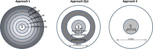
Approach 2(a) consists of a comparison of five models (five distinctive logistic regressions), where Y = 1 for different distance zones between a PC and an administrative centre of a given RB. The distance parameter d is defined as d ∈ [20 km·i – 20 km; 20 km·i), where i is the model number from 1 to 4 and d ≥ (20 km·i – 20 km) for i = 5. As a result, five disjunctive sets of RBs, grouped in 20 km distance layers, are analysed. In addition, to check whether there is no subjective mistake in selecting 20 km as the initial distance for the layers, a comparable modelling – Approach 2(b) – is conducted for d ∈ [20 km·i – 10 km; 20 km·i + 10 km), where i is the model number from 1 to 4 and d ≥ (20 km·i – 10 km) for i = 5.

Finally, Approach 3 is based on the results of the previous two approaches. Their outcomes allow to split the RBs into two disjunctive sets only, which disclose different socioeconomic characteristics of RBs depending on the parameter d. The three approaches described delivered models which were statistically significant and with high accuracy ratios. In addition, the obtained results are verified against two other modelling approaches, based on Ganning et al. (2013). First, they are compared with the model where PCs are replaced with all the towns with county rights (66 entities including PCs), as they also may be a source of agglomeration spillovers for RBs. Second, they are compared with the model in which RBs were selected based on the condition that the distance between their nearest PC and their nearest town with county rights was < 30 km (1001 of 1559 RBs satisfy this condition). This model is a proxy for multiple city analysis. The selected results of the described analyses are presented in the third section and in Tables A1–A3.

DISCUSSION

For final model specification, 11 variables were selected – such that meaningfully described the characteristics of peripheral RBs (Table 2). The selection was carried out based on statistical significance analysis of individual variables and Akaike’s information criterion. These variables corresponded, in particular, to demographic characteristics such as population growth, percentage of pupils in primary schools, share of the population at pre- and post-working age in the total population, variables reflecting economic conditions such as salary, number of registered companies per inhabitant, and variables reflecting quality of social and communal infrastructure, such as children of age 3–6 years covered by preschool education, persons using the water supply system as a percentage of the total population, health out-patient entities per 10,000 population, LG financials measured by total revenues per capita and share of forest areas in the total area of the RB.

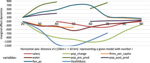
The analysis of the results of the estimation for the models from Approach 1 reveals that the changing profile of RB is linked to the degree of their peripheral location. The strongest marginal effects for variables, that is, the impact of a given variable on the probability that a given RB is a depressed peripheral RB, occur in the case of units located a minimum of 40 km from a PC (Table 3).

Table 3. Summary of the results for Approach 1: marginal effects of statistically significant variables for all estimated models.

Distance from a provincial capital (km)	≥20	≥ 30	≥ 40	≥ 50	≥ 60	≥ 70	≥ 80	≥ 90
salary			−0.003	−0.006	−0.010	−0.010	−0.005	−0.003
pop_change	−0.459	−2.907	−4.120	−4.548	−5.156	−4.606	−2.684	−1.161
pupils_in_popul		−0.003	−0.005	−0.006	−0.007	−0.008	−0.004	−0.002
kind_garten	−0.001		−0.001^a	−0.003		−0.001	−0.002	−0.002
firms_per_capita	−0.001	−0.002	−0.002	−0.002		0.002	0.001	0.001
forest			0.003	0.003	0.002	0.001	0.001	0.000^a
water	−0.001	−0.002	−0.002	−0.003	−0.002	−0.001	−0.001	0.000^a
pop_pre_prod	0.004	0.027	0.035		0.021^a	0.033
pop_post_prod	0.004	0.009	0.012^a		−0.015	−0.010^a	−0.009	−0.004^a
Rev_pc	0.022	0.075	0.105	0.156	0.152	0.033	0.021	0.011
HealthBasic	−0.002	−0.010	−0.025	−0.026	−0.021	−0.014
% of all RBs	93%	85%	73%	58%	42%	27%	15%	8%

Note: ^aVariables with a significance between 10% and 20%; skipped values denote insignificant variables for a given model.

Source: Author’s own calculations.

Limiting the sample to RBs with a distance of no less than 50–60 km increases the strength of some of the marginal effects, whereas it happens at the expense of losing the statistical significance of selected variables. This indicates the potential existence of a border distance that causes rural communes to suffer from their peripheral location. For d ≥ 70 km, marginal effects visibly shrink. The fitness of the model is weakening if we consider only RBs located > 90 km from a PC. To some extent, this may be the effect of the small size of this group – < 8% of all RBs. A graphic presentation of marginal effect magnitudes for all variables in each model (Figure 2) shows that maxima (or minima for negative marginal effects) occur for RBs located further > 40 km from the PC. The marginal effects in Figure 2 are presented as indexes with initial value equal to 100 or −100 for easier data evaluation.

Figure 2. Isoquants for marginal effects of selected variables for models from Approach 1. Source: Author’s own calculations.

Note: Marginal effects for variables with insignificant coefficients are skipped.

The alternative modelling from Approach 2 confirmed that the majority of the changes in the sign of marginal effects as well as their magnitudes take place within 40–50 km from a PC. They include economic, demographic, environmental and social factors. The details are presented in Table 4. In addition, the most remote RBs (with d ≥ 80 and ≥ 90) possess a distinctive profile compared with all other RBs; however, they represent only 8% of all RBs. They are characterized by a more entrepreneurial and touristic profile compared with typical peripheral RB located within the distance d ∈ [40 km, 80 km) from a PC.

Table 4. Summary of the results for Approaches 2(a, b): marginal effects of statistically significant variables.

Distance from a provincial capital (km)	Approach 2(a)					Approach 2(b)
	< 20	[20, 40)	[40, 60)	[60, 80)	≥ 80	[10, 30)	[30, 50)	[50, 70)	[70, 90)	≥ 90
salary		0.002	0.005	−0.005	−0.005	0.001	0.004		−0.007	−0.003
pop_change	0.459			−1.139^a	−3.062	2.102	−1.151		−2.719	−1.169
pupils_in_popul		0.004			−0.004	0.003		0.003	−0.005	−0.002
kind_garten	0.001				−0.002		0.003	−0.001^a		−0.001
firms_per_capita	0.001		−0.002	−0.002	0.001	0.001		−0.004		0.0004
forest		−0.002	0.001		0.001	−0.001	−0.001^a	0.002	0.001^a
water	0.001	0.001^a			−0.001	0.001	0.001		−0.001^a	−0.003^a
pop_pre_prod	−0.004	−0.018^a	0.017^a	0.015^a		−0.024	0.022		0.030
pop_post_prod	−0.004	−0.011	0.019		−0.010	−0.009				−0.004
Rev_pc	−0.022	−0.051	−0.071	0.055	0.021	−0.067	−0.066		0.016	0.010
HealthBasic	0.002	0.014		−0.016		0.007		−0.011	−0.012
apartments_
per_c/tourist^b			−0.015^a	−0.022	0.008^a			−0.017		0.025
% of all RBs	7%	20%	31%	27%	15%	13%	27%	31%	19%	8%

Notes: ^aVariables with a significance between 10% and 20%; skipped values denote insignificant variables for a given model.

^bThe ‘tourist’ variable is used in the models in Approach 2(b).

Source: Author’s own calculations.

Further modelling (Approach 3) showed that the critical distance representing the change of the RB profile amounts to a minimum of 40 km of Euclidean distance between the centre of the respective PC and the location of the RB administrative authorities. In practice, this encompasses a population of RB typically living within at least 30–50 km Euclidean distance from the centre of a PC. Such peripheral RBs have several characteristics that clearly discriminate them from non-peripheral entities.

These results were compared with two alternative methods. First, we calculated respective models where PCs were replaced with all towns with county rights (66 entities including 16 PCs) as it is plausible to assume that metropolitan spillovers to RBs can be created by medium-sized towns as well. Going through the same procedure as in Approach 1 delivered similar results – depressed peripheral RBs were located over 30–50 km from an urban centre despite the different population feature analysed (e.g., the number of RBs located > 40 km away from any town with county rights amounted to 470 entities (30% of all RBs) compared with 1135 entities (73% of all RBs) if we consider the location from PCs only). However, the fitness of the model and variable significance is noticeably lower in this approach (e.g., McFadden R² amounted to 0.077 compared with 0.145 in the model from Approach 3) (Table A2).

The second alternative method assumed the analysis of the sample of RB for which a difference between the nearest PC and nearest town with county rights is < 30 km or they lie in proximity of 30 km to a PC (1001 of 1559 RBs). Such a sample specification was a proxy for an analysis of the relationship of a multiple city location and the RBs’ profile. This method delivered plausible modelling results – negative spillover effects were also associated with a distance > 40 km – but with poorer statistical significance than in Approach 1 (Table A3).

Summing up, the models using the PCs proved to be the most appropriate. Although the medium-sized towns (with average population of approximately 100,000 people) generate urban spillovers on RB, their impact is noticeably smaller than in the case of PCs (with average population of 425,000 people) (see Table 5 with a brief result comparison).

Table 5. Characteristics of RBs with d < 40 and ≥ 40 km; direction of the relationship and its marginal effect in different modelling methods.

Variables	Distance from provincial capitals (Approach 3)			Distance from towns with county rights			Sample of RBs: proxy for double city centre model
	RBs within 40 km	RBs > 40 km	Marginal effect (absolute value)	RBs within 40 km	RBs > 40 km	Marginal effect (absolute value)	RBs within 40 km	RBs > 40 km	Marginal effect (absolute value)
Demographics
pop_change	+	−	4.120	+	−	5.440	+	−	6.830
pop_pre_prod	−	+	0.035	−	+	0.037	−	+	0.063
pop_post_prod	−	+	0.012	−	+	0.013	−	+	0.028
Business and labour
firms_pc	+	−	0.002				+	−	0.004
salary	+	−	0.003
Social and infrastructure
kind_garten	+	−	0.001	+	−	0.001
pupils_in_popul	+	−	0.005				+	−	0.004
HealthBasic	+	−	0.025	+	−	0.015	+	−	0.028
water	+	−	0.002	−	+	0.002
RB financials
Rev_pc	−	+	0.105	−	+	0.019	−	+	0.140
Environment
forest	−	+	0.003	−	+	0.004	−	+	0.005

Note: Variables with p > 0.2 are omitted.

Source: Author’s own calculations.

From the demographic perspective, peripheral RBs are characterized primarily by the unfavourable trends of population change as well as their lower share of population in the working age. In addition, the proportion of children attending primary education in schools is lower. From the perspective of indicators describing economic activity, these RBs are characterized by a lower level of salaries and a lower number of enterprises per 1000 inhabitants. Similarly, the variables describing the level of social and public infrastructure reveal an unfavourable picture. The percentage of children of age 3–6 years covered by preschool education is lower than in RBs close to large cities. Likewise, health services are relatively less accessible. The percentage of people using the water supply system is lower as well. In general, these areas are more covered by forests, which reflects their peripheral and non-industrial profile (Table 5).

All these phenomena occur despite the slightly higher average revenue per capita of the peripheral RBs, which indicates that support instruments are already present there. Theoretically, this reflects the situation similar to the less developed Italian regions, where relatively larger spending from the EU Structural Funds did not translate into a levelling of long-term differences in productivity compared with northern and central Italy (Aiello & Pupo, 2012).

The described circumstances concern > 70% of RBs in the case of Poland, which indicates the importance of the discussed characteristics. Thus, the topic of adjusting the instruments of regional policies is important here, so that the funds are directed to genuinely depressed territories and they are not an automatic support implemented regardless of its results.

CONCLUSIONS

The study provided several statistically significant models, depicting a link between the diverse socioeconomic profiles of RBs and their distance to PCs. The research extended the findings of Dijkstra et al. (2015) and Gagliardi and Percoco (2017) on the heterogeneous profile of rural areas and the privileged position of those close to large towns (with average population over 400,000 people). Smaller towns, with a population of approximately 100,000 people, do not exert such an influence on RBs. The conducted analyses confirm that the entities located close to large towns perform better than peripheral RBs from the demographic, business and infrastructure perspective, which confirms the deconcentration hypothesis for Poland, similarly to the studies for other countries by Renkow and Hoover (2000), McArthur et al. (2010), Partridge et al. (2010) and Marek et al. (2017). The deconcentration hypothesis works for Poland for a 40 km distance between the centres of the two administration entities, which translates into 30–50 km distance to the PC for the RB’s inhabitants. As an implication for decision-makers, these RBs do not require considerable support from regional policies.

The boroughs of inner peripheries (with d ≥ 40 km) are systematically depopulated and suffer from several negative spillovers created by adverse trends in demographics, limited infrastructure stock and public services availability. Such peripheral RBs require support from regional policies, otherwise the negative tendencies may automatically deepen. The exception from this group are the most distant RBs with a touristic profile (with d ≥ 90 km), which are more entrepreneurial and thus the magnitude of negative effects is not as strong there as in other peripheral RBs. The above adverse trends affect 73% of RBs in Poland, which encompasses 19% of the entire population of the country.

The remarkable differences in the RB profiles presented in this study imply the need to revise the eligibility criteria in regional Cohesion Policies (see also similar conclusions by Dall’erba & Fang, 2017; and Gagliardi & Percoco, 2017), in particular to design mechanisms differentiating support depending on the profile of the individual entity, instead of the current uniform NUTS-2 criteria. An approach based on the NUTS-3 or even LAU-1 levels is not enough to identify properly which areas do need support under Cohesion Policies. This research argues that the appropriate level is LAU-2 (formerly NUTS-5) accompanied by additional criteria such as location and the urban/rural profile of a given entity. Ignoring the described differences between the subcategories of LGs creates the risk of channelling support to less effective uses in the context of regional development. These conclusions are consistent with the results of research for small municipalities in Poland, carried out by Sztando (2017). About two-thirds of the entities surveyed indicated the need to change the distribution of the EU funds towards increasing support for locally defined ‘micro’-development goals, at the expense of limiting the implementation of LAU-2/-3 goals.

Finally, the presented models showed that peripheral RBs have already received considerable financial support. However, this turns out to be insufficient to trigger a convergence process strong enough to catch up with RBs benefiting from positive metropolitan spillovers. This confirms the findings of Aiello and Pupo (2012) for Italian regions, that even long-term transfers of Structural Funds may not level the development disparities between the regions. Thus, the key policy question, which still needs to be answered, is to what extent should additional funds be channelled to peripheral RBs or what are the criteria for effective regional support.

DISCLOSURE STATEMENT

No potential conflict of interest was reported by the author.

APPENDIX A

Table A1. Approach 3: logit regression results for the rural boroughs located close to a provincial capital (d < 40 km).

	Coefficient	Standard error	z	p	Marginal effects
const	0.490966	1.90443	0.2578	0.79656
salary	0.0148771	0.00699228	2.1276	0.03337**	0.0027522
pop_change	22.2725	3.74578	5.9460	<0.00001***	4.12032
pupils_in_popul	0.0290315	0.00981063	2.9592	0.00308***	0.0053707
kind_garten	0.00705108	0.00517721	1.3619	0.17321	0.00130442
firms_per_capita	0.0117138	0.00349479	3.3518	0.00080***	0.002167
forest	−0.0139461	0.00396126	−3.5206	0.00043***	−0.00257998
water	0.00940156	0.0036949	2.5445	0.01094**	0.00173925
pop_pre_prod	−0.187048	0.069904	−2.6758	0.00746***	−0.0346032
pop_post_prod	−0.0652142	0.0411831	−1.5835	0.11330	−0.0120644
Rev_pc	−0.567318	0.134536	−4.2169	0.00002***	−0.104952
HealthBasic	0.135123	0.0334264	4.0424	0.00005***	0.0249972

Table

Mean dependent variable	0.274950	SD dependent variable	0.446637
McFadden R^2	0.144890	Adjusted R^2	0.131404
Log-likelihood	−760.8998	Akaike criterion	1545.800
Schwarz criterion	1609.662	Hannan–Quinn	1569.580
Likelihood ratio test: Chi-square(11) = 257.854 [0.0000]
Adjusted accuracy ratio: 69.6%

Note: n = 1513; omitted incomplete observations: 46; dependent variable (Y): d < 40 km.

Source: Author’s own calculations.

Table A2. Logit regression results for the rural boroughs located close to a town with county rights, including provincial capitals (d < 40 km).

	Coefficient	Standard error	z	p	Marginal effects
const	7.1453	1.71857	4.1577	0.00003***
salary	−0.00248059	0.00721722	−0.3437	0.73107	−0.000489614
pop_change	27.5455	3.86194	7.1326	<0.00001***	5.43688
pupils_in_popul	0.000391906	0.00879656	0.0446	0.96446	7.73536e–05
kind_garten	0.00679258	0.00482786	1.4070	0.15944	0.0013407
firms_per_capita	−0.00214417	0.00319699	−0.6707	0.50242	−0.000423212
forest	−0.0191559	0.00355069	−5.3950	<0.00001***	−0.00378095
water	−0.00994035	0.00331849	−2.9954	0.00274***	−0.001962
pop_pre_prod	−0.189795	0.0627163	−3.0262	0.00248***	−0.0374613
pop_post_prod	−0.0678469	0.034232	−1.9820	0.04748**	−0.0133915
Rev_pc	−0.09434	0.0477286	−1.9766	0.04809**	−0.0186206
HealthBasic	0.0758203	0.0323827	2.3414	0.01921**	0.0149653

Table

Mean dependent variable	0.703900	SD dependent variable	0.456687
McFadden R^2	0.077004	Adjusted R^2	0.063949
Log-likelihood	−848.4028	Akaike criterion	1720.806
Schwarz criterion	1784.668	Hannan–Quinn	1744.586
Likelihood ratio test: Chi-square(11) = 141.562

Note: n = 1513; omitted incomplete observations: 46; dependent variable (Y): distance from towns with county rights < 40 km.

Source: Author’s own calculations.

Table A3. Logit regression results for the sample of rural boroughs for which the distance difference between their nearest provincial capital and their nearest town with county rights was < 30 km or they lie in a proximity of 30 km to the provincial capital.

	Coefficient	Standard error	z	p	Marginal effects
const	6.15871	2.18504	2.8186	0.00482***
salary	0.000323177	0.00822528	0.0393	0.96866	7.90931e–05
pop_change	27.8942	4.70078	5.9339	<0.00001***	6.82671
pupils_in_popul	0.0170012	0.0108134	1.5722	0.11590	0.0041608
kind_garten	0.00515643	0.00602347	0.8561	0.39197	0.00126196
firms_per_capita	0.0146317	0.00449671	3.2539	0.00114***	0.00358091
forest	−0.0208174	0.00447782	−4.6490	<0.00001***	−0.00509477
water	0.00331471	0.00413798	0.8010	0.42311	0.000811228
pop_pre_prod	−0.258849	0.078216	−3.3094	0.00093***	−0.0633497
pop_post_prod	−0.112668	0.0455518	−2.4734	0.01338**	−0.027574
Rev_pc	−0.57377	0.157907	−3.6336	0.00028***	−0.140422
HealthBasic	0.114666	0.0386948	2.9633	0.00304***	0.0280628

Table

Mean dependent variable	0.425335	SD dependent variable	0.494648
McFadden R^2	0.166136	Adjusted R^2	0.148014
Log-likelihood	−552.1673	Akaike criterion	1128.335
Schwarz criterion	1186.874	Hannan–Quinn	1150.616
Likelihood ratio test: Chi-square(11) = 220.023

Note: n = 971; omitted incomplete observations: 30; dependent variable (Y): distance from towns with county rights, including provincial capitals < 40 km.

Source: Author’s own calculations.

REFERENCES

- Adamowicz, M., & Smarzewska, A. (2009). Model and indicators of sustainable development in rural areas from the local perspective. European Policies, Finance and Marketing, 1(50), 251–268.
- Aiello, F., & Pupo, V. (2012). Structural Funds and the economic divide in Italy. Journal of Policy Modeling, 34(3), 403–418.
- Artz, G. M., Kim, Y., & Orazem, P. F. (2016). Does agglomeration matter everywhere?: New firm location decisions in rural and urban markets. Journal of Regional Science, 56(1), 72–95.
- Boldrin, M., & Canova, F. (2001). Inequality and convergence in Europe’s regions: Reconsidering European regional policies. Economic Policy, 16(32), 206–253.
- Borys, T. (2008). Zaprojektowanie i przetestowanie ram metodologicznych oraz procedury samooceny gmin na podstawie wskaźników zrównoważonego rozwoju w Systemie Analiz Samorządowych. Jelenia Góra: Związek Miast Polskich.
- Bouayad-Agha, S., Turpin, N., & Védrine, L. (2013). Fostering the development of European regions: A spatial dynamic panel data analysis of the impact of Cohesion Policy. Regional Studies, 47(9), 1573–1593.
- Crescenzi, R. (2005). Innovation and regional growth in the enlarged Europe: The role of local innovative capabilities, peripherality, and education. Growth and Change, 36(4), 471–507.
- Dall’erba, S., & Fang, F. (2017). Meta-analysis of the impact of European Union Structural Funds on regional growth. Regional Studies, 51(6), 822–832.
- Dijkstra, L., Garcilazo, E., & McCann, P. (2015). The effects of the global financial crisis on European regions and cities. Journal of Economic Geography, 15(5), 935–949.
- Ejermo, O., & Karlsson, C. (2006). Interregional inventor networks as studied by patent coinventorships. Research Policy, 35(3), 412–430.
- Feldman, M. P. (1999). The new economics of innovation, spillovers and agglomeration: A review of empirical studies. Economics of Innovation and new Technology, 8(1–2), 5–25.
- Firmino Costa da Silva, D., Elhorst, J. P., & Silveira Neto, R. D. M. (2017). Urban and rural population growth in a spatial panel of municipalities. Regional Studies, 51(6), 894–908.
- Fratesi, U., & Wishlade, F. (2017). The impact of European Cohesion Policy in different contexts. Regional Studies, 51(6), 817–821.
- Gagliardi, L., & Percoco, M. (2017). The impact of European Cohesion Policy in urban and rural regions. Regional Studies, 51(6), 857–868.
- Ganning, J. P., Baylis, K., & Lee, B. (2013). Spread and backwash effects for nonmetropolitan communities in the US. Journal of Regional Science, 53(3), 464–480.
- Greene, W. (2000). Econometric analysis (4th ed). New Jersey: Prentice Hall International.
- Gruber, S., & Soci, A. (2010). Agglomeration, agriculture, and the perspective of the periphery. Spatial Economic Analysis, 5(1), 43–72.
- Hervas-Oliver, J. L., Sempere-Ripoll, F., Rojas Alvarado, R., & Estelles-Miguel, S. (2018). Agglomerations and firm performance: Who benefits and how much? Regional Studies, 52(3), 338–349.
- Jakubowski, A. (2018). Convergence or divergence? Multidimensional analysis of regional development in the new European union member states. Barometr Regionalny, 16(1), 31–40.
- Kluza, K., & Rafał, W. (2018). Rural areas – boroughs under pressure and free riders. Evidence from Poland. Transylvanian Review, 27(Suppl. 1), 117–134.
- Lewin, P., Weber, B., & Holland, D. (2013). Core–periphery dynamics in the Portland, Oregon, region: 1982–2006. The Annals of Regional Science, 51(2), 411–433.
- Long, J. F. (1981). Population deconcentration in the United States. Special Demographic Analyses, CDS-81-5. Washington, DC: Bureau of the Census, U.S. Department of Commerce.
- Marek, P., Titze, M., Fuhrmeister, C., & Blum, U. (2017). R&D collaborations and the role of proximity. Regional Studies, 51(12), 1761–1773.
- McArthur, D. P., Thorsen, I., & Ubøe, J. (2010). A micro-simulation approach to modelling spatial unemployment disparities. Growth and Change, 41(3), 374–402.
- McCann, B. T., & Folta, T. B. (2011). Performance differentials within geographic clusters. Journal of Business Venturing, 26(1), 104–123.
- Mitton, T. (2016). The wealth of subnations: Geography, institutions, and within-country development. Journal of Development Economics, 118, 88–111.
- OECD. (2016). A New rural development paradigm for the 21st century: A toolkit for developing countries. Paris: Development Centre Studies, OECD Publishing.
- Partridge, M. D., Ali, K., & Olfert, M. R. (2010). Rural-to-urban commuting: Three degrees of integration. Growth and Change, 41(2), 303–335.
- Puigcerver-Peñalver, M. (2007). The impact of Structural Funds policy on European regions’ growth: A theoretical and empirical approach. European Journal of Comparative Economics, 4, 179–208.
- Renkow, M. (2003). Employment growth, worker mobility, and rural economic development. American Journal of Agricultural Economics, 85(2), 503–513.
- Renkow, M., & Hoover, D. (2000). Commuting, migration, and rural–urban population dynamics. Journal of Regional Science, 40(2), 261–287.
- Sztando, A. (2017). Współczesne wyzwania państwowej polityki rozwoju lokalnego w świetle oczekiwań władz małych miast. Zeszyty Naukowe Uniwersytetu Ekonomicznego w Krakowie, 1(961), 67–84.
- Townsend, A., & Champion, T. (2014). The impact of recession on city regions: The British experience, 2008–2013. Local Economy, 29(1–2), 38–51.
- UN. (1987). Report of the world commission on environment and development: Our common future. New York: United Nations, Oxford University Press.
- UN. (2007). Indicators of sustainable development: Guidelines and methodologies (3rd ed.). New York: United Nations.
- UN. (2015). World urbanization prospects: The 2014 revision. New York: United Nations.
- Verbeek, M. (2002). A guide to modern econometrics. Chichester: John Wiley & Sons.
- Wardwell, J. M. (1980). Toward a theory of urban–rural migration in the developed world. In D. Brown, & J. Wardwell (Eds.), New directions in urban–rural migration (pp. 71–118). New York: Academic Press.