An open data-driven approach for travel demand synthesis: an application to São Paulo

ABSTRACT

This paper presents a synthetic travel demand for the Greater São Paulo Metropolitan Region of Brazil, entirely based on open data and representative of the observed travel demand. The open-source and extendable pipeline creates a path from raw data to the synthetic travel demand and, further, to the downstream agent-based mobility simulation. An advantage of this approach is that it enables the reproduction of the synthetic travel demand and, therefore, provides the foundation of repeatability of downstream studies. Furthermore, as the methodology is based on open data, the study’s outcomes are easily accessible to the broad research and practice-oriented community.

KEYWORDS:

• transport simulation
• agent-based models
• transport scenario
• eqasim
• São Paulo

JEL CLASSIFICATIONS:

• O18
• R41
• R42

INTRODUCTION

Aggregated four-step models (de Dios Ortúzar & Willumsen, 2011) have been used in transportation for decades to assess the impact of new policies or investments. However, these models do not consider the individuals’ decisions and their interactions. They do not capture the fact that the travel demand comes from the necessity to perform activities, as shown by Chapin (1974), which gave rise to activity- and agent-based models in the field of transportation science.

Activity-based models (for early reviews, see Axhausen & Gärling, 1992; Kitamura, 1988; and Recker, 1995) emerged as an answer to the drawbacks of the four-step models. The approach is based on work presented in the 1970s by Chapin (1974) and Hägerstrand (1970) – the latter formulating that individual’s activities are limited by social and personal constraints.

Activity-based models allow for scheduling activities and making mode and destination choices at the individuals’ scale within the household context. Several methods, presented by Chu et al. (2012), can be applied to synthesize the daily activity patterns. Wen (1998) developed an operational econometric model for generating intricate daily patterns, taking interdependencies within households into account, including activity location assignments and travel mode choices. In Lee et al. (2007), the Household Travel Survey conducted in the Tucson area in fall 2000 was used, and models were constructed to understand better the trip chaining behaviours within five different household categories. A third approach, featuring discrete choice models, was proposed by Bowman (1995, 1998). In those studies, the daily activity pattern is seen as a set of tours. Each is characterized by a primary (which means here ‘most important’) activity. The presented approach was applied to the Portland area; the results include a synthesized, detailed daily activity pattern for each individual in the population.

Unlike the four-step approach, activity-based models enable additional analysis. For instance, with the discrete-choice approach of Bowman (1995, 1998), the results can be aggregated either according to some socio-demographic attribute or at a zonal level. Nevertheless, to achieve this, one needs to estimate and calibrate sophisticated econometric models. Furthermore, activity-based models have mostly been developed for a small number of regions, making them not easily extendable. They are often not open-source or lack documentation. A notable exception to this is ActivitySim (2020), an open-source platform for activity-based travel modelling, developed and used by multiple transportation agencies in the United States.

Agent-based models aim to simulate individuals’ behaviour and competition to access and use transport infrastructures. Such approaches make it possible to model congestion patterns and interactions between travellers (Horni et al., 2016; Lopez et al., 2018). These are the characteristics often needed today as several transportation services coexist and not only compete with each other but also can complement one another. Moreover, agent-based approaches model highly dynamic services and interactions on a shorter time scale than activity-based models (Balac et al., 2015; Bischoff & Maciejewski, 2016). However, to do this, they require substantial input data. These data can be usually separated into transport supply and demand. The core of the transportation demand is individuals who perform activities in the study area and their activity patterns. Different methods to generate travel demand as an input to agent-based models exist (Erath et al., 2012; Viegas & Martínez, 2010). Mallig et al. (2013) propose an approach where the population synthesis and activity schedules are part of the long-term decision process of the individuals, and mode and destination choices are performed during the simulation of the daily schedules of agents. In this way, the authors create a combination of activity-based model and agent-based simulations. Several approaches pair activity-based models with agent-based models to feed travel demand to the latter (Diogu, 2019; Ziemke et al., 2015). Some open data models also exist (Ziemke et al., 2019a, 2019b). Unfortunately, the lack of documentation and code leading to the synthetic travel demand often hinders their reproducibility and applicability to other regions.

To address this, Hörl and Balac (2021a, 2021b) provide an integrated and open-source pipeline called eqasim, which aims to generate a synthetic travel demand from raw data, and integrate it directly with the downstream agent-based model MATSim (Horni et al., 2016). These authors describe the first application of this pipeline to Île-de-France, the region around Paris. Moreover, the pipeline has been applied to other study cases for California (Balać & Hrl, 2021) and Switzerland (Hörl et al., 2019).

The present paper describes an application of the eqasim pipeline to travel demand synthesis for the Greater São Paulo Metropolitan Region – the largest urban area in South America and ninth globally, with an estimated population of 21 million inhabitants, spreading over an area of 8000 km² and connecting 39 municipalities.

Its main contributions are as follows:

• Producing the first-ever synthesized travel demand at the individual and household levels produced for the São Paulo region and, more generally, for Brazil.

• Encouraging reproducibility by using open data, making the model accessible to everyone.

• Enabling further development of synthetic travel demand through the open-source and modular framework.

• Highlighting practical ways to overcome the complete or partial lack of data, which is more common in developing regions.

• Providing insights into the possibility of data inconsistency that can arise in similar data sets and environments, which can be valuable for further practical uses of the generated synthetic travel demand.

• Integrating the generated synthetic travel demand with the agent-based model MATSim.

The rest of the paper will guide the reader through the open data sets used for this work, the different stages of the demand synthesis pipeline of the eqasim framework, and validation results. We conclude with a discussion of our methodology and the results.

INPUT DATA

Among others, two categories of input data are required in order to build an agent-based model: the transport supply in the study area and travel demand.

Transport supply consists typically of a street, public transport network with a transit schedule and other mobility services.

Travel demand, which is the focus of this paper, is comprised of a synthetic travel demand, namely a set of agents characterized by their attributes and their plans. A plan is an activity chain describing an agent’s typical schedule during an average working day. It also contains information on the desired times and locations at which the agent wishes to perform those activities, and on the trips linking one activity to the following. The attributes describe the socio-economic condition of the agents and provide information on the transport modes they can access. Agents are grouped into households, which are themselves characterized by certain attributes.

In this section, the different sources that were used in the context of the creation of the synthetic travel demand for the Greater São Paulo Metropolitan Region are presented.

Zonal system

Figure 1 shows the extent of the study area, which corresponds to the administrative borders of the Greater São Paulo Metropolitan Region – in spite of its contribution to the traffic flows in the study area, the city of Santos could not be included in the model because the Household Travel Survey (HTS) data used in this study do not cover this area. Despite its proximity to the Atlantic Ocean, São Paulo is located on a plateau with an average elevation of about 800 masl.

Figure 1. Three residential areas defined in the Greater São Paulo Metropolitan Region of Brazil.

Note: The red, inner zone corresponds to the city centre of São Paulo; the orange zone to the administrative borders of the City of São Paulo; and the yellow zone to the rest of the region.

Source: Background map from OpenStreetMap.

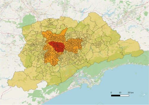
The study area is divided in 633 zones used by the census (which is described further below). This zonal system has been used since the 1970s and is updated regularly. It ensures a rather homogeneous distribution of the population among the zones: in each one, the number of residents is between 20 and 55,000. The HTS, which will be described below, is based on another zonal system that contains fewer zones. As this data set also contains coordinates of all activities, it allows us to impute the census zones for each activity.

Facility locations

Unfortunately, we have not been able to obtain a sufficiently good enterprise census, nor a housing census for São Paulo. While Open Street Maps (OSM) is usually a good source of shopping, leisure, work and home locations, this is not the case for Brazil. To overcome this issue, we placed points on every residential road in order to model facilities that are not present in the OSM data. Educational facilities are obtained from São Paulo’s Ministry of Education. The data set Dados Abertos da Educação Coordenadoria de Informaço, Evidência, Tecnologia e Matrícula (CITEM) (2020) is used. This data set contains the geographical coordinates of all education places in the state of São Paulo, but, unfortunately, the level of offered education is missing.

While the data set is by no means perfect, the modularity of our approach allows one to easily add new sources of information if they become available.

Mobility demand: the population

Two main data sources were used as inputs to create the synthetic demand. The first is a census conducted in 2010 in Brazil.¹ A total of 10% of the Brazilian population was interviewed. After removing all samples that have a home place outside São Paulo State, 3,622,779 weighted samples remained. For each, information is provided on the individual’s age, gender, personal income, employment and/or student status. Plenty of other attributes are available, but they are not used in the present study. There is also access to household-related attributes, such as total household income, car and motorcycle availability, number of household members, and the municipality and zone identifier of the place of residence (Figure 1). Among those individuals, 1,211,311 live in the study area. Their weights sum to 19,918,293, which is approximately the total number of inhabitants in the Greater São Paulo Metropolitan Region at the time the survey was conducted. The census is necessary to make sure that the attribute distributions (whether individual or household related) in the synthetic population fit accurately reality.

The second data source is the Household Travel Survey (HTS) conducted in the Greater So Paulo Metropolitan Region in 2017.² It contains 84,889 person samples, which are weighted so that the total weight accumulates to 20,508,979 inhabitants, which is close to the real total in 2017. For each sample, not only are individual attributes provided (e.g., age, gender, personal income and employment status), but also information related to the household (e.g., income and number of available cars and bikes). The most important part of the survey is the activity sequences, which make it possible to track each interviewed individual’s schedule during an average workday. Each entry corresponds to a trip linking two given activities which take place at locations known at the coordinate level. Moreover, one has access to trip characteristics such as departure and arrival time and chosen mode. Some individuals also answered questions about the type of parking they used and how much they paid for it. Nevertheless, those persons were too few to justify further processing of these information.

Origin– destination commute matrices

An origin–destination (OD) commute matrix is a matrix in which each cell represents the number of trips from an origin zone (given by the corresponding row of the matrix) to a destination zone (column), or the percentage of trips starting in the origin zone that reach the destination zone, for work and education. These matrices are usually provided by government agencies. Unfortunately, this is not the case for Brazil. Therefore, commuting matrices are generated from the HTS. Trips within the same zone are included in those matrices. In this study, a weighted OD matrix was only generated for work trips. For education, the matrix was too sparse (since it had to be generated from the HTS), as will be explained further below.

CREATION OF THE SYNTHETIC TRAVEL DEMAND

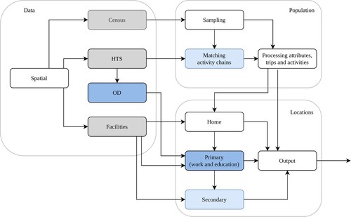
The goal of this section is to present the process leading towards the creation of a synthetic travel demand using the data presented in the previous section. The pipeline is available as a public repository.³ Apart from the framework generating the synthetic travel demand, this repository also provides scripts embedding the travel demand into a transport simulation using MATSim (Horni et al., 2016) and its discrete-mode choice extension (Hörl et al., 2018). Presenting the downstream simulation is beyond the scope of this paper, but further details can be found in the code repository. Figure 2 shows three main stages of the pipeline: Data, Population and Locations. Grey blocks denote stages that have to be adapted for each scenario to guarantee consistently formatted outputs; light blue blocks denote a stage in which the user has to manually choose which attributes are used; and dark blue blocks represent stages for which an implementation specific to São Paulo was proposed.

Figure 2. Overview of the travel demand generation using the eqasim pipeline for São Paulo.

Note: White blocks denote stages for which the standard implementation remained unchanged; light blue blocks are stages where user configuration is required; grey blocks are stages that must be adapted to guarantee consistent outputs; and dark blue blocks are stages for which an implementation specific to São Paulo is proposed.

Pre-processing the input data

While most of the data sets are used in their original form, some of the information from the HTS need to be adapted to reduce complexity. All data sets are processed and prepared in the Data stage. As these data sets can vary across countries, they are in detail described below, and notable differences are highlighted.

Employment, transport mode and trip purpose categories

In the HTS, respondents are allowed to choose among 17 different transportation modes. In order to simplify the modelling tasks, they were merged to eight modes, namely public transport, car, car passenger, walk, bike, taxi and ride-hailing.

For similar reasons, the trip purposes, that is, activity types conducted at the trip destination, are merged into six categories (home, work, shopping, leisure – including entertainment and going to restaurant and bars, education, and other). Those categories can be freely adapted according to the study purposes. It has to be mentioned that trips done by non-studying adults to escort their children to school were initially classified as ‘education’ trips in the original data set. Those activities are adjusted to ‘other’ to avoid potential confusion.

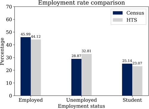
It is also necessary to reduce the number of employment categories from eight to three to guarantee consistency with the classification present in the census. Full- and part-time workers as well as employed persons in long medical leave are considered as ‘employed’, whereas retired individuals, temporarily or long-term unemployed persons and homemakers are classified as unemployed, and the student category remains unchanged.

Comparing HTS with census employment numbers presented a large disparity in the number of unemployed people. Therefore, we performed a check whether those going to school were classified as students using a variable about current school enrolment available in the HTS. While a majority of individuals were correctly classified as student, there were some who were classified as either ‘jobless’ or ‘has never worked’. For these, we adjusted the status of their employment to ‘student’. As a result, the respective shares of students, employed and unemployed individuals in the HTS were closer to that observed in the census (Figure 3). Further discussion of this can be found in the section ‘Comparison of the activity chains’.

Figure 3. Distribution among employed, unemployed and currently studying persons in both the census and the Household Travel Survey (HTS).

Adding residence area information

One’s mobility patterns are influenced by one’s residential environment. For instance, in less densely inhabited zones, a trip tends to be longer than in a highly populated neighbourhood, and car prevalence tends to decrease in the most urbanized areas, mostly due to difficulties of finding (affordable) parking. We capture this phenomenon by creating a new attribute, which splits all individual samples from the census and the HTS into three groups depending on the location of their home. Figure 1 shows the three zones that were defined.

Creating synthetic households

After processing the census and the HTS, we created synthetic households by directly expanding the census households according to their weights within the Census stage. While there are multiple methods in the literature to create synthetic households based on the marginal data (i.e., Chapuis et al., 2018; Ilahi & Axhausen, 2019), here a simple expansion of the census data was possible. The census data are anonymized by providing home locations only by zone, therefore further assignment of the exact home location is performed later in the pipeline.

Assigning activity chains

In the Population part, the Sampling stage can be used to provide a sample of households (i.e., when a user wants to simulate a smaller sample in the downstream agent-based simulation). In our case we maintain all households generated in the Census stage. The Matching activity chains stage then assigns to each individual in the household an activity-chain observation from the HTS, using hot-deck matching (D’Orazio et al., 2012; Hörl & Balac, 2021a).

The idea is to find all HTS persons who match a sampled synthetic individual on a list of attributes, and to randomly select one of them for further processing. We attach the whole activity chain of the selected HTS person to the synthetic individual. To avoid overfitting, the list of matching attributes is sequentially reduced if too few HTS observations (the minimal admissible number of observations is five) are found for an individual.

The configurable attributes that are taken into account to perform matching are age (categorized into 11 classes: 0–6, 7–10, 11–14, 15–18, 19–24, 25–30, 31–42, 43–54, 55–66, 67–78 and > 78 years old), gender, employment status and availability of a car within the household. In addition, observations that are similar with respect to residence area (as defined in reference to the section ‘Adding residence area information’) are preferred. Matching residence area is not mandatory as its influence is already captured by other attributes, notably car ownership.

Imputing primary locations

Once the agents have been assigned a daily plan based on the HTS, a location for each of their activities is defined within the Locations stage. First the location primary activities (home, work and education) must be defined. The aim of this step is twofold: first, the correct number of agents should commute from one zone to another; and second, the commute distances should fit the activity chains that have been assigned to the agents in the previous step. While only an overview of the algorithms will be given in the following, more details can be found in Hörl and Balac (2021a).

Imputing home locations

The assignment of home location happens for each household. The administrative zone in which each agent lives is known from the census and, thus, as all admissible home locations are available from the facility locations database. We impute a home place to each synthesized household by sampling a home place among all available locations in a given zone.

Imputing work locations

We provide individuals with work locations if they have at least one work-related trip registered in their activity chain. For this purpose, the OD matrices are used.

Given the residence district of an agent, their workplace district is sampled from the corresponding line of the weighted OD matrix. For each pair of districts, the number of commuting relations is then known. For each relation, viable destinations from the data set containing all available workplaces are sampled. Additionally, a reference commuting distance between home and work can be derived for every agent from the HTS. Using this information, the destinations are assigned one by one to the agents of a specific relation such that the distance between the synthetic agent’s home location and the sampled destination gets close to that found in the HTS.

Imputing education locations

The imputation of the education locations follows a different path. For the less dense districts, too few observations were registered, which led to biased OD matrices. Moreover, the facility data sets obtained from the Ministry of Education do not provide enough information about the category of education facility (kindergarten, primary, high school or university).

All education-related trips from the HTS are first split into several groups depending, first, on the residence area type (see the section ‘Adding residence area information’) in which the agent lives; second, on the agent’s gender; and, third, on the age of the individual who performed the trip and thus on the category of education facility the individual visited: pre-school or elementary school for children aged ≤ 14, high school or technical school for teenagers aged 14–18, university for people aged 18–30, and various places for agents aged ≥ 30. For each of these groups, we construct the histogram of the distances separating the place of education to the home of the individual samples, based on the crow-fly distances between the place of residence and the education facility reported in the HTS. Finally, a probability density function corresponding to each histogram is obtained. This method ensures that each student travels an appropriate distance between their home and the place where they study; however, the corresponding flows between the census zones might not be respected.

For each agent, a target distance is drawn from the probability function related to the group (age and type of residence area) to which the agent belongs. Using a bidimensional k-d tree, an education place is then selected such that the distance separating it from the agent’s home location was as near to the target distance as possible.

Imputing secondary locations

The imputation of secondary locations, which means places in which leisure, shopping or other activities are performed, is accomplished by the method described by Hörl and Axhausen (2020) or, more briefly, by Hörl and Balac (2021a). Only a basic idea will be given here so as to provide some intuition on the employed algorithm.

While primary activities (home, work or education) have fixed locations, which were determined in the previous steps, secondary activities (shopping, leisure and other) are not yet assigned particular locations. The activity chains can be split into smaller chains in which two fixed activities, the first and last ones, are separated only by various assignable activities. From the HTS, one knows how long the trips of each sub-chain should ideally be.

First, all trips present in the HTS are divided into bins of modes and travel times. Given the transport mode and the HTS travel time of each trip, a distance is then sampled from the bins previously created. Afterwards, a gravity model is used to assign the variable activities along a chain to locations, defined by coordinates, such that the resulting distances resemble the sampled ones. Finally, the closest facility of the target activity type is selected from the facility data sets for each location. For instance, if an agent goes ‘shopping’, the sampled coordinates are snapped to the nearest available shop.

This approach guarantees that agents travel a realistic distance to perform their secondary activities. However, currently one drawback of the algorithm is that it takes into account neither the facilities’ capacity nor the exact type of activity they offer. Therefore, in situations where these data are available, further improvements of the algorithm becomes valuable.

The output’s structure

At the end of the travel demand synthesis, several files are created. Regarding the population, one file describes the household by two attributes (monthly income, residence area and car ownership) and another summarizes key individual attributes (gender, age, employment status, driving licence and transit subscription). Regarding the mobility patterns, one file summarizes all activities performed by the synthetic population – one knows which individual performed the activity and when, and which activity it was – and the last one contains information (departure and arrival time, mode, preceding and following purpose) about all trips done. Of course, all those files can be adapted depending on the purpose of the study.

INSIGHTS INTO THE SYNTHETIC TRAVEL DEMAND

The process described above enables the creation of a synthetic travel demand in which the agents are given activity chains obtained from the HTS and where those activities are performed in places drawn with various sampling methods from the facility databases.

The fact that the census is very accurate, and that the synthetic agents and households are directly sampled from this data set, leads to the conclusion that a validation step to assess the accuracy of the socio-demographic attributes distribution in the synthetic population is not necessary. This is why this point will not be addressed below.

Comparison of the activity chains

Figure 4 shows the distribution of activity chains in the synthetic population and compares it with the observed distribution obtained from the HTS. The graph suggests that the synthesis process provides a good match, which is confirmed by a Spearman’s rank-order correlation coefficient of 0.81 (p <0.01). However, it can be seen that chains containing at least one ‘work’ activity (such as ‘h-w-h’ or ‘h-w-l-w-h’ in Figure 4) are more frequent in the synthetic travel demand than in the HTS. The reason for this is that the two surveys used in this study were not conducted in the same year. The distribution among the three employment categories – namely ‘employed’, ‘unemployed’ (which includes retired people as well) and ‘student’ – changed during the seven years separating the time when the census was conducted (in 2010) and the period at which the HTS was realized (in 2017) (Figure 3).

Figure 4. Activity chains comparison.

Note: h, Home; w, work; e, education; l, leisure; s, shopping; and o, other.

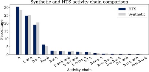
The employment rate as well as the percentage of students in the population dropped between 2010 and 2017. This is why the plans containing one or more work or education activities are slightly over-represented. Moreover, for the same reason, the number of agents who do not leave their home (those whose activity chain is only ‘h’) tends to be higher in the HTS than in the census, and thus in the synthetic travel demand. Official sources confirm the quite dramatic rise in unemployment in São Paulo: the unemployment rate was around 7% in 2010 (Instituto Brasileiro de Geografia e Estatística (IBGE), 2016) in the metropolis, and increased to 13.4% in 2017 (IBGE, 2017).

Comparison of the trip distance distributions

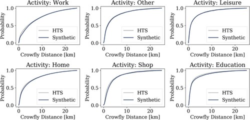
Comparing how far agents have to travel to perform a given activity with what is observed in reality can help us to understand the quality of the activity location assignment process. The results of this comparison are presented in Figure 5; it shows that the distance distributions fit very satisfactorily.

Figure 5. Distributions of crow-fly distances towards a facility, by activity purpose.

Comparison of travel purposes and distances between male and female agents

As described in the previous section, the activity chains present in the HTS are correlated with the socio-demographic attributes of the interviewees and, thanks to the matching process, those chains are distributed in a meaningful way among the synthetic agents. Figure 6 compares the prevalence of the most frequent activity chains in the HTS and the synthetic travel demand for male and female agents between 18 and 40 years of age. It shows that the chain ‘h-w-h’ (going from home to work and then back home) is the most prevalent for both agents groups, but in the HTS as well as in the synthetic travel demand, the observed frequency among males is more than 10 percentage points above the frequency observed among female agents (42–45% versus 55–57%). As a consequence, the chain distribution observed for women seems to be slightly more heavy-tailed than that characterizing men.

Figure 6. Most frequent activity chains: comparison between the Household Travel Survey (HTS) and synthetic travel demand, split between men and women aged 18–40 years.

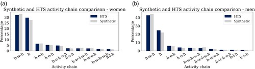
This indicates a larger variety of activity patterns for women, a phenomenon that has already been investigated by Scheiner and Holz-Rau (2017). This observation is confirmed by Figure 7, which shows the number of activities and, alternately, the number of activities per purpose in the HTS and the synthetic travel demand for male and female individuals aged between 18 and 40 years.

Figure 7. Number of activities in the chains (top row) and number of activities per purpose (bottom row): comparison between the Household Travel Survey (HTS) and synthetic travel demand, split between men and women aged 18–40 years.

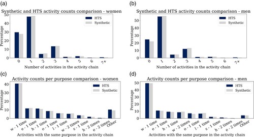
It can also be noticed that the fifth most prevalent activity chain is different between the male and female populations: it is indeed ‘h-w-h-w-h’ for men and ‘h-o-h-o-h’ for women. A further analysis reveals that this chain was originally ‘h-e-h-e-h’ for women; those ‘education’ activities were adjusted into ‘other’ ones during the cleaning part as they represent pick-up and drop-off activities. This difference in the activity chain distribution among men and women thus reflects an activity splitting among household members: women who stay at home take care of the children, whereas men are more often employed and some of them return home for lunch.

DISCUSSION

Input data

The available input surveys (the census and the HTS, conducted in 2010 and 2017, respectively) were not carried out in the same year. During the period separating them, the population structure evolved in many aspects. The ‘unemployment’ rate (each person who is neither employed nor a student is here considered unemployed) rose by 6 percentage points between 2010 and 2017. The observed mobility patterns were influenced by the latest developments of the public transport network (such as the construction of new metro lines⁴ or the start of operations of ride-hailing platforms, such as Uber in June 2014, as reported by Zanatta & Kira, 2018).

Travel demand was thus synthesized from two temporally distinct data sets. This is why synthetic mobility patterns sometimes do not match precisely those taken as a reference. Potentially, one could either wait for new census data to be published or update the census information based on information in the HTS to represent the present socio-demographic characteristics better. Moreover, the HTS only allows one to model usual personal trips. While own-account logistics is captured through the HTS, neither freight nor tourism travel patterns are considered. Therefore, this could have consequences on the global accuracy of the downstream agent-based simulation and on its ability to assess the transport situation in the metropolis on an average day.

Facilities’ locations

A few issues have arisen concerning the creation of the facility data sets. For instance, as OSM does not have adequate representation of education locations in the region, the first attempt to assign education places to the synthetic individuals ended up being erroneous. The distribution of the individuals’ distances to reach their study location starting from their home was too dissimilar to the target distribution. This highlights the importance of having access to high-quality input data. To overcome this issue, it was possible to use a data set provided by São Paulo’s Ministry of Education. However, this was not possible for other activity categories, such as leisure, shopping or housing.

Further improvements

As pointed out above, there is still room for improvement, which would lead to more accurate results and better representation of the average mobility demand in the São Paulo Metropolitan Region. Most of it has to do strongly with data availability:

• As mentioned in the introduction, Santos is a major city with a population of more than 400,000 inhabitants. Being home to the largest seaport of Latin America, located only 80 km from São Paulo, it is apparent that it contributes to transport flows in the megacity. In particular, taking into account commuter flows from one city to the other would enhance the travel survey and, as a result, improve the quality of the modelled transport demand.

• Freight traffic and commercial agents’ routes are also missing in the current trips data sets. As the impact of such trips may not be negligible on the global transport situation, taking them into account would benefit later transport simulation.

• Currently, in the process of matching activity chains to individuals, the household structure is not considered. As all household members are interviewed in the HTS, it would be possible to maintain the interactions existing within the households in the matching phase. This would ensure that joint trips are appropriately modelled, and that shared resources (cars or bicycles, for instance) are distributed appropriately among the household members.

Integration into an agent-based model

One of the goals of producing such a travel demand is its integration into a full agent-based model. The transport supply has to be created and added to the travel demand to obtain a complete transport scenario. OSM data (e.g., based on a regional cut-out from Geofabrik⁵) can be used to create the network in the study area, based on open data. Transit schedules (or General Transit Feed Specification, GTFS) are obtained from public transport operators. Then, both demand and supply can serve as the basis for transportation simulations to ultimately conduct policy analysis studies. While this process is available and documented within the same Github repository, it is beyond this paper’s scope.

CONCLUSION

This paper presented a process to generate a synthetic travel demand for São Paulo, based on the eqasim framework allowing, among other components, one to obtain an operational agent-based model directly from the raw data. All the data sets used here and the framework are open source, and, consequently, the results are entirely reproducible by others.

Based on straightforward algorithms, the proposed approach can be easily adapted to the generation of other scenarios. It could, therefore, serve as a benchmark for future improvements. It also shows that reliable outputs can be obtained even if the input data are not the most suitable – in the case at hand, the census data were collected seven years before the HTS was conducted. Even though not methodologically novel, it should be emphasized that, to the authors’ knowledge, it is the first-ever travel demand synthesized for São Paulo and, more generally, for Brazil that can be directly employed in agent-based models to conduct numerous studies.

Possible improvement axes for future study include freight traffic, commuter flows from and to Santos, or household structure during the matching of activity chains phase. The hope is to continue to collect data and to expand this approach to new scenarios. As the presented approach is open source and based on open data, its results are available to anyone. This fosters and encourages accessibility and reproducibility of scientific tools and findings.

DISCLOSURE STATEMENT

No potential conflict of interest was reported by the authors.

Additional information

Funding

The authors acknowledge Airbus Urban Mobility GmbH whose funding supported the development of a synthetic agent-based scenario for the Greater São Paulo Metropolitan Region.

Notes

1 See https://www.ibge.gov.br/en/statistics/social/population/18391-2010-population-census.html?edicao=19720&t=sobre/.

2 See http://www.metro.sp.gov.br/pesquisa-od/.

3 See https://github.com/eqasim-org/sao_paulo/.

4 See http://g1.globo.com/sao-paulo/noticia/2014/08/primeiro-trecho-da-linha-15-prata-do-monotrilho-e-aberto-em-sao-paulo.html (accessed July 15, 2021).

5 See https://download.geofabrik.de/.

REFERENCES

- ActivitySim (2020). An open platform for activity-based travel modeling. URL https://activitysim.github.io/.
- Axhausen, K. W., & Gärling, T. (1992). Activity-based approaches to travel analysis: Conceptual frameworks, models, and research problems. Transport Reviews, 12(4), 323–341. https://doi.org/https://doi.org/10.1080/01441649208716826
- Balac, M., Ciari, F., & Axhausen, K. W. (2015). Carsharing demand estimation: Case study of Zurich area. Transportation Research Record, 2536(1), 10–18. https://doi.org/https://doi.org/10.3141/2536-02
- Balać, M., & Hörl, S. (2021, January). Synthetic population for the state of California based on open-data: examples of San Francisco Bay area and San Diego County. 100th Annual Meeting of the Transportation Research Board, Washington, DC, USA.
- Bischoff, J., & Maciejewski, M. (2016). Simulation of city-wide replacement of private cars with autonomous taxis in Berlin. Procedia Computer Science, 83, 237–244. https://doi.org/https://doi.org/10.1016/j.procs.2016.04.121
- Bowman, J. L. (1995). Activity based travel demand model system with daily activity schedules [Doctoral dissertation]. Massachusetts Institute of Technology.
- Bowman, J. L. (1998). The day activity schedule approach to travel demand analysis [Doctoral dissertation]. Massachusetts Institute of Technology
- Chapin, F. S. (1974). Human activity patterns in the city: Things people do in time and in space, volume 13. Wiley-Interscience.
- Chapuis, K., Taillandier, P., Renaud, M., & Drogoul, A. (2018). Gen*: a generic toolkit to generate spatially explicit synthetic populations. International Journal of Geographical Information Science, 32(6), 1194–1210. https://doi.org/https://doi.org/10.1080/13658816.2018.1440563
- Chu, Z., Cheng, L., & Chen, H. (2012, August 3–6). A review of activity-based travel demand modeling. In CICTP 2012: Multimodal transportation systems: Convenient, safe, cost-effective, efficient, Beijing, China (pp. 48–59).
- Coordenadoria de Informaço, Evidência, Tecnologia e Matrícula (CITEM) (2020). Endereços de escolas (addresses of the schools). URL https://dados.educacao.sp.gov.br/dataset/endere%C3%A7os-de-escolas.
- de Dios Ortúzar, J., & Willumsen, L. G. (2011). Modelling transport (4th ed.). John Wiley & Sons.
- Diogu, W. O. (2019). Towards the implementation of an activity-based travel demand model for emerging cities: Integrating TASHA and MATSim [Master's thesis]. University of Toronto, Canada. https://www.proquest.com/dissertations-theses/towards-implementation-activity-based-travel/docview/2323546171/se-2?accountid=27229
- D’Orazio, M., Di Zio, M., & Scanu, M. (2012, May, 29–June 1). Statistical matching of data from complex sample surveys. Proceedings of the European Conference on Quality in Official Statistics-Q2012, volume 29.
- Erath, A., Fourie, P. J., van Eggermond, M. A., Ordonez Medina, S. A., Chakirov, A., & Axhausen, K. W. (2012). Large-scale agent-based transport demand model for Singapore. Arbeitsberichte Verkehrs- und Raumplanung, 790.
- Hägerstrand, T. (1970). What about people in regional science? In Papers of the regional science association (Volume 24, pp. 6–21). John Wiley & Sons.
- Hörl, S., & Axhausen, K. W. (2020, January 12–16). Relaxation–discretization algorithm for spatially constrained secondary location assignment. 99th Annual Meeting of the Transportation Research Board.
- Hörl, S., & Balac, M. (2021a). Synthetic population and travel demand for Paris and Île-de-France based on open and publicly available data. Transportation Research Part C: Emerging Technologies, 130, 103291. https://doi.org/https://doi.org/10.1016/j.trc.2021.103291
- Hörl, S., & Balac, M. (2021b). Introducing the eqasim pipeline: From raw data to agent-based transport simulation. Procedia Computer Science, 184, 712–719. https://doi.org/https://doi.org/10.1016/j.procs.2021.03.089
- Hörl, S., Balac, M., & Axhausen, K. W. (2018). A first look at bridging discrete choice modeling and agent-based microsimulation in matsim. Procedia Computer Science, 130, 900–907. https://doi.org/https://doi.org/10.1016/j.procs.2018.04.087
- Hörl, S., Becker, F., Dubernet, T., & Axhausen, K. W. (2019). Induzierter Verkehr durch autonome Fahrzeuge: Eine Abschtzung (traffic induced by autonomous vehicles: An estimation). SVI 2016/001, Schriftenreihe, 1650.
- Horni, A., Nagel, K., & Axhausen, K. W. (2016). The multi-agent transport simulation MATSim. Ubiquity Press.
- Ilahi, A., & Axhausen, K. W. (2019). Integrating Bayesian network and generalized raking for population synthesis in Greater Jakarta. Regional Studies, Regional Science, 6(1), 623–636. https://doi.org/https://doi.org/10.1080/21681376.2019.1687011
- Instituto Brasileiro de Geografia e Estatística (IBGE). (2016). Principais destaques da evoluç ao do mercado de trabalho nas regi oes metropolitanas abrangidas pela pesquisa (Main highlights of the evolution of the labor market in the metropolitan regions covered by the survey). URL ftp://ftp.ibge.gov.br/Trabalho_e_Rendimento/Pesquisa_Mensal_de_Emp%rego/Evolucao_Mercado_Trabalho/retrospectiva2003_2011.pdf.
- Instituto Brasileiro de Geografia e Estatística (IBGE). (2017). Pesquisa nacional por amostra de domicílios contínua – quarto trimestre de 2017 (national household sample survey – fourth quarter 2017). URL https://biblioteca.ibge.gov.br/visualizacao/periodicos/2421/pnact_2017%_4tri.pdf.
- Kitamura, R. (1988). An evaluation of activity-based travel analysis. Transportation, 9–34.
- Lee, Y., Hickman, M., & Washington, S. (2007). Household types and structure, time–use pattern, and trip-chaining behavior. Transportation Research Part A: Policy and Practice, 41(10), 1004–1020. https://doi.org/https://doi.org/10.1016/j.tra.2007.06.007
- Lopez, P. A., Behrisch, M., Bieker-Walz, L., Erdmann, J., Flötteröd, Y.-P., Hilbrich, R., Lücken, L., Rummel, J., Wagner, P., & Wießner, E. (2018, November 4–7). Microscopic traffic simulation using sumo. 2018 21st International Conference on Intelligent Transportation Systems (ITSC) (pp. 2575–2582). IEEE.
- Mallig, N., Kagerbauer, M., & Vortisch, P. (2013). Mobitopp – A modular agent-based travel demand modelling framework. Procedia Computer Science, 19, 854–859. https://doi.org/https://doi.org/10.1016/j.procs.2013.06.114
- Recker, W. W. (1995). The household activity pattern problem: General formulation and solution. Transportation Research Part B: Methodological, 29(1), 61–77. https://doi.org/https://doi.org/10.1016/0191-2615(94)00023-S
- Scheiner, J., & Holz-Rau, C. (2017). Women’s complex daily lives: A gendered look at trip chaining and activity pattern entropy in Germany. Transportation, 44(1), 117–138. https://doi.org/https://doi.org/10.1007/s11116-015-9627-9
- Viegas, J. M., & Martínez, L. M. (2010, July 11–15). Generating the universe of urban trips from a mobility survey sample with minimum recourse to behavioural assumptions. Proceedings of the 12th World Conference on Transport Research, Lisbon.
- Wen, C.-H. (1998). Development of stop generation and tour formation models for the analysis of travel/activity behavior.
- Zanatta, R. A., & Kira, B. (2018). Regulation of Uber in Sao Paulo: From conflict to regulatory experimentation. International Journal of Private Law, 9(1–2), 83–94. https://doi.org/https://doi.org/10.1504/IJPL.2018.097332
- Ziemke, D., Kaddoura, I., & Agarwal, A. (2019b). Entwicklung eines regionalen, agentenbasierten Verkehrssimulationsmodells zur Analyse von Mobilitätsszenarien für die Region Ruhr. In Mobilität in Zeiten der Veränderung (pp. 383–410). Springer.
- Ziemke, D., Kaddoura, I., & Nagel, K. (2019a). The MATSim Open Berlin Scenario: A multimodal agent-based transport simulation scenario based on synthetic demand modeling and open data. Procedia Computer Science, 151, 870–877. https://doi.org/https://doi.org/10.1016/j.procs.2019.04.120
- Ziemke, D., Nagel, K., & Bhat, C. (2015). Integrating CEMDAP and MATSim to increase the transferability of transport demand models. Transportation Research Record, 2493(1), 117–125. https://doi.org/https://doi.org/10.3141/2493-13