Empirical methods in business location research

ABSTRACT

A frequent theme in regional science is exploring the determinants of business establishment locations. We briefly review the theoretical perspectives motivating several frameworks underpinning locational determinant analyses. We summarize and review trade-offs involved in established and emerging econometric techniques that researchers use to analyse locational determinants. We conclude with opportunities for future research, including understudied frameworks, potential data sources and methodological developments.

KEYWORDS:

• business location
• econometric models
• count data
• administrative data

JEL CLASSIFICATIONS:

• C18
• R12
• R3
• R53
• R58

INTRODUCTION

A theme of regional economic research is the determinants of business location, relocation, creation, attraction, retention, expansion or ‘firm demography’ (Pellenbarg et al., 2002). In the United States, studies document the decline in establishments’ birth rates since the 1990s and examine the negative effects on economic growth therefrom (Gourio et al., 2016; Haltiwanger et al., 2013).¹ In other high-income economies, inward investment policy, also known as industrial recruitment, is an area of active research (Raganowicz, 2018; Rutherford et al., 2018; Tewdwr-Jones & Phelps, 2000; Xu et al., 2020). While reviews have been published (Dicken & Lloyd, 1990; Iammarino & McCann, 2013; Krugman, 1995; McCann, 2002a; McCann & Sheppard, 2003; Pellenbarg et al., 2002; Shaffer et al., 2004) on the empirical results of industrial location studies (Arauzo-Carod et al., 2010; Blair & Premus, 1987; Daniels, 1985), and on broader combinations thereof (Balbontin & Hensher, 2019; Fujita et al., 1999; Goetz et al., 2009; Hayter, 1997), the present article provides a review of empirical methods for assessing business locational determinants. It offers a practical guide on the choice of empirical methods under different data options. Though the article includes a brief overview of locational theoretical perspectives and their underlying frameworks, the purpose of the theory section is only to provide a contextual framework in which the empirical methods operate.

Regarding data, this article highlights that most of the business location literature, particularly from the demand threshold perspective, measures industry size by the number of establishments within an industry and region (Goetz et al., 2009). While this approach is logical for some service industries where establishments function as nodes of service, the consolidation of other industries supports the argument that more detailed measures, such as employment or payroll, could be more accurate.

Although this article focuses on empirical approaches and data issues relevant to business location research, analytical frameworks can inform those approaches; hence, the next section briefly reviews the theoretical perspectives and frameworks on locational determinants, providing a taxonomy of the frameworks and underpinning theory. Next, informed by the interacting data issues (in the third section), this article reviews the evolution of empirical methods (in the fourth section). Concluding with opportunities for future research, we highlight underused data sources that may facilitate improvements in locational determinant research: the analysis of understudied frameworks, enhanced measurement of industry size and development of spatial count data models.

ANALYTICAL PERSPECTIVES ON LOCATIONAL DETERMINANTS

Analytical perspectives include: (1) demand thresholds and (2) spatial monopsony, which both stem from central place theory (Berry & Garrison, 1958a, 1958b; Christaller, 1966; Lösch, 1954); (3) classical and neoclassical location–production models (Weber, 1909); (4) New Economic Geography (NEG) (Krugman, 1991a, 1991b, 1995); and (5) firm demography (van Dijk & Pellenbarg, 2000), which includes the (5.1) random profit maximization (McFadden, 1973), (5.2) behavioural and (5.3) institutional frameworks.² While the latter two frameworks receive less attention, we include them because new data and empirical techniques make implementation increasingly feasible (Conroy et al., 2016; McCann, 2002a; Pellenbarg et al., 2002).

Demand threshold framework

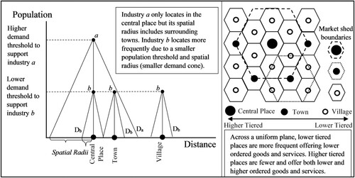
Demand threshold analysis relies on Central Place Theory (CPT), which predicts that the determinants of a good’s range are both the cost of supplying the good and the demand for the good (Christaller, 1966; Lösch, 1954). A demand threshold is the minimum market size required to support a type of service business that still yields a rate of return greater than the owner’s reservation wage (Berry & Garrison, 1958b, 1958a; Harris et al., 1996; Parr & Denike, 2016; Shaffer et al., 2004). Spatial equilibrium occurs when the revenue under the demand structure covers operating costs and allow an acceptable rate of return. Past research confirms differences in demand thresholds across industries (Shonkwiler & Harris, 1996), and can advise decision-makers on the potential feasibility of new establishments in an area (Wensley & Stabler, 1998). We provide the classic graphical representation of demand thresholds in Figure 1 (see also Carpenter et al., 2021a).

Figure 1. Simple graphical representation of the demand threshold framework.

Source: Authors, drawing on Christaller’s (1966) classic work.

Spatial monopsony framework

Spatial monopsony also draws on CPT. Under spatial monopsony, competition of an establishment handling dispersed raw material input occurs on the edges of the market shed, rather than within a central place. The spatial monopsonist faces an upward-sloping cost curve as it expands its territory, classically due to transportation costs associated with bringing raw product to a processing facility. Parr and Swales (1999) show an array of circular markets with spaces of the familiar CPT honeycomb network unserved, except at the points where the service area circle is tangent to the edge of the hexagon, and the outer radius of the adjoining competitor’s market shed. The question of spatial price competition is an important theme in agricultural markets (Li et al., 2018; Sesmero et al., 2015).

Location–production models

Also involving profit maximization, location–production models analyse the relationship between geography and production behaviour, specifically how optimal input levels are related to spatial costs (McCann, 1995). The classical location–production model (Weber, 1909) emphasizes the roles of the input–output structure of a firm’s production function and transportation costs on the firm’s optimal location. This model is generalizable to allow for input substitution (allowing a role for input prices) in the co-determination of input combinations and firm locational choice (Moses, 1958). McCann (1996) further expands this framework to allow for market prices, revenue and distance costs to play a role. These frameworks do not allow spatial variation in local land and labour prices (McCann, 2002b).

New Economic Geography (NEG)

NEG (Krugman, 1991a, 1991b, 1993, 1995) starts with industrial agglomeration stemming from a trade-off between external economies of scale and transportation costs, but also analyses agglomeration effects as developing into a system of cities as an endogenous process. That is, the economy is divided into n possible locations and two industries: one industry is immobile in production and the other can choose its optimal location. With labour as the production factor, labour supply fixed and workers as the consumers, the geographical distribution of labour over the locations equals that of production. A long-run equilibrium is reached when real wages in all locations have become equal and no more migration of manufacturing workers occurs. The model tends toward self-reinforcing agglomeration. As Krugman (1993, 293) writes, ‘the eventual locations of cities tend to have a roughly central-place pattern’. As noted above, Mulligan et al. (2012) remark that CPT’s multiple regional concepts and interplay between consumer choice, agglomeration, and a functional hierarchy of places make it a complement to NEG models, rather than a competitor.

Firm demography

The firm demography perspective accounts for a firm’s birth (start-up), merger, splitting, migration (relocation) and death (closure) (Hoogstra & van Dijk, 2004; Pellenbarg et al., 2002; van Dijk & Pellenbarg, 2000). Firm demography accommodates neoclassical, behavioural and institutional approaches (Machlup, 1967).

Neoclassical profit maximization

Firm demography is an analytical framework in which we place neoclassical profit maximization, but the classical approach dates back to Adam Smith (Isard, 1956). Modelling a firm’s locational choice has a long history spawning from McFadden’s (1973) discrete choice work, with ongoing work examining the effect of various local factors influencing profitability (Bartik, 1985; Carlton, 1983). Manufacturing location decisions do not typically rely on the demand-side considerations central to CPT, but rather on the profit maximization (and cost minimization) (McCann, 2002a).³

The neoclassical conception of locational choice follows McFadden (1973) and considers the relative profits, ${\pi }_{ij}$, for establishment $i\in \{1,2,\dots ,I\}$ resulting from locating in geography $j\in \{1,2,\dots ,J\}$. An establishment’s profit results from a linear combination of a deterministic term, ${\tilde{\pi }}_{ij}$, and stochastic term, ${\epsilon }_{ij}$, such that: ${\pi }_{ij}={\tilde{\pi }}_{ij}+{\epsilon }_{ij}.$Modelling ${\tilde{\pi }}_{ij}$ as a linear combination of the explanatory variables: ${\tilde{\pi }}_{ij}=X\beta +Z\delta$where $X$ is a matrix of location-specific variables (e.g., amenities, taxes, local institutions, other local policies); and $Z$ is a matrix of industry location-specific variables (e.g., labour costs, other input costs, agglomeration economies). If modelling multiple industries simultaneously, the linear combination can include an additional vector of industry-specific variables (e.g., entry barriers).⁴

Geography $j$ is thus chosen by establishment $i$ if: ${\pi }_{ij}>{\pi }_{ik},\mathrm{\forall }k\ne j.$The stochastic nature of ${\pi }_{ij}$ produces the probability of establishment $i$ locating in geography $j$: $P_{ij}=P({\pi }_{ij}>{\pi }_{ik}),\mathrm{\forall }k,k\ne j.$Assuming independent and identically (extreme value Type I) distributed errors leads to the conditional logit model form: $P_{ij}={\displaystyle \frac{e^{{\tilde{\pi }}_{ij}}}{{\sum }_{k=1}^K{e}^{{\tilde{\pi }}_{ik}}}.}$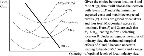We provide the classical graphical representation of random profit maximization in Figure 2.

Figure 2. Simple graphical representation of random profit maximization.

Behavioural framework

The behavioural framework, where profit maximization is not the goal (Cyert & March, 1963; Simon, 1955), is less studied. Apart from alternative goals in the decision-making process, there are four elements in behavioural location theory: (1) the role of limited information; (2) the ability to use information; (3) perception and mental maps; and (4) uncertainty (McCann, 2002a). Nonetheless, this is an important area for future research; with inequity among race, ethnicity, gender and other business-owner characteristics affecting numerous business outcomes (Carpenter & Loveridge, 2018, 2019, 2020). It stands to reason that locational determinants would also be affected. Hence, leaving entrepreneur idiosyncrasies to ${\epsilon }_{ij}$, as in the random profit maximization framework, may bias estimates, or make estimates only representative for majority groups.

Institutional framework

The institutional framework (McNee, 1958) emphasizes the role of existing institutions, such as governments, real estate brokerage services, small business development centres or regional economic development organizations, among others. Both the institutional approach and the neo-classical approach are more applicable to large companies possessing negotiating power, because a decision to move is viewed as a result of negotiations with the community, local government and suppliers, as well as other economic and social actors (Brouwer et al., 2004; Conroy et al., 2016). Factors most relevant to the institutional framework are difficult to quantify, which has limited the development of a well-established empirical literature; nonetheless, there are exceptional articles using the institutional framework (Guimarães et al., 1998; Lee, 2008; Oukarfi & Baslé, 2009) and more detailed reviews (Hayter, 1997; Scott, 2000).

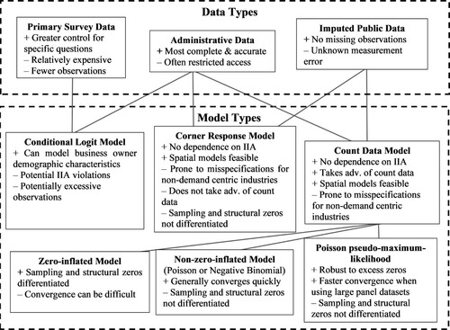
DATA SUMMARY

This section reviews data issues and data sources before the methodology section because data limitations informed the evolution of methods in the locational determinant literature. For example, geography–industry-aggregated data are commonly released by statistical organizations to prevent improper disclosure. Thus, researchers often measure industry size in a location with establishment counts, which includes numerous zeros and is a non-negative integer count, $y\in \{0,1,2,3,\dots \}$. Resultantly, modelling efforts often draw on ‘corner response at zero’ estimators, conditional logit and count data estimators (Wooldridge, 2010). Limitations on these approaches result from disclosure issues and because a local count of establishments is an imprecise proxy for local industry size. More detailed measures of industry size, such as employment, may change the results (Carpenter et al., 2021a; Van Sandt et al., 2021a). Referring to Figure 1, these errors or ambiguous measures of industry size create ambiguous demand thresholds which may be visually depicted as wide bands rather than a line pertaining to a point estimate. Further, establishments of ambiguous size may be characterized by banded spatial demand cones and ambiguous market radii.

Similarly, for cost-centric industries and referring to Figure 2, the estimated marginal effects of X and Z become uncertain, leading to banded Marginal Cost (MC) curves, a range of optimal industry sizes for each location and less confidence in the preferred location. This issue is particularly relevant for consolidating industries where total employment has been stable. Examining employment or payroll as alternative measures of industry size is thus an area for future research.

With public US county-level data, researchers often resort to imputing suppressed cells or using proprietary datasets of unknown accuracy and methods; imputation methods vary widely and include simply using the midpoint of size classes (Autor et al., 2013; Glaeser et al., 1992; Porter, 2003).⁵ Given the unknown error with suppressed-cell estimated datasets (SCEDs), there is a history of efforts to improve SCEDs over the midpoint technique (Isserman & Westervelt, 2006; Orr & Buongiorno, 1989). Researchers who use SCEDs often do not document methods used to produce the estimates (Anselin et al., 1997; Gerking & Isserman, 1981; Isserman, 2001; Markusen, 1996), which may substantially bias coefficient estimates (Carpenter et al., 2021b). Additionally, researchers often resort to using relatively aggregated industries due to disclosure limitations, which can cause aggregation bias (Carpenter et al., 2021c).

Detailed unsuppressed microdata are available in the United States in the Federal Statistical Research Data Center (FSRDC) system. In Europe, Eurostat similarly offers detailed longitudinal data (Eurostat, 2020). Researchers are already using many of these sources of detailed longitudinal establishment-level data to examine firm establishment location decisions (Arauzo-Carod & Viladecans-Marsal, 2009; Devereux et al., 2007; Figueiredo et al., 2002; Holl, 2004; Van Sandt et al., 2021a).

In the United States, the Longitudinal Business Database (LBD) is an annual Census Bureau series (Jarmin & Miranda, 2002). The LBD is a valuable dataset for researching the determinants of entry, growth and exit at the establishment, firm and industry levels (Carpenter & Loveridge, 2019; Haltiwanger et al., 2013). The LBD is commonly used in business research generally, but has not been used as often when examining the determinants of business locational choice (Becker & Henderson, 2000). The LBD combined with the Annual Business Survey (formerly the Survey of Business Owners) has potential to greatly strengthen behavioural research that includes interest in characteristics of the owner.

Georeferenced data also provide opportunities for more geographically nuanced analyses into establishment location decisions by pairing them with other similarly georeferenced data (e.g., raster-level data) or using geostatistical software to create covariates such as distances to transportation infrastructure, or a function of some specific metric within a defined spatial radius (e.g., count, average, minimum, etc.). For example, the LBD may be linked with the parent Business Register dataset to access every business’ street address; however, geostatistical software options are limited in the FSRDC environment, limiting the utility of georeferenced micro-data. As a related example, in Europe, Bureau van Dijk offers datasets such as Amadeus and Orbis, georeferenced datasets of companies (e.g., Chen & Moore, 2010; Holl & Mariotti, 2018). There are many other purchasable private micro-datasets in Europe, North America and elsewhere, but such geographically rich data can be costly. Examples of business location research using georeferenced datasets include location choices of franchises in Brazil (Bitti et al., 2019), retail co-location in Sweden (Larsson et al., 2014) and a discrete-choice model of business location decisions in Canada (Dubé et al., 2016).

EMPIRICAL METHODS

Data availability informs the choice of empirical method (Figure 3), which has evolved with advances in estimation techniques. Carlton (1983) and Bartik (1985) were among the early adopters of using the multinomial logit procedure (McFadden, 1973; see also Carpenter et al., 2021a). However, researchers noted that the using multinomial logit is imperfect in cases of an excessive number of alternatives, as well as the likelihood that the independence of irrelevant alternatives (IIA) assumption does not hold, given the location alternatives are likely correlated, even when conditioning on observables. Efforts to address these limitations include aggregating alternatives reduce the number of alternatives and introducing spatial group indicator variables (Bartik, 1985).⁶ Nonetheless, these limitations led to the use of nested logit with a smaller alternatives set randomly drawn from the full alternatives set (Friedman et al., 1992; Hansen, 1987). The nested logit still faces limitations both in the imposition of an arbitrarily limited and hierarchical choice set on firms, and the loss in sample size more generally. Finally, both approaches still rely on the IIA assumption within subsets of the alternatives for consistency. Nonetheless, with increasing computing power, logit approaches may be useful for studies using the institutional or behavioural frameworks and microdata.

Figure 3. Business location modeling decision tree.

Note: This figure visualizes the interaction between data types and the associated feasible model types. For more detailed discussion of the additional interaction and overlay of the potential for spatial models/effects, see Table 2. ADV, advantage; and IIA, independence of irrelevant alternatives.

Corner response models

While the nature of establishment and employment data, $y\in \{0,1,2,3,\dots \}$, indicates the use of count data models might be preferable for empirical estimation, a linear model would estimate the average partial effects consistently. That is, consistency holds even though $y_i\ge 0$ and $\mathrm{P}(y_i=0)>0$ (Wooldridge, 2010). However, practical problems with estimating a linear model for non-negative count data include negative fitted values and the assumption of a mean linear in x because $\mathrm{E}(y|x)$ cannot truly be linear in $x$.

One could also use non-count corner response at zero estimators, in which the dependent variable is non-negative, continuous above zero and has a lot of observations at zero (Wooldridge, 2010). For example, some research uses the Type I Tobit (T1T), that is, the standard censored regression model (Tobin, 1958), for firm locational choice analysis (Hastings & Goode, 1982; Hines, 1996), and demand threshold analysis (Harris & Shonkwiler, 1997; Mushinski & Weiler, 2002).⁷ However, the partial effects of an explanatory variable on $\mathrm{P}(y_i>0|x)$ and $\mathrm{E}(y|x,y>0)$ must have the same signs in T1T (Wooldridge, 2010). It is easy to imagine scenarios in which this does not hold. For example, a region with low population may increase the likelihood of some industries locating there, but further reducing the population may decrease the size of that industry in a particular area.⁸ Additionally, the ratio of the partial effects of explanatory variables on $\mathrm{P}(y_i>0|x)$ and $\mathrm{E}(y|x,y>0)$ must be equal (Wooldridge, 2010).⁹ Neither CPT nor random profit maximization justify this assumption.

The truncated normal hurdle (TNH) and lognormal hurdle (LNH) are more flexibility because the participation and amount decisions are separate (Cragg, 1971). Thus, the conditional expectation has the same form as the T1T, but now the partial effects $\mathrm{P}(y_i>0|x)$ (potential participation decision) can be different than partial effect on $\mathrm{E}(y|x,y>0)$ (amount decision). This approach assumes that the participation distribution and the amount distribution are conditionally independent, and thus that all zeros are created in the singular decision. One can include covariates in the selection equation to describe differences between structural and non-structural zeros, but some variables may describe both structural and non-structural zeros. Finally, the TNH and LNH do not allow for conditional correlation between the participation distribution and the amount distribution.

The Exponential Type II Tobit (ET2T) modifies the LNH to allow conditional correlation between the participation and amount distributions (Cragg, 1971; Heckman, 1979), which is valuable for locational choice research because unobserved factors may affect both the participation and amount distributions (Devereux et al., 2007).

Count data models

The ET2T can be imperfect for some industries, however, because it does not allow for two zero-generating processes and does not leverage the count nature of the data (only the cornered at zero nature of the data). Given these and the aforementioned limitations, other researchers model firm location by using count data models to examine the number of businesses locating to a particular area. Guimarães et al. (2003, 2004) show that the Poisson count model presents a more tractable approach than conditional logit, and that the Poisson model coefficients can have an economic interpretation compatible with the random utility (profit) maximization framework.

Thus, count data models are compatible with both the CPT and demand threshold theoretical perspectives. Additionally, count data regressions can be preferred when dealing with large sets of alternatives because each spatial alternative is represented as an observation and thus the excessive choice set problem faced by logit models becomes an advantage. However, the potential location or ‘participation’ decision $\{0,1\}$ and the establishment count/size or ‘amount’ decision $\{0,1,2,3,\dots \}$ is separate for some industries and understanding marginal effects thereon may be of interest. Hence, an estimator that models both decisions can be preferred (see also Carpenter et al., 2021a). Further, participation and amount decision marginal effects may have different partial effects, and there may be conditional correlation between these distributions. For establishment location data, this may imply two zero types: (1) structural zeros – locations lacking a vital characteristic (e.g., a natural resource input) and will never be chosen for participation; and (2) non-structural zeros – locations that could be chosen, but are not. Alternatively, industries may only have one zero type, in the case of no vital local characteristic, but rather a coalescence of factors (and chance) resulting in zero establishments. Table A1 in Appendix A in the supplemental data online systematically reviews the literature intersecting common estimators and geographical level of analysis.

The Poisson model remains useful at least as a starting point for comparison with other potential models. Researchers are often concerned that the Poisson model’s assumption that the conditional variance of the dependent variable is equal to the conditional mean is often violated in practice due to overdispersion. If the conditional distribution is overdispersed, negative binomial (NB) will be more efficient than Poisson.¹⁰ However, though overdispersion may increase with $\mathrm{E}(y_i|x_i)$ when modelling some industries’ employment (e.g., in the case of rare large establishments), often overdispersion may be decreasing in $\mathrm{E}(y_i|x_i)$ when using establishment count data due to zeros driving the overdispersion. Resultantly, researchers of use zero-inflated and hurdle versions of the count data models to account for excess zeros. Additionally, zero-inflated Poisson (ZIP) allows for two types (structural and non-structural) of zeros in the data. On the other hand, hurdle Poisson (HP) only allows for structural zeros by truncating the Poisson distribution after the zero-generating process. Such a restriction (i.e., that all zeros are structural zeros) is difficult to justify theoretically for many industries. Finally, researchers often fail to account for overdispersion remaining after the zero-inflation. This remaining overdispersion may result from unobserved heterogeneity between subjects and high firm concentration, which itself increases in economies of scale and agglomeration (Carpenter et al., 2021a). In this case, zero-inflated negative binomial (ZINB) may be preferred.

Importantly, however, researchers often neglect to note that NB is not ‘more general’ than Poisson quasi-maximum likelihood estimation (MLE). Rather, it requires that the NB distribution be fully correct, including a specific variance/mean relationship, while the Poisson quasi-MLE is consistent for any variance assumption because it is in the linear exponential family (Gourieroux et al., 1984). Thus, more than a starting point, Poisson quasi-MLE may be a preferable estimation method in many cases, unless researchers are interested in decoupling the participation and amount marginal effects with zero-inflated models.

Table 1 summarizes aspects of corner response and count data estimators. Comparing results and model diagnostics from the Poisson, NB and their zero-inflated counterparts can provide a flexible approach that takes advantage of the count data.

Table 1. Aspatial estimators in business locational determinant research.

	Separate participation and amount decisions	Allows opposite participation and amount partial effects	Allows participation and amount correlation	Multiple zero creation processes
Corner response estimators
Type I Tobit (T1T)	No	No		No
Truncated normal hurdle (TNH)	Yes	Yes	No	No
Lognormal hurdle model (LNH)	Yes	Yes	No	No
Exponential Type II Tobit (ET2T)	Yes	Yes	Yes	No
Count data estimators
Poisson	No	No		No
Negative binomial (NB)	No	No		No
Hurdle Poisson (HP)	Yes	Yes	Yes	No
Zero-inflated Poisson (ZIP)	Yes	Yes	Yes	Yes
Zero-inflated negative binomial (ZINB)	Yes	Yes	Yes	Yes

Note: T1T, also known as ‘standard censored regression’ (Tobin, 1958); TNH, also known as ‘two-tier’, ‘two-stage’ or ‘double-hurdle’ (Cragg, 1971); LNH (Cragg, 1971); ET2T (Cragg, 1971; Duan et al., 1984; Heckman, 1979); HP, also known as ‘hurdle model’ (Mullahy, 1986) or ‘zero-altered Poison’ (Heilbron, 1989); ZIP (Greene, 1994; Lambert, 1992); and ZINB (Greene, 1994).

To choose among the various count data models empirically, much work incorrectly uses Vuong’s statistic (Wilson, 2015). For a consistent comparison to evaluate the various count data models, researchers can employ graphical distribution analysis and comparison of Bayesian (BIC) and Akaike information criteria (AIC) (Greene, 1994), though newer testing options are becoming available (Wilson & Einbeck, 2019).

Spatial regression models

In addition to corner response and count data options, spatial regression models deserve consideration. Spatial models are relatively rare despite the likelihood that spatial lag count estimators might reduce bias over the aspatial versions. One constraint is the lack of spatial count and spatial corner response estimators in statistical programmes (Lambert et al., 2010; Brown & Lambert, 2016). For a review of main methodological issues and solutions in spatial non-linear modelling, see Billé and Arbia (2019). Nonetheless spatial models may be of interest to researchers because incorporation of spatial spillovers improves model performance in the presence of excess of zeros in highly heterogeneous areas (Buczkowska & de Lapparent, 2014). Thus, particularly in cases in which there is not concern of separating participation and amount decisions, and when there is interest in spatial spillovers of a policy (or institution) or concerns of spatially correlated omitted variables, spatial econometric models can be useful to researchers.

The motivation of a particular spatial econometric model can stem from a priori theoretical interest and empirical testing. For example, a spatial lag model (SLM) relationship can arise from time dependence of decisions by economic agents located at various points in space when decisions depend on those neighbours (Elhorst, 2010; Lesage, 2014b; LeSage & Pace, 2009). We can interpret the observed relationship as the outcome or expectation of a long-run equilibrium or steady state, providing a dynamic motivation for the data generating process of the SLM. Alternatively, the profit maximization framework, which consigns entrepreneur idiosyncrasies to the error term, might a priori motivate the use of the spatial error model (SEM) and the spatial Durbin model (SDM), which account for spatially correlated omitted variables. However, if examining locational ‘choice’ and exogeneity is a goal, then the Spatial lag of X (SLX) model may be preferable (Gibbons & Overman, 2012; Vega & Elhorst, 2015). Table 2 summarizes the trade-offs in the use of some linear spatial econometric models.

Table 2. Spatial estimators in demand threshold and business locational research.

	Dependent variable spillover	Explanatory variable spillover	Error spillover
Theoretical framework typical a priori expectation
Demand threshold	Yes	Yes
Spatial monopsony	Yes	Yes
Random profit max		Yes	Yes
Behavioural		Yes	Yes
Compatibility with regression models
Spatial lag of X (SLX)		Yes
Spatial autoregressive models (SAR)	Yes
Spatial error model (SEM)			Yes
Spatial autocorrelation model (SAC)	Yes		Yes
Spatial Durbin error model (SDEM)		Yes	Yes
Spatial Durbin model (SDM)	Yes	Yes
Spatial Tobit or Probit	Yes	Yes
Spatial Poisson		Yes

Note: SAR is also known as the spatial lag model (SLM). The theoretical framework a priori expectations listed are those that are often made by researchers; of course, exceptional works exist.

There are also researcher-written programmes (spatial Tobit, spatial Probit and spatial Poisson models), which combine the benefits of corner response models with spatial models (Autant-Bernard & Lesage, 2011; Lambert et al., 2010; LeSage, 2000, 2014a; LeSage & Pace, 2009). Finally, in addition to a priori theoretical considerations emphasized herein, there are also empirical options for model comparison, such as information criteria or Bayesian methods for model comparison (Amaral & Anselin, 2014; LeSage, 2015).

OPPORTUNITIES FOR FUTURE RESEARCH

Despite the acceptance of these frameworks, they are still typically treated as disparate approaches, which leads to their relative importance and interaction being understudied. Although some studies leverage administrative data to examine fine-grained details with various frameworks, most only access one agency’s data, which fit into only one of the frameworks. More specifically, these studies do not match business data, geographical data and business owner demographic data. While this article does not provide a review of research topics and specific findings, Tables A1 and A2 in Appendix A in the supplemental data online systematically review the literature intersecting specific locational determinants and the industry under analysis. As they show, there are under-studied topic–industry pairs.

The increasing availability of and ability to process administrative data provides additional possibilities for locational research. Models employing these data sources could not only inform public policy, but also help businesses avoid costly mistakes in their location decisions. While large corporations may have sufficient information and reach to make precise location decisions, smaller companies may lack internal data and analytical capacity to make full use of available tools. There is a role for the academic and consulting analysts to help inform these decisions through provision and interpretation of better tools.

There is also scope for work to erase artificial boundaries across sectors. Industrial classification systems are necessary for understanding broad trends in the economy, but firm-level data unleash more potential for using these models. The analyst could aggregate a particular firm based on what it produces or the types of customers it serves instead of relying on a potentially arbitrary output classification. Better linking of output and input customers in models will increase accuracy in future models. Similarly, with microdata, internal borders could be re-examined in models, with market shed playing a strong role relative to local government or administrative boundaries. Disparities in geographical size at the low levels of government create challenges in current models and could be addressed through further division of those territories that are large. A similar strategy could be employed in areas that are economically disparate within their boundaries. Microdata also open the door to more behavioural framework analysis in which researchers can examine the effects of business owner characteristics on locational choice to delve into demographic inequities.

In summary, we may be at the dawn of a new era in modelling locational determinants, and the empirical approaches we summarize in this review will surely develop further with increased data availability, and as spatial count models evolve.

DISCLOSURE STATEMENT

No potential conflict of interest was reported by the authors.

Additional information

Funding

The project was supported by the Agricultural and Food Research Initiative Competitive Program of the US Department of Agriculture (USDA), National Institute of Food and Agriculture (NIFA) award numbers 2017-67023-26242, 2018-68006-34968, and USDA Hatch project 1014691.

Notes

1 Following Carpenter et al. (2021b), this article uses ‘establishment’ to refer to a physical location or ‘address’ where business activity takes place, and ‘firm’ is used to refer to a collection of establishments under a common ownership structure.

2 ‘Firm demography’ is variously termed industrial demography, demography of the firm or enterprise, or economic demography (McCann, 2002a; van Wissen, 2005).

3 Nonetheless, Carpenter et al. (2021b) uses manufacturing industries to develop the ‘profit pool’ concept, which takes advantage of the microfoundations of profit maximization, but maintains the demand threshold framework’s intuitive nature.

4 If multiple industries are included, then the Poisson estimation should include an industry indicator variable for interpretation comparability with the conditional logit model.

5 For example, although versions of county business patterns, quarterly workforce indicators, non-employer statistics, quarterly census of employment and wages, and Bureau of Economic Analysis data are available publicly, the exact county-level employment, payroll and (less often) establishment data within a particular industry are often suppressed to avoid improper disclosure of business information by statistical collection agencies. Even seemingly narrow publicly available employment size classes (e.g., 10–19 employees) can be substantial in rural areas, and the ranges increase up to, for example, in the 2016 County Business Patterns, ‘500 to 999 employees’ and ‘1,000 employees or more’.

6 For example, US researchers often aggregate alternatives to the state level, arguing that US state aggregations represent true alternatives considered by firms, and add regional census or similar regional variables to control for otherwise unobserved regional correlation.

7 The ‘Type I’ and related corner response terminology presented herein follows Amemiya (1985) and Wooldridge (2010), while the count data terminology follows Greene (1994, p. 2012).

8 That is, the partial effect of population size decreases the probability of a hypothetical establishment locating in an area, such that $\frac{\mathrm{\partial }P(y>0|x)}{\mathrm{\partial }{x}_i}<0$, where $x_i$ is population, while increasing the partial effect of population size on the industry size in an area, such that $\frac{\mathrm{\partial }E(y|x,y>0)}{\mathrm{\partial }{x}_i}>0$.

9 That is, for continuous variables $x_i$ and $x_j$, $\frac{\mathrm{\partial }P(y>0|x)/\mathrm{\partial }{x}_i}{\mathrm{\partial }P(y>0|x)/\mathrm{\partial }{x}_j}=\frac{{\beta }_i}{{\beta }_j}=\frac{\mathrm{\partial }E(y|x,y>0)/\mathrm{\partial }{x}_i}{\mathrm{\partial }E(y|x,y>0)/\mathrm{\partial }{x}_j}$.

10 The negative binomial is derived from a Poisson model with unobserved heterogeneity between subjects and implies overdispersion, but where the amount of overdispersion increases with $\mathrm{E}(y_i|x_i)$ (Wooldridge, 2010).

REFERENCES

- Amaral, P. V., & Anselin, L. (2014). Finite sample properties of Moran’s I test for spatial autocorrelation in tobit models. Papers in Regional Science, 93(4), 773–781. https://doi.org/https://doi.org/10.1111/pirs.12034
- Amemiya, T. (1985). Advanced Econometrics.
- Anselin, L., Varga, A., & Acs, Z. (1997). Local geographic spillovers between University research and high technology innovations. Journal of Urban Economics, 42(3), 422–448. https://doi.org/https://doi.org/10.1006/juec.1997.2032
- Arauzo-Carod, J.-M., Liviano-Solis, D., & Manjón-Antolín, M. (2010). Empirical studies in industrial location: An assessment of their methods and results. Journal of Regional Science, 50(3), 685–711. https://doi.org/https://doi.org/10.1111/j.1467-9787.2009.00625.x
- Arauzo-Carod, J.-M., & Viladecans-Marsal, E. (2009). Industrial Location at the intra-metropolitan level: The role of agglomeration economies. Regional Studies, 43(4), 545–558. https://doi.org/https://doi.org/10.1080/00343400701874172
- Autant-Bernard, C., & Lesage, J. P. (2011). Quantifying knowledge spillovers using spatial econometric models. Journal of Regional Science, 51(3), 471–496. https://doi.org/https://doi.org/10.1111/j.1467-9787.2010.00705.x
- Autor, D. H., Dorn, D., & Hanson, G. H. (2013). The China syndrome: Local labor market effects of import competition in the United States. American Economic Review, 103(6), 2121–2168. https://doi.org/https://doi.org/10.1257/aer.103.6.2121
- Balbontin, C., & Hensher, D. A. (2019). Firm-specific and location-specific drivers of business location and relocation decisions. Transport Reviews, 39(5), 569–588. https://doi.org/https://doi.org/10.1080/01441647.2018.1559254
- Bartik, T. J. (1985). Business location decisions in the United States: Estimates of the effects of unionization, taxes, and other characteristics of states. Journal of Business & Economic Statistics, 3(1), 14–22. https://doi.org/https://doi.org/10.1080/07350015.1985.10509422
- Becker, R., & Henderson, V. (2000). Effects of Air quality regulations on polluting industries. Journal of Political Economy, 108(2), 379–421. https://doi.org/https://doi.org/10.1086/262123
- Berry, B. J. L., & Garrison, W. L. (1958a). A Note on Central Place Theory and the range of a good. Economic Geography, 34(4), 304. https://doi.org/https://doi.org/10.2307/142348
- Berry, B. J. L., & Garrison, W. L. (1958b). Recent developments of central place theory. Papers in Regional Science, 4(1), 107–120. https://doi.org/https://doi.org/10.1111/j.1435-5597.1958.tb01625.x
- Billé, A. G., & Arbia, G. (2019). Spatial limited dependent variable models: A Review focused on specification, estimation, and Health Economic applications. Journal of Economic Surveys, 33(5), 1531–1554. https://doi.org/https://doi.org/10.1111/joes.12333
- Bitti, E. J. S., Fadairo, M., Lanchimba, C., & dos Santos Silva, V. L. (2019). Should I stay or should I Go? Geographic entrepreneurial choices in Brazilian franchising. Journal of Small Business Management, 57(S2), 244–267. https://doi.org/https://doi.org/10.1111/jsbm.12469
- Blair, J. P., & Premus, R. (1987). Major factors in industrial location: A review. Economic Development Quarterly, 1(1), 72–85. https://doi.org/https://doi.org/10.1177/089124248700100109
- Brouwer, A. E., Mariotti, I., & van Ommeren, J. N. (2004). The firm relocation decision: An empirical investigation. The Annals of Regional Science, 38(2), 335–347. https://doi.org/https://doi.org/10.1007/s00168-004-0198-5
- Brown, J. P., & Lambert, D. M. (2016). Extending a smooth parameter model to firm locational analyses: The case of natural Gas establishments in the United States. Journal of Regional Science, 56(5), 848–867. https://doi.org/https://doi.org/10.1111/jors.12280
- Buczkowska, S., & de Lapparent, M. (2014). Location choices of newly created establishments: Spatial patterns at the aggregate level. Regional Science and Urban Economics, 48, 68–81. https://doi.org/https://doi.org/10.1016/j.regsciurbeco.2014.05.001
- Carlton, D. W. (1983). The location and employment choices of new firms: An Econometric model with discrete and continuous endogenous variables. The Review of Economics and Statistics, 65(3), 440. https://doi.org/https://doi.org/10.2307/1924189
- Carpenter, C. W., & Loveridge, S. (2018). Differences between Latino-owned businesses and white-, black-, or Asian-owned businesses: Evidence from census microdata. Economic Development Quarterly, 32(3), 225–241. https://doi.org/https://doi.org/10.1177/0891242418785466
- Carpenter, C. W., & Loveridge, S. (2019). Factors associated with Latino-owned business survival in the United States. Review of Regional Studies, 49(1), 73–97.
- Carpenter, C. W., & Loveridge, S. (2020). Business, owner, and regional characteristics in Latino-owned business growth: An empirical analysis using confidential census microdata. International Regional Science Review, 43(3), 254–285. https://doi.org/https://doi.org/10.1177/0160017619826278
- Carpenter, C. W., Van Sandt, A. T., Dudensing, R., & Loveridge, S. (2021a). Profit pools and determinants of potential county-level manufacturing growth. International Regional Science Review, 1–37. https://doi.org/https://doi.org/10.1177/01600176211028761
- Carpenter, C. W., Van Sandt, A. T., & Loveridge, S. (2021b). Measurement Error in U.S. Regional Economic data. Journal of Regional Science, 1–24. https://doi.org/https://doi.org/10.1111/jors.12551
- Carpenter, C. W., Van Sandt, A. T., & Loveridge, S. (2021c). Aggregation bias and size measurement in food and agricultural industry locational outcomes. Work. Pap. (Under review).
- Chen, M. X., & Moore, M. O. (2010). Location decision of heterogeneous multinational firms. Journal of International Economics, 80(2), 188–199. https://doi.org/https://doi.org/10.1016/j.jinteco.2009.08.007
- Christaller, W. (1966). Central Places in southern Germany. In Die Zentralen Orte in Süddeutschland.
- Conroy, T., Deller, S., & Tsvetkova, A. (2016). Regional business climate and interstate manufacturing relocation decisions. Regional Science and Urban Economics, 60, 155–168. https://doi.org/https://doi.org/10.1016/j.regsciurbeco.2016.06.009
- Cragg, J. G. (1971). Some statistical models for Limited Dependent Variables with Application to the demand for durable goods. Econometrica, 39(5), 829. https://doi.org/https://doi.org/10.2307/1909582
- Cyert, R. M., & March, J. G. (1963). A Behavioural Theory of the Firm.
- Daniels, P. (1985). Service Industries: A Geographical Appraisal.
- Devereux, M. P., Griffith, R., & Simpson, H. (2007). Firm location decisions, regional grants and agglomeration externalities. Journal of Public Economics, 91(3–4), 413–435. https://doi.org/https://doi.org/10.1016/j.jpubeco.2006.12.002
- Dicken, P., & Lloyd, P. E. (1990). Location in Space: Theoretical Perspectives in Economic Geography.
- Duan, N., Manning, W. G., Morris, C. N., & Newhouse, J. P. (1984). Choosing between the sample-selection model and the multi-part model. Journal of Business & Economic Statistics, 2(3), 283–289. https://doi.org/https://doi.org/10.1080/07350015.1984.10509396
- Dubé, J., Brunelle, C., & Legros, D. (2016). Location theories and business location decision: A micro-spatial investigation of a nonmetropolitan area in Canada. Review of Regional Studies, 46(2), 143–170.
- Elhorst, J. P. (2010). Applied Spatial econometrics: Raising the Bar. Spatial Economic Analysis, 5(1), 9–28. https://doi.org/https://doi.org/10.1080/17421770903541772
- Eurostat. (2020). Access to Microdata. https://ec.europa.eu/eurostat/web/microdata/overview.
- Figueiredo, O., Guimarães, P., & Woodward, D. (2002). Home-field advantage: Location decisions of Portuguese entrepreneurs. Journal of Urban Economics, 52(2), 341–361. https://doi.org/https://doi.org/10.1016/S0094-1190(02)00006-2
- Friedman, J., Gerlowski, D. A., & Silberman, J. (1992). What attracts Foreign multinomial corporations? Evidence from branch plant location in the United States. Journal of Regional Science, 32(4), 403–418. https://doi.org/https://doi.org/10.1111/j.1467-9787.1992.tb00197.x
- Fujita, M., Krugman, P. R., & Venables, A. (1999). The Spatial Economy: Cities, Regions, and International Trade.
- Gerking, S. D., & Isserman, A. M. (1981). Bifurcation and the pattern of impacts in the Economic base model. Journal of Regional Science, 21(4), 451–467. https://doi.org/https://doi.org/10.1111/j.1467-9787.1981.tb00718.x
- Gibbons, S., & Overman, H. G. (2012). Mostly pointless Spatial econometrics? Journal of Regional Science, 52(2), 172–191. https://doi.org/https://doi.org/10.1111/j.1467-9787.2012.00760.x
- Glaeser, E. L., Kallal, H. D., Scheinkman, J. A., & Shleifer, A. (1992). Growth in cities. Journal of Political Economy, 100(6), 1126–1152. https://doi.org/https://doi.org/10.1086/261856
- Goetz, S. J., Deller, S. C., & Harris, T. R. (Eds.). (2009). Targeting Regional Economic Development.
- Gourieroux, C., Monfort, A., & Trognon, A. (1984). Pseudo maximum likelihood methods: Applications to Poisson models. Econometrica, 52(3), 701. https://doi.org/https://doi.org/10.2307/1913472
- Gourio, F., Messer, T., & Siemer, M. (2016). Firm entry and macroeconomic dynamics: A state-level analysis. American Economic Review, 106(5), 214–218. https://doi.org/https://doi.org/10.1257/aer.p20161052
- Greene, W. H. (1994). Accounting for Excess Zeros and Sample Selection in Poisson and Negative Binomial Regression Models. NYU Work. Pap. No. EC-94-10.
- Guimarães, P., Figueiredo, O., & Woodward, D. (2003). A tractable approach to the firm location decision problem. Review of Economics and Statistics, 85(1), 201–204. https://doi.org/https://doi.org/10.1162/003465303762687811
- Guimarães, P., Figueiredo, O., & Woodward, D. (2004). Industrial Location modeling: Extending the random utility framework. Journal of Regional Science, 44(1), 1–20. https://doi.org/https://doi.org/10.1111/j.1085-9489.2004.00325.x
- Guimarães, P., Rolfe, R. J., & Woodward, D. P. (1998). Regional incentives and Industrial Location in Puerto Rico. International Regional Science Review, 21(2), 119–138. https://doi.org/https://doi.org/10.1177/016001769802100202
- Haltiwanger, J., Jarmin, R. S., & Miranda, J. (2013). Who creates jobs? Small versus large versus young. Review of Economics and Statistics, 95(2), 347–361. https://doi.org/https://doi.org/10.1162/REST_a_00288
- Hansen, E. R. (1987). Industrial location choice in São Paulo, Brazil: A nested logit model. Regional Science and Urban Economics, 17(1), 89–108. https://doi.org/https://doi.org/10.1016/0166-0462(87)90070-6
- Harris, T., Chakraborty, K., Xiao, L., & Narayanan, R. (1996). Application of count data procedures To estimate thresholds For Rural commercial sectors. Review of Regional Studies, 26(1), 75–88.
- Harris, T., & Shonkwiler, J. (1997). Interdependence of retail businesses. Growth and Change, 28(4), 520–533. https://doi.org/https://doi.org/10.1111/j.1468-2257.1997.tb00991.x
- Hastings, S. E., & Goode, F. M. (1982). Improved measures of Industrial Location factors. Growth and Change, 13(4), 25–31. https://doi.org/https://doi.org/10.1111/j.1468-2257.1982.tb00385.x
- Hayter, R. (1997). The Dynamics of Industrial Location: The Factory, the Firm and the Production System.
- Heckman, J. J. (1979). Sample Selection bias as a Specification error. Econometrica, 47(1), 153–161. https://doi.org/https://doi.org/10.2307/1912352
- Heilbron, D. C. (1989). Generalized Linear Models for Altered Zero Probabilities and Overdispersion in Count Data.
- Hines, J. R. (1996). Altered states: Taxes and the location of foreign direct investment in America. The American Economic Review, 86(5), 1076–1094. https://www.jstor.org/stable/2118279
- Holl, A. (2004). Transport infrastructure, Agglomeration Economies, and firm birth: Empirical Evidence from Portugal. Journal of Regional Science, 44(4), 693–712. https://doi.org/https://doi.org/10.1111/j.0022-4146.2004.00354.x
- Holl, A., & Mariotti, I. (2018). The Geography of Logistics firm location: The role of accessibility. Networks and Spatial Economics, 18(2), 337–361. https://doi.org/https://doi.org/10.1007/s11067-017-9347-0
- Hoogstra, G. J., & van Dijk, J. (2004). Explaining firm employment growth: Does location matter? Small Business Economics, 22(3/4), 179–192. https://doi.org/https://doi.org/10.1023/B:SBEJ.0000022218.66156.ac
- Iammarino, S., & McCann, P. (2013). Multinationals and Economic Geography: Location, Technology and Innovation.
- Isard, W. (1956). Location and space-economy: A general theory relating to industrial location, market areas, land use, and urban structure.
- Isserman, A. M. (2001). Competitive advantages of Rural America in the next century. International Regional Science Review, 24(1), 38–58. https://doi.org/https://doi.org/10.1177/016001701761013006
- Isserman, A. M., & Westervelt, J. (2006). 1.5 million missing numbers: Overcoming employment suppression in County Business patterns data. International Regional Science Review, 29(3), 311–335. https://doi.org/https://doi.org/10.1177/0160017606290359
- Jarmin, R. S., & Miranda, J. (2002). The Longitudinal Business Database. CES-WP-02-17.
- Krugman, P. R. (1991a). Increasing returns and Economic geography. Journal of Political Economy, 99(3), 483–499. https://doi.org/https://doi.org/10.1086/261763
- Krugman, P. R. (1991b). Geography and Trade.
- Krugman, P. R. (1993). On the number and location of cities. European Economic Review, 37(2–3), 293–298. https://doi.org/https://doi.org/10.1016/0014-2921(93)90017-5
- Krugman, P. R. (1995). Development, Geography, and Economic Theory.
- Lambert, D. (1992). Zero-inflated Poisson regression, with an application to defects in manufacturing. Technometrics, 34(1), 1–14. https://doi.org/https://doi.org/10.2307/1269547
- Lambert, D. M., Brown, J. P., & Florax, R. (2010). A two-step estimator for a spatial lag model of counts: Theory, small sample performance and an application. Regional Science and Urban Economics, 40(4), 241–252. https://doi.org/https://doi.org/10.1016/j.regsciurbeco.2010.04.001
- Larsson, J. P., Öner, Ö, Larsson, J. P., & Öner, Ö. (2014). Location and co-location in retail: A probabilistic approach using geo-coded data for metropolitan retail markets. The Annals of Regional Science, 52(2), 385–408. https://doi.org/https://doi.org/10.1007/s00168-014-0591-7
- Lee, Y. (2008). Geographic redistribution of US manufacturing and the role of state development policy. Journal of Urban Economics, 64(2), 436–450. https://doi.org/https://doi.org/10.1016/j.jue.2008.04.001
- LeSage, J. P. (2000). Bayesian estimation of limited dependent variable spatial autoregressive models. Geographical Analysis, 32(1), 19–35. https://doi.org/https://doi.org/10.1111/j.1538-4632.2000.tb00413.x
- LeSage, J. P. (2014a). Spatial econometric panel data model specification: A Bayesian approach. Spatial Statistics, 9, 122–145. https://doi.org/https://doi.org/10.1016/j.spasta.2014.02.002
- Lesage, J. P. (2014b). What Regional scientists need to know about Spatial Econometrics. Review of Regional Studies, 44, 13–32.
- LeSage, J. P. (2015). Software for Bayesian cross section and panel spatial model comparison. Journal of Geographical Systems, 17(4), 297–310. https://doi.org/https://doi.org/10.1007/s10109-015-0217-3
- LeSage, J. P., & Pace, R. K. (2009). Introduction to Spatial Econometrics.
- Li, C., Hayes, D. J., & Jacobs, K. L. (2018). Biomass for bioenergy: Optimal collection mechanisms and pricing when feedstock supply does not equal availability. Energy Economics, 76, 403–410. https://doi.org/https://doi.org/10.1016/j.eneco.2018.10.006
- Lösch, A. (1954). The Economics of Location.
- Machlup, F. (1967). Theories of the firm: Marginalist, behavioral, managerial. The American Economic Review, 57(1), 1–33. https://www.jstor.org/stable/1815603
- Markusen, A. (1996). Sticky places in slippery space: A typology of industrial districts. Economic Geography, 72(3), 293–313. https://doi.org/https://doi.org/10.2307/144402
- McCann, P. (1995). Rethinking the Economics of location and agglomeration. Urban Studies, 32(3), 563–577. https://doi.org/https://doi.org/10.1080/00420989550012979
- McCann, P. (1996). Logistics costs and the location of the firm: A one-dimensional comparative static approach. Location Science, 4(1–2), 101–116. https://doi.org/https://doi.org/10.1016/S0966-8349(96)00014-9
- McCann, P. (2002a). Industrial Location Economics.
- McCann, P. (2002b). Urban and Regional Economics.
- McCann, P., & Sheppard, S. (2003). The rise, fall and rise again of industrial location theory. Regional Studies, 37(6–7), 649–663. https://doi.org/https://doi.org/10.1080/0034340032000108741
- McFadden, D. (1973). Conditional logit analysis of qualitative choice behaviour. In P. Zarembka (Ed.), Frontiers in econometrics (pp. 105–142). Academic Press.
- McNee, R. B. (1958). Functional Geography of the firm, with an illustrative case study from the petroleum industry. Economic Geography, 34(4), 321. https://doi.org/https://doi.org/10.2307/142350
- Moses, L. N. (1958). Location and the theory of production. The Quarterly Journal of Economics, 72(2), 259–272. https://doi.org/https://doi.org/10.2307/1880599
- Mullahy, J. (1986). Specification and testing of some modified count data models. Journal of Econometrics, 33(3), 341–365. https://doi.org/https://doi.org/10.1016/0304-4076(86)90002-3
- Mulligan, G. F., Partridge, M. D., & Carruthers, J. I. (2012). Central place theory and its reemergence in regional science. The Annals of Regional Science, 48(2), 405–431. https://doi.org/https://doi.org/10.1007/s00168-011-0496-7
- Mushinski, D., & Weiler, S. S. (2002). A Note on the geographic Interdependencies of retail market areas. Journal of Regional Science, 42(1), 75–86. https://doi.org/https://doi.org/10.1111/1467-9787.00250
- Orr, B., & Buongiorno, J. (1989). Improving estimates of employment in small geographic areas. Journal of Economic and Social Measurement, 15(3–4), 225–235. https://doi.org/https://doi.org/10.3233/JEM-1989-153-402
- Oukarfi, S., & Baslé, M. (2009). Public-sector financial incentives for business relocation and effectiveness measures based on company profile and geographic zone. The Annals of Regional Science, 43(2), 509–526. https://doi.org/https://doi.org/10.1007/s00168-008-0223-1
- Parr, J. B., & Denike, K. G. (2016). Theoretical problems in central place analysis. Economic Geography, 46(4), 568–586. https://doi.org/https://doi.org/10.2307/142941
- Parr, J. B., & Swales, J. K. (1999). Competition and efficiency in a spatial setting. Journal of Regional Science, 39(2), 233–243. https://doi.org/https://doi.org/10.1111/1467-9787.00132
- Pellenbarg, P. H., Van Wissen, L. J. G., & Van Dijk, J. (2002). Firm Relocation: State of the Art and Research Prospects.
- Porter, M. (2003). The Economic performance of regions. Regional Studies, 37(6–7), 549–578. https://doi.org/https://doi.org/10.1080/0034340032000108688
- Raganowicz, K. (2018). Analysing the cities’ inward investment promotion websites. International Journal of Synergy and Research, 6, 149. https://doi.org/https://doi.org/10.17951/ijsr.2017.0.6.149
- Rutherford, T. D., Murray, G., Almond, P., & Pelard, M. (2018). State accumulation projects and inward investment regimes strategies. Regional Studies, 52(4), 572–584. https://doi.org/https://doi.org/10.1080/00343404.2017.1346368
- Scott, A. J. (2000). Economic geography: The great half-century. Cambridge Journal of Economics, 24(4), 483–504. https://doi.org/https://doi.org/10.1093/cje/24.4.483
- Sesmero, J. P., Balagtas, J. V., & Pratt, M. (2015). The Economics of Spatial competition for corn stover. Journal of Agricultural and Resource Economics, 40(3), 425–441. https://www.jstor.org/stable/44131365
- Shaffer, R., Deller, S. C., & Marcouiller, D. (2004). Community Economic Development: Linking Theory and Practice.
- Shonkwiler, J. S., & Harris, T. R. (1996). Rural retail Business thresholds and interdependencies. Journal of Regional Science, 36(4), 617–630. https://doi.org/https://doi.org/10.1111/j.1467-9787.1996.tb01121.x
- Simon, H. A. (1955). A behavioral model of rational choice. The Quarterly Journal of Economics, 69(1), 99–118. https://doi.org/https://doi.org/10.2307/1884852
- Tewdwr-Jones, M., & Phelps, N. A. (2000). Levelling the uneven playing field: Inward investment, interregional rivalry and the planning system. Regional Studies, 34(5), 429–440. https://doi.org/https://doi.org/10.1080/00343400050058684
- Tobin, J. (1958). Estimation of relationships for Limited Dependent variables. Econometrica, 26(1), 24. https://doi.org/https://doi.org/10.2307/1907382
- van Dijk, J., & Pellenbarg, P. H. (2000). The demography of firms: Progress and Problems in empirical research. In J. van Dijk & P. H. Pellenbarg (Eds.), Demography of firms: Spatial Dynamics of firm behaviour (pp. 325–337). Koninklijk Nederlands Aardrijkskundig Genootschap.
- Van Sandt, A. T., Carpenter, C. W., Dudensing, R. M., & Loveridge, S. (2021a). Estimating determinants of Health care establishment locations with restricted Federal administrative data. Health Economics, 30(6), 1328–1346. https://doi.org/https://doi.org/10.1002/hec.4242
- van Wissen, L. (2005). A micro-simulation model of firms: Applications of concepts of the demography of the firm. Papers in Regional Science, 79(2), 111–134. https://doi.org/https://doi.org/10.1111/j.1435-5597.2000.tb00764.x
- Vega, S. H., & Elhorst, J. P. (2015). The SLX model. Journal of Regional Science, 55(3), 339–363. https://doi.org/https://doi.org/10.1111/jors.12188
- Weber, A. (1909). Über Den Standort Der Industrien, Translated by C.J. Friedrich (1929), Alfred Weber’s Theory of the Location of Industries.
- Wensley, M. R. D., & Stabler, J. C. (1998). Demand-threshold estimation for business activities in rural Saskatchewan. Journal of Regional Science, 38(1), 155–177. https://doi.org/https://doi.org/10.1111/0022-4146.00086
- Wilson, P. (2015). The misuse of the Vuong test for non-nested models to test for zero-inflation. Economics Letters, 127, 51–53. https://doi.org/https://doi.org/10.1016/j.econlet.2014.12.029
- Wilson, P., & Einbeck, J. (2019). A new and intuitive test for zero modification. Statistical Modelling, 19(4), 341–361. https://doi.org/https://doi.org/10.1177/1471082X18762277
- Wooldridge, J. M. (2010). Econometric Analysis of Cross Section and Panel Data.
- Xu, C., Jones, C., & Munday, M. (2020). Tourism inward investment and regional economic development effects: Perspectives from tourism satellite accounts. Regional Studies, 54(9), 1226–1237. https://doi.org/https://doi.org/10.1080/00343404.2019.1696954