Flattening which curve? Property-price gradients in New South Wales during the COVID-19 pandemic

ABSTRACT

This paper tests how the patterns of residential property values in the Australian state New South Wales changed during the COVID-19 pandemic. Between 2019 and 2021, property values became relatively high in medium-sized towns and cities, suggesting those locations became more attractive. In its capital and largest city Sydney, the premium on proximity to the central business district (CBD), where employment is heavily concentrated, decreased after 2019 and that decrease persisted beyond the end of pandemic measures. The premium in Sydney on proximity to the beach has increased, but on a trajectory consistent with an existing trend. The decreased premium on proximity to the CBD since 2019 appears to have initially been related to the value of access via public transport, but then also to the value of access by car. The findings suggest shifts in regional development and urban form that could have implications for how cities are planned and developed.

KEYWORDS:

• Commuting
• COVID-19
• housing demand
• house-price gradients
• real estate
• urban amenities

JEL CLASSIFICATION:

• I18
• R21
• R28

1. INTRODUCTION

Government restrictions introduced in many countries during the COVID-19 pandemic, along with fear of infection, limited the activities that make cities and regions productive or attractive. Commuting was reduced by working-from-home, amenities such as shops, restaurants and even outdoor spaces were closed, and the use of certain types of transport were limited (Bendavid et al., 2021; Spiegel & Tookes, 2021). Though restrictions have eased in most places since 2021, work and other activities appear not to have fully returned to their pre-pandemic state, notably with increased working-from-home. Households value proximity to work and amenities, which is reflected in differences in residential land prices between and within cities.¹ As the pandemic appears to have changed how people work and live, it is natural to ask whether this is reflected in the revealed premiums in house prices on proximity to jobs and amenities.

This paper tests how the COVID-19 pandemic has affected the premiums on proximity to jobs and amenities in residential land in New South Wales, first by comparing town and city clusters in the state and then by comparing locations within its capital, Sydney. The types of policies implemented in many parts of the world – requiring people to work from home, forcing certain types of business to close and limiting the use of public and private transport – were all applied in New South Wales. In addition, the policies applied in New South Wales were relatively consistent over time and less extreme than in other parts of Australia, making it a relatively clean example to study. The pandemic policies were applied from early 2020 until around the end of 2021, making a reasonably clear distinction between 2020 and 2021 as ‘pandemic’ years and earlier and later years as ‘pre-pandemic’ and ‘post-pandemic’ years. Details of the policies applied in New South Wales are in Appendix A in the online supplemental data.

Previous research has addressed the responses of real estate markets to the COVID-19 pandemic. For US metropolitan areas, Liu and Su (2021) found that housing demand shifted away from city centres and from larger to smaller cities, D’Lima et al. (2022) found that residential property prices were negatively affected in high-density areas and for smaller dwellings but positively affected in low-density areas, and Gupta et al. (2022) found that the gradients of residential sales prices and rents became less steep. Rosenthal et al. (2022) studied US commercial rents and showed that premium on proximity to the city centre decreased in transit-oriented cities but not car-oriented cities, that the premium on proximity to transit stops decreased, and that the existing premium on higher-density areas was reduced. Looking elsewhere, Cheung et al. (2021) found that house-price premiums on proximity to the centre of Wuhan decreased in early 2020 but returned to normal within a few months. Batalha et al. (2022) found a decrease in property sales prices in tourist areas and a relative decline in rents.

Related work by Althoff et al. (2022) found that workers in large US cities not only stopped commuting to their offices during the pandemic, but also moved out of the cities to work remotely. Ramani and Bloom (2021) found that people and businesses have been moving from central areas of US cities to lower-density suburbs, with stronger shifts in larger cities, but no evidence of reallocation between cities.²

New South Wales is the largest state in Australia by population, with 8.1 million residents in the 2021 Census, and its capital, Sydney, is the country’s largest metropolitan area, with 4.7 million residents and a land area of 2194 km². The beaches that line the state’s coast, including many in the Sydney area, and the vast Sydney Harbour are famously desirable natural amenities. Sydney is the main employment hub of the state and, as is typical of large cities in Australia, it has strong concentrations of employment, shopping and entertainment in its central business district (CBD) that is also the focus of the transport network. It follows that, as detailed in Appendix B, real estate values are higher in towns and cities that are larger or nearer Sydney or the coast, while in the Sydney area they decline consistently with distance from the CBD, beach and Harbour.

The analysis in this paper is conducted in two parts. The first part estimates the changes in residential property-price premiums on population size and proximity to Sydney and the coast for towns and cities in New South Wales. The second part focuses on the Sydney metropolitan area and estimates the changes in the premiums on proximity to the CBD, the nearest beach and Sydney Harbour.³ The estimation is run separately for each calendar year from 2014 to 2022 and the coefficients on the travel times are compared to test whether the premiums on proximity have changed over time, in particular since 2019. Appendix D presents a version of the analysis for the Sydney area run on quarterly data to June 2023.

The results of the analysis are clearer for the Sydney area than for towns and cities throughout the state. The main finding for the towns and cities is a relative increase in property prices in medium-sized towns and cities between 2019 and 2021, with no other change in the premiums on proximity being evident. For the Sydney area, the main findings are that: (1) the property-price premium on proximity to the Sydney CBD has reduced since 2019; (2) this was true from 2020 for proximity by public transport, but in 2022 also applied to proximity by car; (3) the premium on proximity to the beach has increased since 2019, though as a continuation of a trend that preceded the pandemic and (4) there has been no significant effect on the premium on proximity to the Harbour.

On the analysis for the Sydney area, the decline in the premium on proximity to the CBD since 2019 appears to be related to the COVID-19 pandemic for two reasons. Firstly, there was no significant trend in the premium on proximity to the CBD in the five years that preceded the pandemic. Secondly, the shift between the premiums on proximity by road and public transport matches the changes in the use of those modes of transport since the beginning of the pandemic. Though it is not yet clear whether life will eventually return to its pre-pandemic state, the results presented in this paper suggest that the premium on being close to the CBD remained lower in 2022 and early 2023, after most pandemic measures had been lifted, than before the pandemic. The idea of a permanent shift in preferences was supported by surveys conducted early in the pandemic, which found mixed attitudes about continued working-from-home after restrictions would be lifted in Australia (Beck et al., 2020), the Netherlands (de Haas et al., 2020), and the US (Shamshiripour et al., 2020).

The finding that the reduced premium on proximity to the Sydney CBD was initially explained by access using public transport rather than car travel could be explained by preferences shifting away from public transport.⁴ Such preference changes could either be due to public transport becoming less convenient, due, for example, to mask mandates or reduced schedules, or because of a perception of disease risk. The decrease in the premium on proximity by road between 2021 and 2022, which coincided with the removal of pandemic measures in early 2022, would be consistent with a return to the use of public transport and thus a shift in value from road to public transport access but without a return to the previous valuation of proximity to the CBD.

The findings have potential implications for regional development and urban planning. The reduced premiums on proximity to the CBD suggest lower costs of commuting, which could imply a larger city in equilibrium or a higher standard of living in the periphery. In addition, less dependence on travel to the CBD may imply lower optimal spending on roads or public transport. The possibility of remote work may have driven the increased property prices in medium-sized cities, suggesting the potential for the largest and most expensive cities to lose residents to other places with decent amenities from where work can be done remotely. An appropriate policy response to increased remote work may be more policy emphasis on infrastructure that supports it such as communication networks or regional transport.

The rest of this paper is organised as follows. The method used for the estimation is outlined in Section 2. The data are described in Section 3. The results are presented in Section 4. Concluding remarks are in Section 5. The appendices present detail of the COVID-19 policies applied in New South Wales, additional visualisations of the data, more detail on the components of the regressions, an analysis based on quarterly data and robustness checks.

2. METHOD

The analysis is conducted by running econometric estimation of the residential property-price premiums on access to employment opportunities and to natural amenities. The premiums on access are inferred from the property-price gradients estimated from the following equation, in which $p_{r,y}$ is the (log) median residential property price in the region (Urban Centre and Locality (UCL) or Statistical Area Level 1 (SA1)) $r$ in year $y$, $V_r$ is a vector of the (log) population, distance or travel time variables, $X_r$ is a set of controls and ${\epsilon }_{r,y}$ is an error term: (1) $p_{r,y}={\alpha }_y+{\beta }_y{V}_r+{\gamma }_y{X}_r+{\epsilon }_{r,y}$(1) Equation (1) is fitted using ordinary least squares (OLS). The terms ${\alpha }_y$, ${\beta }_y$ and ${\gamma }_y$ are coefficients fitted in the estimation. Of primary interest is ${\beta }_y$, which reflects the premiums on the local population or proximity to the Sydney CBD or coast for the UCL-level estimation and the premiums on proximity to the Sydney CBD, beach and Sydney Harbour for the Sydney SA1-level estimation for the given year. The estimation is run separately for each year $y$ and the differences between the coefficients ${\beta }_y$ estimated one or two years apart are evaluated using Wald tests.

Two versions of the analysis are run, one in which the proximity variables $V_r$ are each run in a separate regression and the other in which they are all used in the same regression for each year. This is done to understand the roles of interactions between the types of proximity. For example, the distances from a UCL to Sydney and to the coast will be correlated, as will the travel times from an SA1 in the Sydney area to the Sydney CBD and to Sydney Harbour, so a regression that uses only one of the respective measures may generate a significant coefficient even if only the other type of proximity is important. The SA1-level estimation for the Sydney metropolitan area also uses two versions of the travel time to the CBD – by road and by rail or ferry – to separate the importance of proximity by car from that of proximity by public transport.

3. DATA

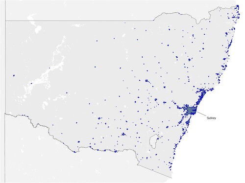
The data used for the analysis are primarily from the New South Wales Valuer General (NSWVG) and the Australian Bureau of Statistics (ABS). They are aggregated to two sets of regions: towns or cities for the whole state and neighbourhoods in the Sydney metropolitan area. The towns and cities are represented by the 2016 ABS definitions of Urban Centres and Localities (UCLs), which capture the contiguous developed area or commuting footprint around each town or city core. The UCLs are illustrated in the map in Figure 1. The neighbourhoods in Sydney are represented by the 2016 ABS definitions of Statistical Areas Level 1 (SA1s) for the whole of the Sydney UCL.

Figure 1. Map of New South Wales with the sample UCLs.

Map showing New South Wales and the sample UCLs, which dot the state but are concentrated around the large Sydney metropolitan area and the coast.

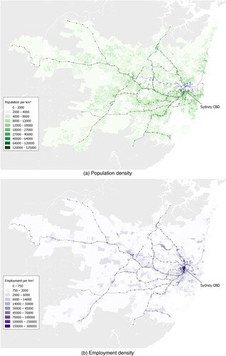
The maps in Figure 2 show the Sydney UCL in detail. The maps are shaded for the levels of population and employment density in 2016, based on statistics from the Census of that year. The maps also show the routes of passenger railways and light-rail lines and the locations of railway stations, light-rail stops and ferry wharves.

Figure 2. Maps showing SA1-level population and employment density in 2016 in the Sydney UCL.

Maps of the Sydney metropolitan area showing the rail and ferry routes, which are focused on the CBD, and shaded for the densities of population and employment, which are stronger around the CBD.

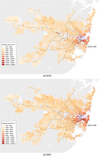
The residential property values are from the ‘bulk property sales’ data published by the NSWVG. That dataset includes all properties transacted in New South Wales and details the purchase price, location, contract and settlement dates, land area, and zoning code. However, it does not include any further details on the types or characteristics of the properties transacted. To reflect the general market values of residential properties by neighbourhood and year, while minimising the bias from differences in the types of properties transacted, the property values used in the analysis are the median price per square metre of ‘residential’ properties transacted in each UCL or SA1 and in each calendar year from 2014 to 2022. As the data on land area do not separate individual strata units, any transactions for individual strata units are excluded. The data are further limited to properties with a land area of between 100 and 4000 square metres and with a transaction price of $10,000 or more, which excludes many parking spots, farms, and other properties incorrectly coded as ‘residential’ in the NSWVG data. Properties with sale prices of less than $100 or more than $100,000 per square metre are excluded, which removes some apparently erroneous outliers. The median residential property prices by SA1 in the Sydney UCL in 2019 and 2021 are shown in the maps in Figure 3.

Figure 3. Maps showing SA1-level median residential property prices in the Sydney UCL in 2019 and 2021, both in 2019 dollars.

Maps of the Sydney metropolitan area shaded for the residential property price levels by SA1 in 2019 and 2021, which are generally higher near the CBD and beach but no patterns of differences between 2019 and 2021 are obvious.

The main factors for property prices are the populations and distances from Sydney and the coast for the UCLs and the travel times to the CBD, nearest beach and nearest point on Sydney Harbour for the SA1s in the Sydney area. The populations of the UCLs are from the 2016 Census and the distances to Sydney and the coast are crow distances based on the central post office or (if none exists) the most prominent cluster of economic activity of each UCL. The road travel times were looked up using the Open Source Routing Machine (OSRM). The travel times by train, light rail or ferry are the minimum-time trips based on their timetables from Transport for NSW, with access to train stations, light-rail stops and ferry wharves taken from the OSRM and doubled to reflect waiting times and the potential that access would involve walking or bus trips. Plots presented in Appendix B show the relationships between property prices and the populations, distances and travel times by UCL or SA1 in 2019 and 2021.

The analysis also uses neighbourhood-level statistics on geography, climate, demography and crime as controls. The mean land elevations of the UCLs and SA1s are from Geoscience Australia. The climate variables are the mean January and July temperatures and annual rainfall from the Bureau of Meteorology. The demographic variables are the rate of population growth between 2011 and 2016 and the mean age and proportions of adults who have obtained year 10 or university education in 2016 from the ABS. The crime statistics are the rates of breaking and entering, robbery and non-domestic assault in 2019–20 from the New South Wales Bureau of Crime Statistics and Research.

The variables in the UCL-level dataset are summarised in Table 1. The variables in the Sydney SA1-level dataset are summarised in Table 2. Each table has the time-invariant variables in the upper part and the property variables that are defined by region and year in the lower part.

Table 1. Summary statistics for the main variables in the UCL-level dataset.

	Mean	Std. dev.	Minimum	Maximum
Data by UCL (532 observations):
Population in 2016	12,998	188,602	107	4,321,412
Distance to Sydney CBD (km)	311.1	187.8	0.0	933.4
Distance to coast (km)	107.2	132.2	0.1	610.5
Mean land elevation (m)	226.2	286.0	2.4	1,846.8
Mean January temperature (°C)	29.0	2.8	21.9	37.1
Mean July temperature (°C)	16.0	2.7	5.6	20.6
Mean annual rainfall (mm)	934.6	358.2	244.5	1884.8
Population in 2016 / population in 2011	1.052	0.068	0.915	1.492
Mean age	42.4	3.8	33.6	54.7
Proportion of adults with year-10 education	0.831	0.035	0.759	0.914
Proportion of adults with university degree	0.151	0.056	0.060	0.324
Rate of breaking and entering (per 100 k residents)	108.8	99.4	73.2	832.2
Rate of robbery (per 100 k residents)	6.5	0.5	6.4	12.5
Rate of non-domestic assault (per 100 k residents)	138.7	31.6	131.7	709.4
Data by UCL and year (5922 observations):
Number of non-strata residential property transactions	170.1	1826.5	1	50,665
Median size of property (m^2)	1004.3	522.8	200	4000
Median purchase price (AUD)	472,761.5	324,518.2	33,000	5,000,000
Median purchase price per m^2 (AUD)	550.4	468.2	100.1	8750.0

Table 2. Summary statistics for the main variables in the Sydney SA1-level dataset.

	Mean	Std. dev.	Minimum	Maximum
Data by SA1 (9870 observations):
Travel time by road to Sydney CBD (minutes)	28.1	13.3	0.4	77.3
Travel time by road to beach (minutes)	30.3	17.3	0.2	94.8
Travel time by road to Sydney Harbour (minutes)	24.3	13.8	0.1	77.2
Travel time by rail or ferry to Sydney CBD (minutes)	47.6	21.0	0.7	119.7
Mean land elevation (m)	55.9	46.9	0.6	460.6
Mean January temperature (°C)	27.8	1.2	25.2	30.5
Mean July temperature (°C)	17.2	0.3	15.8	17.8
Mean annual rainfall (mm)	965.1	165.3	301.9	1212.0
Population in 2016 / population in 2011	1.106	0.164	0.300	11.600
Mean age	37.3	2.7	31.0	51.9
Proportion of adults with year-10 education	0.875	0.051	0.667	1.000
Proportion of adults with university degree	0.322	0.140	0.000	0.623
Rate of breaking and entering (per 100 k residents)	252.8	276.2	73.2	832.2
Rate of robbery (per 100 k residents)	11.9	15.9	6.4	67.4
Rate of non-domestic assault (per 100 k residents)	235.1	249.0	131.7	1029.3
Data by SA1 and year (86,572 observations):
Number of non-strata residential property transactions	5.1	8.8	1	867
Median size of property (m^2)	590.4	263.4	100	4000
Median purchase price (AUD)	1,401,786.4	1,410,314.7	36,050	150,000,000
Median purchase price per m^2 (AUD)	2992.6	3380.3	201.3	83,891.8

4. RESULTS

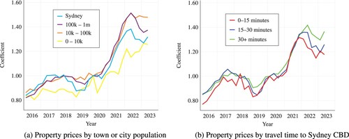
An initial observation of the data suggests that residential property prices generally rose in relative terms during the pandemic in medium-sized cities and in more distant suburbs of Sydney. Figure 4 shows indices of median residential property prices by quarter, normalised to the first quarter of 2020, for groups of UCLs in New South Wales and suburbs in Sydney. The plot on the left shows that prices have had the highest growth after early 2020 in UCLs with populations between 10,000 and 1 million. The plot on the right shows that prices have grown the most in Sydney suburbs more than 30 minutes from the CBD and the least in suburbs within 15 minutes of the CBD. Furthermore, there is no obvious long-term trend in either plot before the pandemic began.

Figure 4. Quarterly median property prices per square metre from 2016 to June 2023, normalised to the first quarter of 2020. The plots compare towns or cities in New South Wales by population and neighbourhoods in the Sydney metropolitan area by road travel time to the CBD.

Plots of quarterly property prices by town and city population and by distance of neighbourhood in the Sydney metropolitan area, normalised to the first quarter of 2020. No consistent patterns are evident before Q1 2020, but after that the prices grow in relative terms in medium-sized cities and in less central parts of Sydney.

The remainder of the analysis is arranged as per the two panels of Figure 4, with separate treatment of all UCLs in the state and the SA1s in the Sydney area.

4.1. Towns and cities in New South Wales

This section presents the analysis of the premiums in residential property prices at the UCL level on proximity to economic activity and amenities. Table 3 presents the results of the estimation of (1) at the UCL level, with the three types of access – the (log) UCL population in 2016, distance to Sydney, and distance to the coast – in separate regressions for each year. The coefficients represent the premiums on the local population and proximity to the Sydney area and the coast and the estimation is run separately for each year from 2014 to 2022, so the changes in the property-price premiums can be inferred by comparing the coefficients across columns. All of the controls described in Section 3 are used in the estimation, though their coefficients are not displayed as their values are not relevant to the main topic of this paper. Appendix C presents a set of results that demonstrate the roles of the controls in the estimation.

Table 3. OLS estimation results for the UCL-level relationships between (log) residential property prices by year and the (log) UCL population, distance to Sydney, and distance to the coast, with the populations and distances in separate regressions.

Year	(1) 2014	(2) 2015	(3) 2016	(4) 2017	(5) 2018	(6) 2019	(7) 2020	(8) 2021	(9) 2022
Panel A. Estimates using UCL population in 2016
ln (population)	0.135^a (0.015)	0.150^a (0.015)	0.158^a (0.014)	0.162^a (0.015)	0.161^a (0.014)	0.147^a (0.014)	0.148^a (0.015)	0.160^a (0.016)	0.153^a (0.017)
R^2	0.60	0.62	0.64	0.67	0.69	0.69	0.68	0.71	0.72
Panel B. Estimates using distance to Sydney CBD
ln (distance to Sydney CBD)	−0.163^a (0.045)	−0.208^a (0.052)	−0.204^a (0.057)	−0.217^a (0.057)	−0.212^a (0.056)	−0.167^a (0.046)	−0.167^a (0.047)	−0.183^a (0.049)	−0.181^a (0.052)
R^2	0.58	0.61	0.62	0.65	0.67	0.66	0.65	0.69	0.70
Panel C. Estimates using distance to nearest coast
ln (distance to coast)	−0.099^a (0.014)	−0.089^a (0.013)	−0.110^a (0.014)	−0.121^a (0.015)	−0.145^a (0.016)	−0.150^a (0.014)	−0.166^a (0.019)	−0.171^a (0.015)	−0.197^a (0.019)
R^2	0.65	0.66	0.67	0.70	0.71	0.71	0.71	0.73	0.74
Number of observations	483	492	498	497	493	490	497	499	506

Note: Robust standard errors in parentheses; a, b, c denote significance at 1%, 5%, 10%; the dependent variable in each regression is the (log) median sale price per square metre for residential properties in the UCL in the given year; all regressions include the full range of controls for geography, climate, demography and crime, the coefficients on which are not displayed.

Figure 5 plots the coefficients from Table 3, to facilitate comparison of them over time. The plots display p-values from Wald tests of the differences between the coefficients for intervals of one or two years, if those p-values are less than 10%.

Figure 5. Coefficients on (log) UCL population and distances to Sydney and the coast, from separate regressions.

The coefficients on proximity in the property-prices of towns and cities, estimated from separate regressions, show no clear pattern or effect of the pandemic.

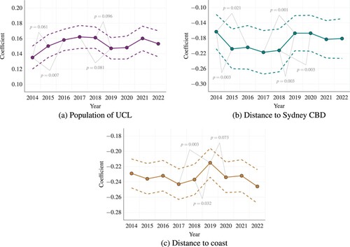
The results in Table 3 and Figure 5 do not show any discernible trend in the property-price premiums related to the timing of the pandemic. For the UCL population and distance to Sydney, some of the changes in the coefficients are significant, but none of those are driven by differences that occur after 2019 – there is a significant difference between the coefficients on log distance to Sydney in 2018 and 2020 but the level of that coefficient did not change between 2019 and 2020. There is a significant shift downwards in the coefficient on log distance to the coast between 2019 and 2020, but that is a return to near the level of the coefficients for 2018 and earlier years, so the 2019 value may simply be an outlier.

To address the limitation of some types of proximity potentially being proxies for others, Table 4 and Figure 6 present a similar analysis to Table 3 and Figure 5 but with all three types of proximity in the same regression for each year.

Figure 6. Coefficients on (log) UCL population and distances to Sydney and the coast, from the same regression for each year.

The coefficients on proximity in the property-prices of towns and cities, estimated from the same regressions, show no clear pattern or effect of the pandemic.

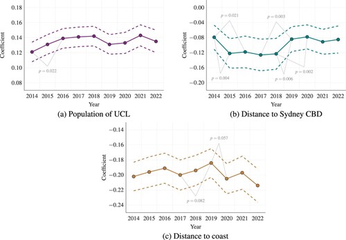
Table 4. OLS estimation results for the UCL-level relationships between (log) residential property prices by year and the (log) UCL population, distance to Sydney, and distance to the coast, with the populations and distances in the same regression for each year.

	(1)	(2)	(3)	(4)	(5)	(6)	(7)	(8)	(9)
Year	2014	2015	2016	2017	2018	2019	2020	2021	2022
ln (population)	0.121^a	0.131^a	0.139^a	0.141^a	0.142^a	0.131^a	0.133^a	0.143^a	0.135^a
	(0.013)	(0.013)	(0.013)	(0.013)	(0.013)	(0.013)	(0.014)	(0.014)	(0.015)
ln (distance to Sydney CBD)	−0.079^b	−0.122^a	−0.118^a	−0.118^a	−0.126^a	−0.084^b	−0.078^b	−0.091^a	−0.085^b
	(0.032)	(0.039)	(0.042)	(0.042)	(0.041)	(0.033)	(0.032)	(0.033)	(0.036)
ln (distance to coast)	−0.202^a	−0.196^a	−0.191^a	−0.200^a	−0.194^a	−0.184^a	−0.205^a	−0.197^a	−0.214^a
	(0.019)	(0.020)	(0.020)	(0.020)	(0.020)	(0.019)	(0.020)	(0.022)	(0.022)
R^2	0.71	0.74	0.74	0.77	0.78	0.76	0.76	0.78	0.79
Number of observations	483	492	498	497	493	490	497	499	506

Note: Robust standard errors in parentheses; a, b, c denote significance at 1%, 5%, 10%; the dependent variable in each regression is the (log) median sale price per square metre for residential properties in the UCL in the given year; all regressions include the full range of controls for geography, climate, demography and crime, the coefficients on which are not displayed.

The results in Table 4 and Figure 6 resemble those with the three types of proximity applied separately, but are somewhat cleaner. The standard errors on the estimated coefficients on log distance to Sydney are smaller when all three measures of proximity are used, possibly because the UCL population or distance to the coast explain a substantial amount of the variation in property prices that does not correlate well with distance to Sydney. While the trends in the coefficients appear similar, there are fewer significant changes when all three types of proximity are used in the same regression. Again no significant changes appear after 2019, except for (i) the change in the coefficient on log distance to Sydney between 2018 and 2020 that appears to be due to the change between 2018 and 2019 and (ii) the change in the coefficient on log distance to the coast between 2019 and 2020 that appears to be a return to the level of 2018 and earlier.

A limitation of the analysis presented above is that, although it measures how the premiums on access have changed, it does so in a (log) linear fashion. The overall trends in the property-price data in the first panel of Figure 4 suggest that the changes may in fact have been non-linear, as there was a relative price increase in UCLs of intermediate size. To address the potential non-linearity while accounting for the effects of the controls, Table 5 compares coefficients from the estimation of (1) with the second moment of log UCL population and the log distances. To keep the analysis succinct, only the years 2019 and 2021 are compared and the p-values from Wald tests of the differences between them are displayed in the table.

Table 5. OLS estimation results for the UCL-level relationships between (log) residential property prices in 2019 and 2021 and the first two moments of (log) UCL population, distance to Sydney and distance to the coast.

	(1)	(2)	(3)	(4)	(5)	(6)	(7)	(8)
Year	2019	2021	2019	2021	2019	2021	2019	2021
ln (population)	0.228^a	0.286^a					0.350^a	0.450^a
	(0.079)	(0.091)					(0.089)	(0.093)
	[p = 0.199]						[p = 0.078]
ln (population)^2	-0.005	-0.008					−0.014^a	−0.020^a
	(0.005c)	(0.005)					(0.005)	(0.006)
	[p = 0.255]						[p = 0.088]
ln (distance to Sydney CBD)			−0.040^c	−0.052^b			−0.069^b	−0.104^a
			(0.021)	(0.025)			(0.027)	(0.028)
			[p = 0.096]				[p = 0.016]
ln (distance to Sydney CBD)^2			−0.020^a	−0.020^a			−0.006	−0.003
			(0.003)	(0.004)			(0.004)	(0.004)
			[p = 0.833]				[p = 0.237]
ln (distance to coast)					−0.147^a	−0.164^a	−0.168^a	−0.186^a
					(0.027)	(0.030)	(0.026)	(0.030)
					[p = 0.285]		[p = 0.272]
ln (distance to coast)^2					−0.031^a	−0.030^a	−0.004	−0.002
					(0.008)	(0.009)	(0.009)	(0.010)
					[p = 0.898]		[p = 0.676]
R^2	0.69	0.71	0.67	0.69	0.72	0.73	0.77	0.79
Number of observations	490	499	490	499	490	499	490	499

Note: Robust standard errors in parentheses and p-values or differences between coefficients in square brackets; a, b, c denote significance at 1%, 5%, 10%; the dependent variable in each regression is the (log) median sale price per square metre for residential properties in the UCL in the given year; all regressions include the full range of controls for geography, climate, demography and crime, the coefficients on which are not displayed.

The results in Table 5 support the idea that the premium increased in towns and cities of intermediate size. In the regressions that use all three types of proximity, the coefficients on the two moments of log UCL population increase significantly in magnitude, if only at the 10% level. The increase in the magnitude of the (negative) second moment means that property prices increase in relative terms in UCLs in the middle of the population distribution. The other coefficients that change significantly are those on the first moment of the log distance to Sydney, which increase in magnitude, though it is unclear how this should be interpreted given the lack of any clear effect in the linear estimation above.

4.2. Neighbourhoods in Sydney

We now turn to a detailed analysis of the SA1s in the Sydney metropolitan area. Table 6 presents the results of the estimation of Equation (1) with each of the log travel-time variables used as $V_r$ in a separate set of regressions. The coefficients on the log travel times represent the slopes of the respective property-price gradients and again the estimation is run separately for each year from 2014 to 2022. As with the UCL-level estimation, all of the SA1-level controls are used in the estimation and their coefficients are not displayed, though results that demonstrate how the controls affect the estimation are presented in Appendix C. Figure 7 plots the coefficients from Table 6, with the p-values from Wald tests of the differences over intervals of one or two years displayed if less than 10%.

Figure 7. Coefficients on (log) travel times by road to the Sydney CBD, the beach and Sydney Harbour and by rail or ferry to the CBD, from separate regressions.

The coefficients on proximity in the property-prices of Sydney SA1s, estimated from separate regressions, show (i) decreased premiums on proximity to the CBD by road or rail and ferry during the pandemic and (ii) a steady increase in the premium on proximity to the beach since 2015 that continues through the pandemic with no obvious change.

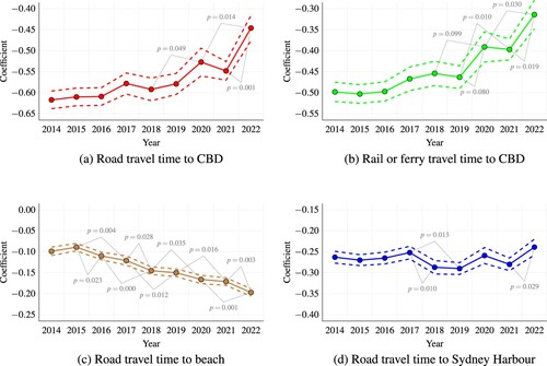
Table 6. OLS estimation results for the SA1-level relationships between (log) residential property prices by year in the Sydney metropolitan area and each type of (log) travel time, with the travel times in separate regressions.

Year	(1) 2014	(2) 2015	(3) 2016	(4) 2017	(5) 2018	(6) 2019	(7) 2020	(8) 2021	(9) 2022
Panel A. Estimates using travel time by road to Sydney CBD
ln (travel time by road to Sydney CBD)	−0.617^a (0.021)	−0.610^a (0.021)	−0.609^a (0.021)	−0.578^a (0.025)	−0.592^a (0.027)	−0.579^a (0.025)	−0.527^a (0.033)	−0.548^a (0.022)	−0.446^a (0.030)
R^2	0.78	0.78	0.78	0.78	0.77	0.77	0.75	0.79	0.76
Panel B. Estimates using travel time by rail or ferry to Sydney CBD
ln (travel time by rail / ferry to Sydney CBD)	−0.498^a (0.023)	−0.503^a (0.022)	−0.497^a (0.023)	−0.467^a (0.028)	−0.454^a (0.029)	−0.463^a (0.027)	−0.391^a (0.036)	−0.397^a (0.025)	−0.314^a (0.034)
R^2	0.77	0.77	0.77	0.77	0.75	0.75	0.74	0.78	0.76
Panel C. Estimates using travel time by road to nearest beach
ln (travel time by road to beach)	−0.099^a (0.010)	−0.089^a (0.009)	−0.110^a (0.009)	−0.121^a (0.011)	−0.145^a (0.009)	−0.150^a (0.009)	−0.166^a (0.010)	−0.171^a (0.009)	−0.197^a (0.009)
R^2	0.76	0.76	0.76	0.76	0.75	0.75	0.74	0.78	0.77
Panel D. Estimates using travel time by road to Sydney Harbour
ln (travel time by road to Sydney Harbour)	−0.263^a (0.014)	−0.270^a (0.013)	−0.265^a (0.014)	−0.252^a (0.015)	−0.287^a (0.016)	−0.290^a (0.014)	−0.259^a (0.019)	−0.280^a (0.015)	−0.239^a (0.019)
R^2	0.77	0.78	0.77	0.78	0.76	0.76	0.75	0.79	0.77
Number of observations	8041	7997	7841	7840	7570	7687	7763	8108	7988

Note: robust standard errors in parentheses; a, b, c denote significance at 1%, 5%, 10%; the dependent variable in each regression is the (log) median sale price per square metre for residential properties in the SA1 in the given year; all regressions include the full range of controls for geography, climate, demography, and crime, the coefficients on which are not displayed.

Observing Table 6 and Figure 7, the premiums on log travel time to the Sydney CBD, whether measured as the travel time by road or by rail or ferry, appear to have eroded since 2019. The Wald tests of the differences between the coefficients confirm this. The coefficients on log travel time to the beach have increased in magnitude over time, significantly so for most intervals, but with no obvious relationship to the timing of the pandemic. The coefficients on log travel time to Sydney Harbour have no obvious trend. Note that relatively many of the changes for the travel times to the beach are significant though the sizes of their differences are smaller than for the other variables, as the former have relatively small standard errors. This is because the travel times to the beach explain property prices more consistently than the travel times to the CBD or the Harbour.

Table 7 and Figure 8 present the results of the analysis that uses all four types of travel-time variables in the same regression for each year. This analysis should better reflect the combined effects of the four types of proximity.

Figure 8. Coefficients on (log) travel times by road to the Sydney CBD, the beach and Sydney Harbour and by rail or ferry to the CBD, from the same regression for each year.

The coefficients on proximity in the property-prices of Sydney SA1s, estimated from the same regressions, show (i) a decreased premium on proximity to the CBD by rail or ferry in 2020 and 2021, (ii) a decreased premium on proximity to the CBD by road in 2022, and (iii) a steady increase in the premium on proximity to the beach since 2015 that continues through the pandemic with no obvious change.

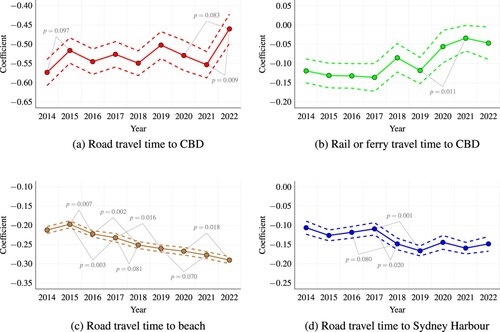
Table 7. OLS estimation results for the SA1-level relationships between (log) residential property prices by year in the Sydney metropolitan area and each type of (log) travel time, with all four types of travel time in the same regression for each year.

Year	(1) 2014	(2) 2015	(3) 2016	(4) 2017	(5) 2018	(6) 2019	(7) 2020	(8) 2021	(9) 2022
ln (travel time by road to Sydney CBD)	−0.573^a	−0.516^a	−0.545^a	−0.526^a	−0.549^a	−0.502^a	−0.529^a	−0.553^a	−0.460^a
	(0.034)	(0.033)	(0.033)	(0.033)	(0.032)	(0.035)	(0.039)	(0.034)	(0.038)
ln (travel time by rail / ferry to Sydney CBD)	−0.119^a	−0.131^a	−0.132^a	−0.136^a	−0.085^b	−0.118^a	−0.056	−0.034	−0.047
	(0.031)	(0.032)	(0.032)	(0.036)	(0.037)	(0.034)	(0.042)	(0.033)	(0.042)
ln (travel time by road to beach)	−0.212^a	−0.197^a	−0.222^a	−0.232^a	−0.251^a	−0.260^a	−0.267^a	−0.277^a	−0.290^a
	(0.009)	(0.009)	(0.008)	(0.011)	(0.009)	(0.009)	(0.010)	(0.009)	(0.009)
ln (travel time by road to Sydney) Harbour)	−0.106^a	−0.126^a	−0.118^a	−0.109^a	−0.148^a	−0.166^a	−0.144^a	−0.159^a	−0.148^a
	(0.017)	(0.014)	(0.015)	(0.016)	(0.015)	(0.013)	(0.018)	(0.015)	(0.019)
R^2	0.80	0.80	0.80	0.81	0.79	0.80	0.78	0.83	0.80
Number of observations	8041	7997	7841	7840	7570	7687	7763	8108	7988

Note: Robust standard errors in parentheses; a, b, c denote significance at 1%, 5%, 10%; the dependent variable in each regression is the (log) median sale price per square metre for residential properties in the SA1 in the given year; all regressions include the full range of controls for geography, climate, demography and crime, the coefficients on which are not displayed.

The results in Table 7 and Figure 8 show a distinction in how the two types of proximity to the CBD have been valued since 2019. The coefficients on the log travel time by road to the CBD do not significantly change between 2019 and 2021, then decrease in magnitude significantly in 2022. The coefficients on the log travel time by rail or ferry increase in raw terms between 2019 and 2021 (they are positive for most years, apparently due to the interaction with the road travel times). These results imply that the premium on access to the CBD by road remained fairly constant until 2021, then decreased in 2022, while the premium on access by public transport decreased substantially between 2019 and 2021 but then did not change between 2021 and 2022.

The results for proximity to the beach and to Sydney Harbour in Table 7 and Figure 8 are broadly consistent with the estimates with each type of log travel time in a separate regression. That is, the coefficients on log travel time by road to the beach have been decreasing on a constant trend since 2015, whereas the coefficients on log travel time by road to Sydney Harbour have no obvious trend. Moreover, there is no obvious effect of the pandemic.

Appendix D repeats the analysis in Table 7 and Figure 8 using quarterly data from 2016 to the second quarter of 2023. The quarterly results have more variation but have no obvious seasonality and are broadly consistent with the annual results. Furthermore, the coefficients on log travel time in the estimation for 2022 have persisted into the first two quarters of 2023.

5. CONCLUSION

The COVID-19 pandemic has caused widespread changes to societies around the world, some of which may end up being permanent. These include changes to how people work, travel and use amenities, which have implications for the values of residential land. This paper tests how the values of proximity to employment and amenities in New South Wales, as reflected in the sale prices of properties, have changed since 2019. The analysis is carried out on two sets of geographical units. The first is the towns and cities in New South Wales, for which the premiums on population and the distances to Sydney and the coast are estimated. The second is the neighbourhoods in the Sydney metropolitan area, for which the premiums on travel time to the Sydney CBD, the beach and Sydney Harbour are estimated.

The analysis shows that, between 2019 and 2021, property prices grew in relative terms in towns and cities of intermediate size. For the Sydney area, the findings are that: (1) the premium on proximity to the CBD has decreased since 2019; (2) the decreased premium on proximity to the CBD was initially explained by a lower premium on proximity by public transport, but then between 2021 and 2022 the premium on proximity by car also decreased; (3) the premium on proximity to the beach has increased since 2019, though this is consistent with an existing trend and (4) there is no obvious effect of the pandemic on the premium on proximity to Sydney Harbour.

The finding that prices increased in relative terms in medium-sized towns and cities could be explained by a shift in demand from the Sydney area to smaller cities that are large enough to have substantial services and amenities, as found for the US by Liu and Su (2021). This would also be consistent with a partial shift to remote work, which allows people to live away from the expensive Sydney area even if they are employed there.

The first result for Sydney, that the proximity to the CBD appears to have declined in value, fits with intuition about the effects of policies adopted there, as in many other places, to address COVID-19. Those policies forced working-from-home where possible, which affected office workers in particular. Due to the large amount of office space in the CBD, this has greatly reduced the overall benefits for Sydney residents of living in proximity to the CBD. The CBD also has high densities of shopping, restaurants, museums, entertainment and other amenities, much of which was limited or closed due to COVID-19 policies. Thus it makes sense that the premiums on proximity to these amenities would have decreased.

The second result for Sydney corresponds to changes in the limitation of different types of transport and thus their utilisation since 2019. In the peak years of the pandemic – 2020 and 2021 – travel activity was low but public transport use was especially low, due to an apparent combination of fear of infection, the hassles of digital check-ins and mask mandates discouraging passengers, and limited services.⁵ During this time, the premium on proximity to the CBD via public transport decreased. As pandemic restrictions were removed between late 2021 and early 2022, passengers returned to public transport but a degree of working-from-home remained. This corresponded with a continued low premium on proximity to the CBD but a shift away from the premium on access by road.

The third and fourth results for Sydney reflect there being no measurable effect of the pandemic on the relative value of proximity to two natural amenities: the beach and Sydney Harbour. The premium on proximity to the beach has been steadily increasing since 2015 and the differences in gradient have been significant for many intervals of one or two years, but there is no obvious difference after 2019 relative to the previous trend. There has been a general slight increase in the premiums on proximity to the Harbour over the period from 2014 to 2022, but the differences are only significant for a few intervals and, as with the beach, there is no obvious change relative to the existing trend after 2019.

Even if the recent circumstances have changed factors for the current value of property, it is not obvious that these changes would be reflected in house prices. How much one is willing to pay for a house should reflect a discounted series of valuations for many periods into the future. Thus a temporary change in circumstances, especially if it is perceived to have ended, should not make a substantial difference to house prices. The fact that house prices in Sydney appear to have changed, even after the pandemic policies have ended, suggests that the changes to current values are substantial and that there is at least a perception that the societal changes caused by the pandemic will linger for a substantial period of time. An example would be the permanent shift to working-from-home, whether driven by workers’ preferences or cost savings for firms, as reflected in the stated openness to work from home even after the pandemic, identified by Beck et al. (2020). Note that the pandemic and related policies were not anticipated to any significant degree, so we can be confident that it would not have factored into property values up to 2019.

The work presented in this paper has a number of limitations. Firstly, the data on property transactions from the NSWVG do not include details on the type of property, such as structure size or age, so it is difficult to fully exclude the possibility of the trends in property-price gradients simply being artefacts of changes in property types. Secondly, the data are for a single state, whereas the US studies cited above use data on many jurisdictions, though it is beneficial to have evidence of the effects of a phenomenon from other places. Thirdly, as the proximate effects of the COVID-19 situation are still recent, it is possible that different trends will become apparent in the fullness of time. All of these limitations represent potential avenues for future research, which should eventually generate a clearer picture of the effects of the COVID-19 pandemic on house prices.

ACKNOWLEDGEMENTS

The author thanks Sasan Bakhtiari, James Lennox and seminar participants at Deakin University, Victoria University, the 2022 Australian Conference of Economists and the 2022 Australian Workshop on Public Finance for helpful comments and suggestions. All remaining errors are due to the author.

DATA AVAILABILITY STATEMENT

The data used in this research were assembled from several public sources, as detailed in the Data section above, and are free to download with no permission required. The primary sources were the New South Wales Valuer General and the Australian Bureau of Statistics. Other data were from the Open Source Routing Machine, Transport for NSW, Geoscience Australia, the Bureau of Meteorology, and the New South Wales Bureau of Crime Statistics and Research.

DISCLOSURE STATEMENT

No potential conflict of interest was reported by the author.

Notes

1 The classic model of Roback (1982) is commonly used to study the relationships between jobs, amenities and land prices at the level of cities or regions. The gradients of residential property prices with distance from the city centre are represented by the classic monocentric city paradigm of Alonso (1964), Mills (1967) and Muth (1969), even if Ahlfeldt (2011) showed that, at least in Berlin, they are explained substantially better by a model that generalises the proximity to all employment locations and accounts for travel accessibility by mode. The gradients in property prices within cities by distance from amenities such as parks, lakes, beaches, restaurants or shopping have been demonstrated by Diamond (1980), Tyrväinen and Miettinen (2000), Cho (2001) and Kovacs and Larson (2007).

2 A broader literature has analysed the effects of COVID-19 policies, for example on mental health (Fisher et al., 2020; Marques de Miranda et al., 2020; O’Connor et al., 2021; Robinson et al., 2022; Altindag et al., 2022), substance abuse (Avena et al., 2021; Root et al., 2021) and student achievement (Gore et al., 2021; Hammerstein et al., 2021).

3 The amenities tested are the beach and Harbour because they are easily measurable and have important variation at the neighbourhood level, whereas amenities such as restaurants, parks and schools are present in most neighbourhoods and have characteristics that are difficult to quantify.

4 There is evidence of people shifting away from public transport in 2020 in Germany (Eisenmann et al., 2021), Sweden (Jenelius & Cebecauer, 2020) and Israel (Elias & Zatmeh-Kanj, 2021). Moreover, Chen et al. (2022) found that use of public transport decreased in Taiwan even though there were no government restrictions on its use, while highway traffic actually increased.

5 Other research confirms a shift from public transport to car use during the pandemic in Germany (Eisenmann et al. (2021)), Sweden (Jenelius & Cebecauer, 2020), Israel (Elias & Zatmeh-Kanj, 2021) and Taiwan (Chen et al., 2022).

REFERENCES

- Ahlfeldt, G. (2011). If Alonso was right: Modeling accessibility and explaining the residential land gradient. Journal of Regional Science, 51(2), 318–338. https://doi.org/10.1111/j.1467-9787.2010.00694.x
- Alonso, W. (1964). Location and land use. Harvard University Press.
- Althoff, L., Eckert, F., Ganapati, S., & Walsh, C. (2022). The geography of remote work. Regional Science and Urban Economics, 93, 103770. https://doi.org/10.1016/j.regsciurbeco.2022.103770
- Altindag, O., Erten, B., & Keskin, P. (2022). Mental health costs of lockdowns: Evidence from age-specific curfews in Turkey. American Economic Journal: Applied Economics, 14(2), 320–343. https://doi.org/10.1257/app.20200811
- Avena, N. M., Simkus, J., Lewandowski, A., Gold, M. S., & Potenza, M. N. (2021). Substance use disorders and behavioral addictions during the COVID-19 pandemic and COVID-19-related restrictions. Frontiers in Psychiatry, 12, 653674. https://doi.org/10.3389/fpsyt.2021.653674
- Batalha, M., Goncalves, D., Peralta, S., & Pereira dos Santos, J. (2022). The virus that devastated tourism: The impact of Covid-19 on the housing market. Regional Science and Urban Economics, 95, 103774. https://doi.org/10.1016/j.regsciurbeco.2022.103774
- Beck, M. J., Hensher, D. A., & Wei, E. (2020). Slowly coming out of COVID-19 restrictions in Australia: Implications for working from home and commuting trips by car and public transport. Journal of Transport Geography, 88, 102846. https://doi.org/10.1016/j.jtrangeo.2020.102846
- Bendavid, E., Oh, C., Bhattacharya, J., & Ioannidis, J. P. A. (2021). Assessing mandatory stay-at-home and business closure effects on the spread of COVID-19. European Journal of Clinical Investigation, 51(4), e13484. https://doi.org/10.1111/eci.13484
- Chen, K.-P., Yang, J.-C., & Yang, T.-T. (2022). JUE insight: Demand for transportation and spatial pattern of economic activity during the pandemic. Journal of Urban Economics, 127, 103426. https://doi.org/10.1016/j.jue.2022.103426
- Cheung, K. S., Yiu, C. Y., & Xiong, C. (2021). Housing market in the time of pandemic: A price gradient analysis from the COVID-19 epicentre in China. Journal of Risk and Financial Management, 14(3), 108. https://doi.org/10.3390/jrfm14030108
- Cho, C.-J. (2001). Amenities and urban residential structure: An amenity-embedded model of residential choice. Papers in Regional Science, 80(4), 483–498. https://doi.org/10.1111/j.1435-5597.2001.tb01215.x
- de Haas, M., Faber, R., & Hamersma, M. (2020). How COVID-19 and the Dutch ‘intelligent lockdown’ change activities, work and travel behaviour: Evidence from longitudinal data in The Netherlands. Transportation Research Interdisciplinary Perspectives, 6, 100150. https://doi.org/10.1016/j.trip.2020.100150
- Diamond, D. B. (1980). The relationship between amenities and urban land prices. Land Economics, 56(1), 21–32. https://doi.org/10.2307/3145826
- D’Lima, W., Lopez, L. A., & Pradhan, A. (2022). COVID-19 and housing market effects: Evidence from U.S. Shutdown orders. Real Estate Economics, 50(2), 303–339. https://doi.org/10.1111/1540-6229.12368
- Eisenmann, C., Nobis, C., Kolarova, V., Lenz, B., & Winkler, C. (2021). Transport mode use during the COVID-19 lockdown period in Germany: The car became more important, public transport lost ground. Transport Policy, 103, 60–67. https://doi.org/10.1016/j.tranpol.2021.01.012
- Elias, W., & Zatmeh-Kanj, S. (2021). Extent to which COVID-19 will affect future use of the train in Israel. Transport Policy, 110, 215–224. https://doi.org/10.1016/j.tranpol.2021.06.008
- Fisher, J. R. W., Tran, T. D., Hammarberg, K., Sastry, J., Nguyen, H., Rowe, H., Popplestone, S., Stocker, R., Stubber, C., & Kirkman, M. (2020). Mental health of people in Australia in the first month of COVID-19 restrictions: A national survey. The Medical Journal of Australia, 213(10), 458–464. https://doi.org/10.5694/mja2.50831
- Gore, J., Fray, L., Miller, A., Harris, J., & Taggart, W. (2021). The impact of COVID-19 on student learning in New South Wales primary schools: An empirical study. The Australian Educational Researcher, 48(4), 605–637. https://doi.org/10.1007/s13384-021-00436-w
- Gupta, A., Mittal, V., Peeters, J., & Van Nieuwerburgh, S. (2022). Flattening the curve: Pandemic-induced revaluation of urban real estate. Journal of Financial Economics, 146(2), 594–636. https://doi.org/10.1016/j.jfineco.2021.10.008
- Hammerstein, S., König, C., Dreisörner, T., & Frey, A. (2021). Effects of COVID-19-related school closures on student achievement-A systematic review. Frontiers in Psychology, 12, 746289. https://doi.org/10.3389/fpsyg.2021.746289
- Jenelius, E., & Cebecauer, M. (2020). Impacts of COVID-19 on public transport ridership in Sweden: Analysis of ticket validations, sales and passenger counts. Transportation Research Interdisciplinary Perspectives, 8, 100242. https://doi.org/10.1016/j.trip.2020.100242
- Kovacs, K. F., & Larson, D. M. (2007). The influence of recreation and amenity benefits of open space on residential development patterns. Land Economics, 83(4), 475–496. https://doi.org/10.3368/le.83.4.475
- Liu, S., & Su, Y. (2021). The impact of the COVID-19 pandemic on the demand for density: Evidence from the U.S. Housing market. Economics Letters, 207, 110010. https://doi.org/10.1016/j.econlet.2021.110010
- Marques de Miranda, D., da Silva Athanasio, B., Sena Oliveira, A. C., & Simoes-e-Silva, A. C. (2020). How is COVID-19 pandemic impacting mental health of children and adolescents? International Journal of Disaster Risk Reduction, 51, 101845. https://doi.org/10.1016/j.ijdrr.2020.101845
- Mills, E. S. (1967). An aggregative model of resource allocation in a metropolitan area. The American Economic Review, 57(2), 197–210. http://www.jstor.org/stable/1821621
- Muth, R. F. (1969). Cities and housing: The spatial pattern of urban residential land use. University of Chicago Press.
- O’Connor, R. C., Wetherall, K., Cleare, S., McClelland, H., Melson, A. J., Niedzwiedz, C. L., O’Carroll, R. E., O’Connor, D. B., Platt, S., Scowcroft, E., Watson, B., Zortea, T., Ferguson, E., & Robb, K. A. (2021). Mental health and well-being during the COVID-19 pandemic: Longitudinal analyses of adults in the UK COVID-19 mental health & wellbeing study. The British Journal of Psychiatry, 218(6), 326–333. https://doi.org/10.1192/bjp.2020.212
- Ramani, A., & Bloom, N. (2021). The donut effect of Covid-19 shapes real estate. Stanford Institute for Economic Policy Research (SIEPR) Policy Brief.
- Roback, J. (1982). Wages, rents, and the quality of life. Journal of Political Economy, 90(6), 1257–1278. https://doi.org/10.1086/261120
- Robinson, E., Sutin, A. R., Daly, M., & Jones, A. (2022). A systematic review and meta-analysis of longitudinal cohort studies comparing mental health before versus during the COVID-19 pandemic in 2020. Journal of Affective Disorders, 296, 567–576. https://doi.org/10.1016/j.jad.2021.09.098
- Root, E. D., Slavova, S., LaRochelle, M., Feaster, D. J., Villani, J., Defiore-Hyrmer, J., El-Bassel, N., Ergas, R., Gelberg, K., Jackson, R., Manchester, K., Parikh, M., Rock, P., & Walsh, S. L. (2021). The impact of the national stay-at-home order on emergency department visits for suspected opioid overdose during the first wave of the COVID-19 pandemic. Drug and Alcohol Dependence, 228, 108977. https://doi.org/10.1016/j.drugalcdep.2021.108977
- Rosenthal, S. S., Strange, W. C., & Urrego, J. A. (2022). JUE insight: Are city centers losing their appeal? Commercial real estate, urban spatial structure, and COVID-19. Journal of Urban Economics, 127, 103381. https://doi.org/10.1016/j.jue.2021.103381
- Shamshiripour, A., Rahimi, E., Shabanpour, R., & Mohammadian, A. K. (2020). How is COVID-19 reshaping activity-travel behavior? Evidence from a comprehensive survey in Chicago. Transportation Research Interdisciplinary Perspectives, 7, 100216. https://doi.org/10.1016/j.trip.2020.100216
- Spiegel, M., & Tookes, H. (2021). Business restrictions and COVID-19 fatalities. The Review of Financial Studies, 34(11), 5266–5308. https://doi.org/10.1093/rfs/hhab069
- Tyrväinen, L., & Miettinen, A. (2000). Property prices and urban forest amenities. Journal of Environmental Economics and Management, 39(2), 205–223. https://doi.org/10.1006/jeem.1999.1097