Novel predictive model of cell survival/death related effects of Extracellular Signal-Regulated kinase protein

Abstract

Computational modelling is a technique for modelling and solving real-world problems by utilising computing to provide solutions. This paper presents a novel predictive model of cell survival/death-related effects of Extracellular Signal-Regulated Kinase Protein. The computational model was designed using Neural Networks and fuzzy system. Three hundred ERK samples were examined using ten different concentrations of three input proteins: EGF, TNF, and insulin. Based on the different concentrations of input proteins and different samples of ERK protein, adjustment Anderson darling (AD) statistics for multiple distribution functions were computed considering different test such as visual test, Pearson correlation coefficient, and uniformity tests. The results reveal that utilising different concentrations and samples, values such as 7.55 AD and 18.4 AD were obtained using the Weibull distribution function for 0 ng/ml of TNF, 100 ng/ml of EGF, and 0 ng/mL of insulin concentrations. The model was validated by predicting the various ERK protein values that fall within the observed range. The proposed model agrees with the deterministic model, which was developed using difference equations.

Keywords:

• ERK
• Anderson Darling
• concentration
• samples
• uniformity tests
• computational model

Introduction

System biology is the study of the properties of complex biological systems that develop from the interactions of several proteins. Systems biology aims to expand organisms' behavior by utilizing scientific and technological knowledge so they can carry out new tasks. Deoxyribonucleic acid (DNA), ribonucleic acid (RNA), proteins, and metabolites (including carbohydrates, lipids, amino acids, and nucleotides) from the newly constructed behaviour’s bottom-up hierarchy are a few examples of biological systems. Biological systems have recently been compared to electronic systems, which contain a bottom-up layer consisting of a physical layer, a device layer, and a module layer [1]. Transistors, capacitors, and resistors form the physical layer, while all the computations performed in the computer by the electrical circuits form the device layer, and components like the integrated circuits form the module layer [2,3].

Engineering problems require mathematical solutions. Some problems are difficult to solve, while others necessitate precise answers that are not determinable [4]. Numerical methods and computational techniques employ computers to solve problems that are either iterative, repeating, or sequential in nature, and are frequently intractable or theoretically difficult to grasp [5]. They are powerful problem-solving tools capable of dealing with enormous quantities of equations, complex geometries, and non-linearities. Computational methods simplify complex mathematics by reducing them to fundamental arithmetic processes. Among the many applications of computer modelling is the determination of cell survival/death [6]. Computers are used in computational modelling to investigate and simulate the behaviour of complex systems in computer science, physics, and mathematics. This modelling is also an important component of big data analytics. To determine the major metabolic changes associated with cell division, signal processing approaches used for cell survival/death analysis employ a variety of computational methodologies [7]. Extracellular signals such as cytokines, growth factors, and hormones are mediated by receptors that aid in the transduction of intracellular cues [8]. Tumour necrosis factor- (TNF-) functions as a cue for programmed cell death [9], whereas epidermal growth factor (EGF) [10,11] and insulin [12,13] function as survival cues. There are different types of proteins that help in the computer engineering hierarchy. In this paper, the Extracellular Signal-Regulated Kinase (ERK) protein that forms one of the pathways of Mitogenic (MAPK) proteins [14] is investigated. MAPKs are threonine/serine protein kinases that are activated by MAP/ERK kinases (MEKs), which activates MEK kinase (MEKK). This pathway promotes cell survival by increasing transcription cell proliferation, Bcl2 family members, and inhibitors of cell death proteins (IAPs). The ERK MAP kinase cascade is one of the central pathways in growth factor signal transductions. ERK 1/2 are members of the MAPK superfamily that mediate apoptosis or cell proliferation. The RAS-Raf-MEK-ERK signalling cascade, which controls cell proliferation, has received a lot of attention in recent times. Because U0126 inhibits ERK1/2, which results in decreased branching, morphogenesis, increased mesenchymal apoptosis, and decreased epithetical proliferation in foetal lung explants, the ERK1/2 activation appears to be responsible for proper foetal lung development. ERK2 and MEK1 are more important than than ERK1 and MEK2 for embryonic development. ERK2 and MEK1 deficient mice develop a faulty placenta, whereas ERK1 or MEK2 deficient mice are viable, normal in size, and fertile. Defects in AKT signalling have been identified as the root cause of a wide range of human diseases, elucidating the downstream targets and functions that are critical to comprehend. Because the ability to knockout, knockdown, or pharmacologically inhibit specific AKT isoforms and related AGC kinases has greatly improved, previously identified substrates should be examined more rigorously. Cancer, insulin resistance, diabetes, cardiovascular disease, and autoimmune diseases are all caused by improper regulation of the AKT pathways/networks. It is regulated by growth signals/factors such as insulin. By increasing anabolism and decreasing catabolism, the AKT pathway promotes glucose uptake and utilisation, synthesis of glycogen, fatty acid, protein, and cell survival/proliferation. It is crucial for health practitioners and the academic community to develop an efficient model that will effectively regulate the signalling of the AKT pathways/networks. In this paper, the authors have worked on HT carcinoma cells.

The experimental data of the carcinoma cells was acquired for a period of 0–24 h for the three input proteins. The results were obtained based on different concentrations and different samples for ERK protein. The samples were preprocessed using visual tests (P-P plot, Q-Q plot, and box plot), Pearson Correlation Coefficients (PCC), and normality AD test. The AD value for different distribution functions explains how the sample data fits a particular distribution (Normal, Kaplan Meier (KM), and Herd Johnson (HJ) [15]) which can be used for further analysis. The AD values for Maximum Likelihood (ML) and Least Square (LS) techniques for different distribution functions were calculated [16]. A novel computational model is proposed using a machine learning technique and fuzzy system to help in the detection of cell survival/death. The model is validated by evaluating the predicted values and deterministic model and the predicted and observed values from the developed model were plotted. A deterministic model using difference equations was designed and the results agree with the results obtained from the computational model. The authors of this paper employed AD values for the evaluation of uniformity tests and a deterministic model for model validation. A combination of these strategies have not been used in any previous paper.

This paper is organised as follows. Section 2 describes the materials and methods used in the development of the proposed computational model, while Section 3 presents the results and discussion of the model when the AD values for normal, KM and HJ were calculated and also presents the design of the computational model using neural network and fuzzy system. Finally, the paper is concluded in Section 4.

Materials and methods

Materials

The control of cell death/survival decision is based on understanding the information of the cell environment. The inputs are ten different combinations of TNF-EGF-Insulin for 0–24 h as shown in Table 1. In Table 1, 0-0-0 means, 0 ng/mL of TNF, 0 ng/mL of EGF, and 0 ng/mL of Insulin. Similarly, the rest of the values represent the concentrations of the three input proteins. The signal values were normalised (0: green; 0.5: black; 1: red) to the maximum. All the simulations were carried out in MINITAB, Statistica 11, and MATLAB 2018b software using an Intel (R) Core™ i3-2120 CPU @ 3.30 GHz processor.

Methods

Data was collected for ERK from the heat map in [3,16] for HT carcinoma cells. The computational model is developed using NN and a fuzzy system with the data that is pre-processed and various features were extracted. The various steps for the proposed computational model are shown in Figure 1 and the developed algorithm is presented in Table 2. The data was scrutinised, cleaned, and preprocessed. The visual tests, uniformity tests, and Pearson correlation coefficient tests were considered for pre-processing of data.

The visual tests include the quantile-quantile plot (Q-Q plot), frequency distribution (FD) (histogram), box-plot, and probability-probability plot (P-P plot) as shown in Figure 2. Frequency distribution helps in plotting the frequency with the observed values. The cumulative probabilities of the variable v/s particular distribution are the P-P plots. A P-P plot is analogous to a Q-Q plot. The only change in a Q-Q plot is the quartiles of the dataset, large sample sizes, and its ease to understand.

In Figure 2, the histogram represents the data and the solid line is the model of the normal distribution based on the mean and standard deviation of the corresponding sample plotted across a range of three standard deviations from the mean. Even though some of the samples significantly differ from the normal distribution (indicated with a star next to the p-value), histograms of some datasets visually resemble a normal distribution. The test performed rejected the null hypothesis of the sizes sampled from a normal distribution (Lilliefors test, p < .05). However, the histogram suggest that the discrepancies are driven by just a few outliers that skew the distribution, which are identical to the normal distribution. We, therefore, chose to assume the normal distribution for those which the discrepancies from the normal distribution are substantial.

In Figure 2, the normal probability plot is a special case of the probability plot. The shape of the plot signifies the data.

1. fairly straight signifies symmetric and unimodal.

2. Inverted C shape signifies unimodal and skewed to the right.

3. S shape signifies multimodal and supposedly roughly symmetric.

Correlation tests

In this paper, authors have used the normal distribution function (ND), Weibull distribution function (WD), Lognormal 10 distribution function (LND), lognormal e-distribution function (LNe), logistic distribution function (LD) and exponential distribution function [17]. Table 3 presents the PCC values for different distribution functions for the least square method. Herd Johnson method also known as mean rank is calculated by using the expression i/(n + 1) and Kaplan Meier method calculated using i/n, where n is the number of observations and i is the rank of ith order observable x(i) data arranged from the smallest to largest. There are different types of Correlations tests, namely: Pearson Product-Moment Correlation or Pearson’s r, Point-Bi-serial r, Spearman’s r, and Phi (φ) Correlation. Pearson’s r is defined by Equation (1)(1) $$r=\frac{C{C}_{xy}}{\sqrt{C{C}_{xx}{C}_{yy}}}=\frac{C{C}_{xy}}{{\sigma }_x{\sigma }_y}=\pm 1$$(1) . (1) $$r=\frac{C{C}_{xy}}{\sqrt{C{C}_{xx}{C}_{yy}}}=\frac{C{C}_{xy}}{{\sigma }_x{\sigma }_y}=\pm 1$$(1) where CC_xy is the covariance of two variables x and y, CC_xx and CC_yy are the covariance of the single variables x and y respectively. $$C{C}_{xy}=\frac{1}{N-1}\sum _i\left(x_i-\overline{x}\right)\left(y_i-\overline{y}\right)\mathrm{and}C{C}_{xx}=\frac{1}{N-1}\sum _i{\left(x_i-\overline{x}\right)}^2={\sigma }_x^2$$

Table 4 displays the results of the correlation coefficient, t-value, and p-value calculations for all concentrations used. Likewise, the PCC values are calculated for different distribution functions using the Normal, Kaplan, and HJ methods and are tabulated in Table 5. The PCC is only calculated for the least square- approach. PCC values lie in the range of 0 and 1. The higher the value of PCC, the better the distribution curve. From the table, it is seen that the best value of PCC is 0.959 which is obtained for 0 ng/mL of TNF, 100 ng/mL of EGF, and 0 ng/mL of insulin concentration for lognormal distribution function using the normal method.

Uniformity tests

The uniformity of data was achieved by calculating the AD values for different distribution functions using maximum likelihood and least square tests for different concentrations and different samples. AD value is used for uniformity test when different distribution functions are used. An AD value for different distribution functions explains how the sample data fits a particular distribution and that distribution function is used for further analysis.

Assume that the random variables X₁, · · ·, X_n form a random sample from an f (x|θ); if X is a continuous random variable, f (x|θ) is a Probability Density Function (pdf), and if X is a discrete random variable, f (x|θ) is a point mass function. The symbol is used to represent the distribution that is dependent on the parameter θ, where θ is a real-valued unknown parameter or a vector of parameters. All observed random sample, x₁, · · ·, x_n, are defined by Equation (2)(2) $$f\left(x_1,x_2\dots \dots .x_n|\theta \right)=f\left(x_1|\theta \right)f\left(x_2|\theta \right)\dots ..f\left(x_n|\theta \right)$$(2) . (2) $$f\left(x_1,x_2\dots \dots .x_n|\theta \right)=f\left(x_1|\theta \right)f\left(x_2|\theta \right)\dots ..f\left(x_n|\theta \right)$$(2)

If f (x|θ) is pdf, f (x₁, · · ·, x_n|θ) is the joint density function; if f (x|θ) is probability mass function (pmf), f (x₁, · · ·, x_n|θ) is the joint probability or f (x₁, · · ·, x_n|θ) as the likelihood function (LF). The main difference between pdf and pmf in terms of random variables is: pdf represents the likelihood of the random variable in the range of discrete values while pmf is the likelihood of the random variable in the range of continuous values.

Motivation for the introduction of LF

The LF depends on the unknown parameter θ, and it is denoted as L(θ). MLE requires the greatest possible LF L(θ) with respect to the unknown parameter θ. L(θ) is defined as a product of n terms that is difficult to maximise. Because log is a monotonic increasing function, maximising L(θ) is equivalent to maximising log L(θ). Log L(θ) is log LF, and is denoted as L(θ) as expressed in Equation (3)(3) $$l\left(\theta \right)=\hspace{0.17em}\log \hspace{0.17em}L\left(\theta \right)=\hspace{0.17em}\log \hspace{0.17em}\prod _{i=1}^{n}f\left(X_i|\theta \right)=\sum _{i=1}^n\hspace{0.17em}\log \hspace{0.17em}f\left(X_i|\theta \right)$$(3) . (3) $$l\left(\theta \right)=\hspace{0.17em}\log \hspace{0.17em}L\left(\theta \right)=\hspace{0.17em}\log \hspace{0.17em}\prod _{i=1}^{n}f\left(X_i|\theta \right)=\sum _{i=1}^n\hspace{0.17em}\log \hspace{0.17em}f\left(X_i|\theta \right)$$(3)

Maximising l(θ) with respect to θ results in MLE estimation.

The AD tests of all the distribution functions for normal, Kaplan Meier (KM), and Herd Johnson methods for maximum likelihood and least square approach were performed. AD test is a statistical test and an improvement of the CM test. This test gives more weight to the tails of the distribution. An AD value for different distribution functions explains how the sample data fits a particular distribution. This test is a test with the hypothesis that x₁, x₂…., x_n a sample from a specified distribution K(x) is equivalent to a test that x₁ = K(x₁), x₂ = K(x₂)……. x_n = K(x_n) which is a sample from X (0, 1). The AD equation is given by Equation (4)(4) $$AD=n{{\int }_{-\infty }^{\infty }\left[K_n(x)-K(x)\right]}^2\varphi \left[K(x)\right]dK(x)$$(4) . (4) $$AD=n{{\int }_{-\infty }^{\infty }\left[K_n(x)-K(x)\right]}^2\varphi \left[K(x)\right]dK(x)$$(4)

Replacing the value of ϕ(z) in Equation (4)(4) $$AD=n{{\int }_{-\infty }^{\infty }\left[K_n(x)-K(x)\right]}^2\varphi \left[K(x)\right]dK(x)$$(4) , we obtain Equation (5)(5) $$A_n^2=n{\int }_{-\infty }^{\infty }\frac{{\left[K_n(x)-K(x)\right]}^2}{K(x)\left[1-K(x)\right]}d\mathrm{}K(x)$$(5) which is the AD statistic equation: (5) $$A_n^2=n{\int }_{-\infty }^{\infty }\frac{{\left[K_n(x)-K(x)\right]}^2}{K(x)\left[1-K(x)\right]}d\mathrm{}K(x)$$(5) (6) $$A_n^2=n{\int }_{-\infty }^{\infty }\frac{{\left[K_n(x)-K(x)\right]}^2}{K(x)}d\mathrm{}K(x)+n{\int }_{-\infty }^{\infty }\frac{{\left[K_n(x)-K(x)\right]}^2}{\left[1-K(x)\right]}d\mathrm{}K(x)$$(6)

An AD test is a comparison of K_n(x) with K (x), where K_n(x) is an EDF or CDF. Considering the hypothesis

H₀: F(x) = K(x), −∞ < x < ∞, is rejected(7)

The AD equation of Equation (6)(6) $$A_n^2=n{\int }_{-\infty }^{\infty }\frac{{\left[K_n(x)-K(x)\right]}^2}{K(x)}d\mathrm{}K(x)+n{\int }_{-\infty }^{\infty }\frac{{\left[K_n(x)-K(x)\right]}^2}{\left[1-K(x)\right]}d\mathrm{}K(x)$$(6) can be written as Equation (8)(8) $$A_n^2=-n-\frac{1}{n}\sum _{j=1}^n\left(2j-1\right)\left[\log \hspace{0.17em}K(X_j)-\hspace{0.17em}\log \hspace{0.17em}\left(1-K(X_{n+1-j})\right)\right]$$(8) . (8) $$A_n^2=-n-\frac{1}{n}\sum _{j=1}^n\left(2j-1\right)\left[\log \hspace{0.17em}K(X_j)-\hspace{0.17em}\log \hspace{0.17em}\left(1-K(X_{n+1-j})\right)\right]$$(8) where n is the sample size and K(X_j) signifies the CDF for any distribution function.

A fuzzy system and machine learning technique (neural network) was used to develop the computational model which is used to predict cell death/survival for ERK protein. The predicted and observed values from the developed model were also plotted. A deterministic model using difference equations was designed and the results agree with the results obtained from the computational model.

Results and discussion

The experimental data of cell survival or cell death for ERK-MAPK proteins was taken from [3,16] for HT carcinoma cells and was treated with ten cytokine combinations of different input proteins. In every combination, there are 13 different platelets. From every platelet, 10 values were drawn randomly for further consideration. The authors have used perl software to write the code for selecting random values. For the ERK protein, the signal values were normalised (1: red; 0.5: black; 0: green) to the maximum value for ten combinations of three input proteins (ng/mL) for a period of 0–24 h. Since cell survival/death is highly context-dependent and changes with the stress faced by cells, it must be experimentally determined. The authors have performed similar experimental work for ERK protein in [18,19]. Preprocessing of data was done using visual tests, uniformity tests, and Pearson correlation coefficient tests. Normality AD test was used for two different approaches: based on different concentrations and the basis of samples.

Results of uniformity tests

Results based on ten different concentrations of input proteins

The AD statistics were used to measure the area between the fitted curve for the distribution and the non-parametric step function. Figure 3 shows the AD values for normal; KM and HJ technique for the least square (LS) and maximum likelihood (ML) approach for ten various values of three input proteins. A lower value of AD gives a better fitting distribution. In general, the KM method was used to get the AD values. The p-value for this statistic is not considered. Table 6 shows the results of the different distribution functions (Weibull, Lognormal e, Lognormal 10, exponential, and logistic distribution). The best AD statistics was achieved for 0 ng/mL of TNF, 100 ng/mL of EGF, and 0 ng/mL of insulin concentration for ML and LS methods using normal, lognormal base 10, and Weibull distribution function, while 5 ng/mL of TNF, 0 ng/mL of EGF, and 5 ng/mL of insulin concentration was achieved for using Exponential function. When the statistic values are small, it means data was generated from the ND. In this case, the hypothesis of normality was not rejected. If the statistic values  are large, then data can be generated using Cauchy and lognormal distribution. The hypothesis of normality was rejected at the 0.05 significance level.

Results based on samples of ERK

Based on the samples of ERK, the best AD values of Weibull, Lognormal e, exponential, and normal distribution plots using maximum likelihood and least-squares methods for normal, HJ, and KM were plotted. Figures 4 and 5 show the AD (adj) value for ML and LS for four different distribution functions respectively. The AD values for maximum likelihood (ML) and least square (LS) technique using Kaplan–Meier (KM) and Herd Johnson don’ts how any significant changes. The results obtained are almost similar to that of the experimentations performed when the Normal method was used. Table 6 shows the different values using KM and HJ methods. Comparative analysis is also performed for the two proposed approaches as tabulated in Table 7.

The computational analysis was done by calculating adjustment AD statistic values for different distribution functions using different samples of ERK. Using the KM method, 7.55 AD values for different concentrations and 18.4 AD values using different samples for the Weibull distribution function were obtained. Likewise for HJ, 7.6 AD values were achieved based on different concentrations of input proteins for ERK proteins. The results show that when the different distribution functions were used, the Weibull function yields remarkable performance.

After the pre-processing of data, different morphological features are detected and extracted. Some of the extracted features are tabulated in Table 8. Table 8 signifies the minimum, maximum, median, mean, standard deviation, variance, and coefficient of variation value for one concentration of three input proteins. Likewise, for the rest of the nine concentrations of ERK protein, the authors have calculated the features.

Computational modeling using fuzzy system

Different rules for protein-protein interactions were introduced to represent the enzymatic activities and binding in cellular signalling. Encoding rules help in understanding how systems work in possible interactions, states, and bio-molecules [11]. Rules can be processed for the automatic generation of computational or mathematical models which give predictive and explanatory descriptions of the system’s behaviour. Instead of changing a large number of lines of code or equations that require a conventional mathematical model, protein interactions can be modified by changing or adding a single rule which represents the interface. Structure identification is one of the major steps in fuzzy modelling for compound systems. Figure 6 represents the 3D model of ERK-RAS-EGF protein using the fuzzy system. Survival and death are unique options with 1 and 0 values. A fuzzy system includes values between 0 and 1 which is a research gap. To overcome this challenge, the authors have employed a machine-learning approach. In this paper, the authors have used a neural network for modelling.

Computational modeling using neural network

In recent years, innovations in molecular biology have experienced exciting developments. Most proteins communicate using primary structures of which many have a common evolutionary origin while some have unrelated families of proteins that have a common structure. These structures make protein classification difficult. To overcome this problem, a neural network (NN) was used in developing a computational model. Artificial Neural Network (ANN) has been used to solve composite problems in various areas like computer science, engineering, and bioinformatics. NNs are also appropriate for pattern recognition. In this work, the authors have designed an NN based protein classification system using Multilayer Perceptron (MLP) and Radial Basis Function (RBF). ANN is a computational model which functions by defining a set of processing units. A weight is assigned to each connection between neurons and it represents the influence of one neuron on the other. The evolving intelligent behaviour of an NN exists from the interactions between its processing units whose interactions are controlled by the input data. A NN is a set of topologies consisting of several layers, the number of processing units per layer, and connectivity among the layers using different transfer functions. NNs help us to classify and cluster a set of data. Normally to classify a dataset, the dataset must be trained. Training is a supervised procedure, in which a training set is accessible to the NN, and the results are compared with the real value. In each combination, there are 13 different platelets and each platelet comprises 10 values for a period of 0–24 h for every concentration. Out of the total of 130 values, 90 are utilised for training and 40 are used for testing. 10-fold cross-validation is ensured to prevent poor randomisation. In Figures 7 and 8, the chosen concentrations (TNF-EGF-Insulin) are shown as inputs, while PS exposure, Membrane permeability, DNA, and Caspase cleavage graphs are shown as the four outputs respectively. The chosen concentrations are shown as four inputs and one output (cell survival/death) using NN for MLP and RBF. Multilayer Perceptron results achieve 96.26% training perfection, 96.43% testing perfection, and 94.97% validation perfection using exponential function as hidden activation and Tanh function as output activation.

Validation of model

The developed computational model was validated using two ways. Firstly, values are predicted using the designed novel computational model. The model is validated by evaluating the predicted value which lies in the range of the observed values. The observed and predicted values are plotted and the results are shown in Figure 8. The results validate the predicted data and indicate that it is up to the mark. The figure also shows the r² and r² (adj) values. The authors have also noted that in a biological system (in vivo, in vitro), the predictions are not acceptable. To overcome these authors have used mathematical validation. Secondly, a deterministic model using difference equations is designed.

The model by Bajzer et al. [20] fitted experimental data well; we use it to describe the early events of TNF interactions with cells. Authors have modified the model in [20] and [21] as expressed in Equation (9)(9) $$\begin{array}{l}\frac{d\left[R\right]}{dt}=V_r-k_d\left[R\right]-k_{on}\left[L\right]\left[R\right]+k_{\mathit{off}}\left[N_c\right]\\ \frac{d\left[L\right]}{dt}=-k_{on}\left[L\right]\left[R\right]+k_{\mathit{off}}\left[N_c\right]\\ \frac{d\left[N_c\right]}{dt}=k_{on}\left[L\right]\left[R\right]-(k_{\mathit{off}}+k_{in})\left[N_c\right]\\ \frac{d\left[N_{in}\right]}{dt}=k_{in}\left[N_c\right]-k_{\mathrm{deg}}\left[N_c\right]\end{array}$$(9) . (9) $$\begin{array}{l}\frac{d\left[R\right]}{dt}=V_r-k_d\left[R\right]-k_{on}\left[L\right]\left[R\right]+k_{\mathit{off}}\left[N_c\right]\\ \frac{d\left[L\right]}{dt}=-k_{on}\left[L\right]\left[R\right]+k_{\mathit{off}}\left[N_c\right]\\ \frac{d\left[N_c\right]}{dt}=k_{on}\left[L\right]\left[R\right]-(k_{\mathit{off}}+k_{in})\left[N_c\right]\\ \frac{d\left[N_{in}\right]}{dt}=k_{in}\left[N_c\right]-k_{\mathrm{deg}}\left[N_c\right]\end{array}$$(9) where square brackets denote molar concentrations of free receptors (R), N_C is the complexes (like TNF/TNF-R) bound at the cell membrane, N_in is the internalised complexes, k_on and k_off are the association and dissociation rate constants for protein binding to its receptor, respectively, k_in is the internalisation rate constant of 1 complex and k_deg is the rate constant of lysosomal degradation of the complexes. Our modelling results demonstrate that the pathway leads to a deterministic model for biochemical circuits utilising six molecular species, A, B, C, D, E, and F that collectively summarise the various reactions leading to cell survival and death respectively [20,21], with caspase-3, NF-κB/FLIP, JNK/FLIP, MEK/ERK, FKHR, and JAK/STAT, respectively as expressed by Equation (10)(10) $$\frac{d\left[A\right]}{dt}=\alpha \left[N_{in}\right]-\gamma \left[B\right]\left[A\right]-\phi \left[C\right]\left[A\right]-\epsilon \left[D\right]\left[A\right]-\rho \left[E\right]\left[A\right]-\xi \left[F\right]\left[A\right]-k_{A\mathrm{deg}}\left[A\right]$$(10) . Authors have assumed that after the initial trigger pathways proceed irreversibly to their endpoint. (10) $$\frac{d\left[A\right]}{dt}=\alpha \left[N_{in}\right]-\gamma \left[B\right]\left[A\right]-\phi \left[C\right]\left[A\right]-\epsilon \left[D\right]\left[A\right]-\rho \left[E\right]\left[A\right]-\xi \left[F\right]\left[A\right]-k_{A\mathrm{deg}}\left[A\right]$$(10)

The apoptotic signal, which is modelled phenomenologically using the chemical species A that denotes the caspase 3 pathway, is proportional to the number of internalised ligand/receptor complexes (e.g. Nin) at a constant rate, α [22]. The cell survival pathway inhibits the apoptotic one by destroying A with rates γ [B], φ [C], ε [D], ρ [E], and ζ [F].

The equations for B, C, D, E, and F are: (11) $$\begin{array}{c}\frac{d\left[B\right]}{dt}=\beta \left[N_c\right]-k_{B\mathrm{deg}}\left[B\right]\\ \frac{d\left[C\right]}{dt}=\delta \left[N_c\right]-k_{C\mathrm{deg}}\left[C\right]\\ \frac{d\left[D\right]}{dt}=\eta \left[N_c\right]-k_{D\mathrm{deg}}\left[D\right]\\ \frac{d\left[E\right]}{dt}=\mu \left[N_c\right]-k_{E\mathrm{deg}}\left[E\right]\\ \frac{d\left[F\right]}{dt}=\chi \left[N_c\right]-k_{F\mathrm{deg}}\left[F\right]\end{array}$$(11) where the variables (N_C and N_in) are the same as the differential equation in Equation (9)(9) $$\begin{array}{l}\frac{d\left[R\right]}{dt}=V_r-k_d\left[R\right]-k_{on}\left[L\right]\left[R\right]+k_{\mathit{off}}\left[N_c\right]\\ \frac{d\left[L\right]}{dt}=-k_{on}\left[L\right]\left[R\right]+k_{\mathit{off}}\left[N_c\right]\\ \frac{d\left[N_c\right]}{dt}=k_{on}\left[L\right]\left[R\right]-(k_{\mathit{off}}+k_{in})\left[N_c\right]\\ \frac{d\left[N_{in}\right]}{dt}=k_{in}\left[N_c\right]-k_{\mathrm{deg}}\left[N_c\right]\end{array}$$(9) , the differential equation in Equation (11)(11) $$\begin{array}{c}\frac{d\left[B\right]}{dt}=\beta \left[N_c\right]-k_{B\mathrm{deg}}\left[B\right]\\ \frac{d\left[C\right]}{dt}=\delta \left[N_c\right]-k_{C\mathrm{deg}}\left[C\right]\\ \frac{d\left[D\right]}{dt}=\eta \left[N_c\right]-k_{D\mathrm{deg}}\left[D\right]\\ \frac{d\left[E\right]}{dt}=\mu \left[N_c\right]-k_{E\mathrm{deg}}\left[E\right]\\ \frac{d\left[F\right]}{dt}=\chi \left[N_c\right]-k_{F\mathrm{deg}}\left[F\right]\end{array}$$(11) shows that the cell survival signal, modelled phenomenologically with the chemical species B, C, D, E, and F, is proportional to the number of complexes at the cell surface (e.g. NC), with rate constant parameters, β, δ, η, μ and χ. Finally, F, E, D, C, and B can be degraded via ubiquitination and proteasome cleavage and/or irreversibly inhibited by other molecular species, as described by the rate constants k_Fdeg, k_Edeg, k_Ddeg, k_Cdeg, and k_Bdeg, respectively. The differential equation that phenomenologically models the cell survival signal using the chemical species D depends on the number of EGF/EGFR complexes at the cell surface (e.g. NC), with rate constant parameter, η. Equation (12)(12) $$\frac{d\left[D\right]}{dt}=\eta \left[N_c\right]-k_{D\mathrm{deg}}\left[D\right]$$(12) explains the function of ERK. (12) $$\frac{d\left[D\right]}{dt}=\eta \left[N_c\right]-k_{D\mathrm{deg}}\left[D\right]$$(12)

D can be degraded utilising proteasome cleavage and ubiquitination or irreversibly restrained by other molecular species, and these processes are described by the rate constants k_Edeg. By solving the differential equation of Equation (12)(12) $$\frac{d\left[D\right]}{dt}=\eta \left[N_c\right]-k_{D\mathrm{deg}}\left[D\right]$$(12) (Solution in Appendix 1), Equation (13)(13) $$\left[D\right]=\frac{\eta \left[N_c\right]}{k_{D\mathrm{deg}}}\left[1-e^{-k_{D\mathrm{deg}}t}\right]$$(13) is obtained. (13) $$\left[D\right]=\frac{\eta \left[N_c\right]}{k_{D\mathrm{deg}}}\left[1-e^{-k_{D\mathrm{deg}}t}\right]$$(13)

From [20,21] placing the values η = 0.33/min and k_Edeg = 0.016/min, Equation (13)(13) $$\left[D\right]=\frac{\eta \left[N_c\right]}{k_{D\mathrm{deg}}}\left[1-e^{-k_{D\mathrm{deg}}t}\right]$$(13) is obtained. (14) $$\boxed{\left[D\right]=20.62\left[1-e^{-0.016t}\right]}$$(14)

By varying the time value in Equation (14)(14) $$\boxed{\left[D\right]=20.62\left[1-e^{-0.016t}\right]}$$(14) , different values of E were calculated and plotted. The results are shown in Figure 9. The coefficient of correlation (r²) gave 0.9569 which is a significant value. The results are shown in Figure 9 prove that the theoretical value and results from the deterministic model fit well. Generally, molecules undergo ballistic motion in a solution. But seeing that a big problem regime is reduced to a small problem with many approximations for different molecules; therefore the motion and dynamics of molecules were also considered.

Conclusion and future work

This paper presented a novel predictive model of cell survival/death-related effects of extracellular signal-regulated kinase protein using a neural network (NN) and fuzzy system. Experimentations were performed using ten different concentrations of 3 different proteins for 300 samples of ERK. The data is pre-processed such that Anderson darling values were evaluated considering different distribution function. Weibull distribution function achieved better results compared to all other functions. The results achieve indicate a 20.6% and 18.2% improvement for the Lognormal and Normal distribution respectively over Weibull based on samples using Kaplan Meier and a 3.2% and 6.9% improvement for the Lognormal and Normal distribution respectively over Weibull based on concentrations using Kaplan Meier. The values were predicted using the novel-designed model which yields remarkable results in comparison with the observed values. Furthermore, the results show that the deterministic model using the differential equations agrees with the designed model. Our designed model aids in the development of problem-solving tools capable of dealing with massive amounts of equations, complex geometries, and non-linearities. Among the many applications of computer modelling, this model helps in the determination of cell survival/death. In the future, authors will try to develop a model using other survival proteins.

Authors contributions

Both SJ and AOS contributed equally to this paper. SJ came up with the idea, ran simulations, and wrote some parts of the paper, while AOS came up with the approach, wrote the findings and discussion sections, and assisted in the writing of other sections. The paper has been read and approved by all authors.

Disclosure statement

No potential conflict of interest was reported by the author(s)

Data availability statement

The data analysed during the current study are not publicly available but is available from the corresponding author on reasonable request.

Additional information

Funding

The author(s) reported there is no funding associated with the work featured in this article.

Appendix 1

Let us consider the differential equation in Equation (1)(1) $$r=\frac{C{C}_{xy}}{\sqrt{C{C}_{xx}{C}_{yy}}}=\frac{C{C}_{xy}}{{\sigma }_x{\sigma }_y}=\pm 1$$(1) . (1) $$\frac{dy}{dx}+Py=Q$$(1) $\frac{d}{dx}\text{can be written as}D.$ Replacing it in Equation (1)(1) $$r=\frac{C{C}_{xy}}{\sqrt{C{C}_{xx}{C}_{yy}}}=\frac{C{C}_{xy}}{{\sigma }_x{\sigma }_y}=\pm 1$$(1) , we get (2) $$Dy+Py=Q$$(2)

Now, we know the $\boxed{\text{Integarting factor}=e^{\int Pdx}}$ $$\text{Multiplying}\mathrm{ }\text{Equation}\mathrm{ }\left(2\right)\text{\hspace{0.17em}with}\mathrm{ }\text{the}\mathrm{ }\text{Integrating}\mathrm{ }\text{factor}\mathrm{ }\text{at}\mathrm{ }\text{both}\mathrm{ }\text{sides},\mathrm{ }\text{we}\mathrm{ }\text{get}$$ $$e^{\int Pdx}.\left(Dy+Py\right)=e^{\int Pdx}.Q$$ $$Dy{e}^{\int Pdx}+Py{e}^{\int Pdx}=e^{\int Pdx}.Q$$ (3) $$Dy{e}^{\int Pdx}=e^{\int Pdx}.Q$$(3)

Integrating Both Sides, we get $$y{e}^{\int Pdx}=\int Q.e^{\int Pdx}dx+c$$

Finally the solution of equation is (4) $$\boxed{y=\frac{\int \mathit{Q}.{\mathit{e}}^{\int \mathit{Pdx}}\mathit{d}\mathit{x}+\mathit{c}}{{\mathit{e}}^{\int \mathit{Pdx}}}}$$(4)

Now our main equation is $\frac{d[D]}{dt}+k_{D\mathrm{deg}}[D]=\eta [N_c]$ (5)

If we compare the equations, Equation (5)(5) $$A_n^2=n{\int }_{-\infty }^{\infty }\frac{{\left[K_n(x)-K(x)\right]}^2}{K(x)\left[1-K(x)\right]}d\mathrm{}K(x)$$(5) with Equation (2)(2) $$f\left(x_1,x_2\dots \dots .x_n|\theta \right)=f\left(x_1|\theta \right)f\left(x_2|\theta \right)\dots ..f\left(x_n|\theta \right)$$(2) we get $$y=D;P=k_{D\mathrm{deg}};Q=\eta \left[N_c\right]$$

Putting all these values in Equation (4)(4) $$AD=n{{\int }_{-\infty }^{\infty }\left[K_n(x)-K(x)\right]}^2\varphi \left[K(x)\right]dK(x)$$(4) , we get (6) $$\boxed{D=\frac{\int \eta N_c.e^{\int k_{D\mathrm{deg}}dt}dt+c}{e^{\int k_{D\mathrm{deg}}dt}}}$$(6) (7) $$D=e^{-k_{D\mathrm{deg}}t}\left[\left(\int \eta N_c.e^{k_{D\mathrm{deg}}t}dt\right)+c\right]$$(7)

After solving the Equation (7)(7) $$D=e^{-k_{D\mathrm{deg}}t}\left[\left(\int \eta N_c.e^{k_{D\mathrm{deg}}t}dt\right)+c\right]$$(7) , we get (8) $$D=\frac{\eta N_c}{k_{D\mathrm{deg}}}+c.e^{-k_{D\mathrm{deg}}t}$$(8)

Applying the initial condition, i.e. t = 0 and D = 0 in the Equation (8)(8) $$A_n^2=-n-\frac{1}{n}\sum _{j=1}^n\left(2j-1\right)\left[\log \hspace{0.17em}K(X_j)-\hspace{0.17em}\log \hspace{0.17em}\left(1-K(X_{n+1-j})\right)\right]$$(8) , we get $$c=-\frac{\eta N_c}{k_{D\mathrm{deg}}}$$

Now putting the value of c in Equation (8)(8) $$A_n^2=-n-\frac{1}{n}\sum _{j=1}^n\left(2j-1\right)\left[\log \hspace{0.17em}K(X_j)-\hspace{0.17em}\log \hspace{0.17em}\left(1-K(X_{n+1-j})\right)\right]$$(8) , we get (9) $$\boxed{D=\frac{\eta {\mathit{N}}_c}{{\mathit{k}}_{\mathit{Ddeg}}}\left(\mathbf{1}-{\mathit{e}}^{-k_{\mathit{Ddeg}}t}\right)}$$(9)

Figure 1. Proposed Novel Computational Model for Extracellular Signal Regulated Kinase protein.

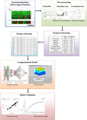
Figure 2. Statistical summary of Extracellular Signal Regulated Kinase protein (a) Kolmogorov-Smirnov plot (b) P-P plot, (c) various statistics values and (d) box plot.

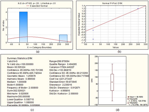
Figure 3. The normal, Kaplan Meier (KM) and Herd Johnson (HJ) method values for the Least Square (LS), and Maximum Likelihood (ML) technique.

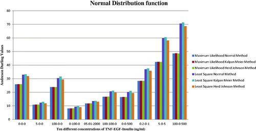
Figure 4. Plots for the Maximum Likelihood technique using normal distribution function.

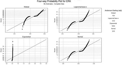
Figure 5. Different plots for the Least Square technique using normal distribution function.

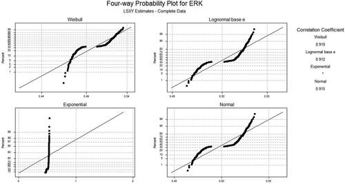
Figure 6. Computational Fuzzy model for predicting cell death /survival.

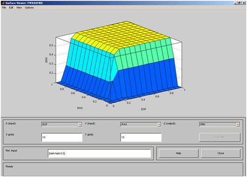
Figure 7. Computational model using Neural Network.

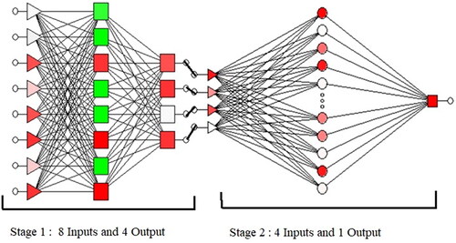
Figure 8. Graph of observed and predicted value.

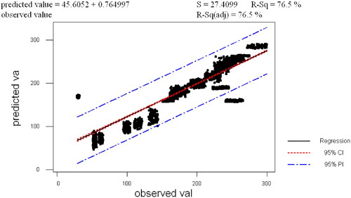
Figure 9. Results of deterministic model using difference equations.

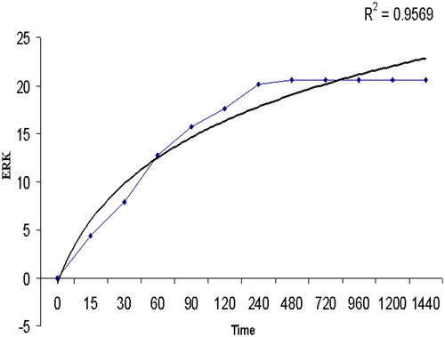
Table 1. Different concentrations of tumour necrosis factor (TNF)-epidermal growth factor (EGF)-insulin.

TNF-EGF-Insulin

0-0-0

5-0-0

100-0-0

0-100-0

5-1-0

100-100-0

0-0-500

0.2-0-1

5-0-5

100-0-500

Table 2. Algorithm for the detection of cell survival/ death.

Start
Step 1: Data is collected from Heat map for three input proteins for ERK protein.
Step 2: Samples were preprocessed using visual tests (P-P plot, Q-Q plot, and box plot), uniformity tests, and Pearson Correlation Coefficients (PCC).
Step 3: Uniformity tests for ERK protein based on the different concentrations and different samples were analysed using different distribution functions and considering different methods such as Normal, Kaplan Meier (KM), and Herd Johnson (HJ).
Step 4: Calculation of the AD values for Maximum Likelihood (ML) and Least Square (LS) technique for different distribution functions were obtained.
Step 5: Detection of cell survival/ death is performed using NN and fuzzy system models.
Step 6: The model is validated by evaluating the predicted value which lies in the range of the observed values.
Step 7: Deterministic model using a differential equation is designed which is in consensus with the proposed model.
End

**The model is validated using the two procedures stated in Step 6 and 7.

Table 3. Pearson correlation coefficient (PCC) for least square method.

	Normal method				Kalpan Meier method				Herd Johnson method
	ND	WD	LND	LD	ND	WD	LND	LD	ND	WD	LND	LD
0-0-0	0.897	0.842	0.910	0.873	0.896	0.848	0.908	0.870	0.899	0.848	0.912	0.878
5-0-0	0.955	0.945	0.950	0.936	0.951	0.949	0.946	0.928	0.956	0.950	0.951	0.940
100-0-0	0.901	0.873	0.878	0.875	0.897	0.877	0.874	0.867	0.903	0.878	0.880	0.880
0-100-0	0.958	0.919	0.959	0.936	0.956	0.925	0.957	0.929	0.960	0.924	0.961	0.940
5-1-0	0.950	0.895	0.955	0.931	0.949	0.901	0.954	0.926	0.952	0.900	0.957	0.935
100-100-0	0.924	0.889	0.925	0.898	0.922	0.895	0.922	0.892	0.926	0.895	0.927	0.903
0-0-500	0.926	0.894	0.913	0.901	0.923	0.899	0.909	0.893	0.928	0.899	0.915	0.905
0.2-0-1	0.886	0.848	0.907	0.861	0.885	0.854	0.905	0.857	0.888	0.854	0.910	0.866
5-0-5	0.838	0.825	0.887	0.814	0.838	0.831	0.885	0.811	0.841	0.831	0.890	0.819
100-0-500	0.820	0.751	0.833	0.797	0.820	0.757	0.833	0.795	0.823	0.756	0.835	0.802

ND: normal distribution function; WD: Weibull distribution function; LND: Lognormal 10 distribution function; LD: logistic distribution function.

Table 4. Correlation values for extracellular signal regulated kinase protein.

Var. X and Var. Y	Mean	Std. Dev.	r (X,Y)	r²	T	p
0-0-0	172.509	37.444
ERK	0.505	0.0209	0.588	0.346	12.563	.000000
5-0-0	167.113	14.425
ERK	0.505	0.0209	0.870	0.758	30.576	.000000
100-0-0	143.494	46.699
ERK	0.505	0.0209	−0.273	0.074	−4.910	.000001
0-100-0	203.120	28.516
ERK	0.505	0.0209	0.822	0.677	24.992	.000000
5-1-0	197.297	18.425
ERK	0.505	0.0209	0.298	0.088	5.391	.000000
100-100-0	143.011	46.890
ERK	0.505	0.0209	0.007	0.000	0.131	.895190
0-0-500	153.181	42.109
ERK	0.505	0.0209	−0.153	0.023	−2.689	.007562
0.2-0-1	236.800	91.738
ERK	0.505	0.0209	0.706	0.499	17.247	.000000
5-0-5	328.767	273.379
ERK	0.505	0.0209	0.630	0.397	14.023	.000000
100-0-500	221.172	96.416
ERK	0.505	0.0209	0.571	0.326	12.014	.000000

Table 5. Kaplan Meier, Normal, and Herd Johnson values using maximum likelihood of the different distribution functions for Extracellular Signal Regulated kinase protein.

	Normal			Weibull			Exponential			Lognormal e			Lognormal 10			Logistic
	NM	KM	HJ	NM	KM	HJ	NM	KM	HJ	NM	KM	HJ	NM	KM	HJ	NM	KM	HJ
0-0-0	25.89	25.95	25.93	25.23	25.32	25.25	88.8	89.0	88.6	22.01	22.05	22.05	22.01	22.05	22.05	23.93	23.87	23.97
5-0-0	10.89	10.91	10.91	7.53	7.55	7.60	115.0	115.3	114.7	12.18	12.20	12.20	12.18	12.20	12.20	10.32	10.46	10.33
100-0-0	23.83	23.90	23.83	25.58	25.66	25.60	65.3	65.4	65.1	30.78	30.85	30.73	30.78	30.85	30.73	21.51	21.70	21.49
0-100-0	8.09	8.11	8.17	8.54	8.57	8.61	101.9	102.1	101.6	7.79	7.80	7.86	7.79	7.80	7.86	7.80	7.80	7.85
5-1-0	11.81	11.81	11.87	13.81	13.84	13.84	113.7	114.0	113.4	10.43	10.42	10.48	10.43	10.42	10.48	11.24	11.16	11.28
100-100-0	16.73	16.78	16.79	16.23	16.29	16.28	64.2	64.3	64.1	16.44	16.48	16.48	16.44	16.48	16.48	15.45	15.48	15.49
0-0-500	16.49	16.54	16.53	16.29	16.35	16.34	73.6	73.7	73.4	20.50	20.56	20.51	20.50	20.56	20.51	15.12	15.23	15.13
0.2-0-1	28.36	28.44	28.40	25.20	25.28	25.22	59.1	59.3	59.0	21.67	21.71	21.71	21.67	21.71	21.71	26.05	26.02	26.09
5-0-5	42.29	42.42	42.30	30.40	30.51	30.41	25.1	25.2	25.1	27.01	27.07	27.04	27.01	27.07	27.04	39.02	39.02	39.05
100-0-500	48.55	48.70	48.53	43.78	43.94	43.75	61.9	62.1	61.8	44.59	44.71	44.57	44.59	44.71	44.57	45.11	45.12	45.13

NM: Normal Method; KM: Kalpan Meier; HJ: Herd Johnson.

Table 6. Anderson Darling values for different distribution functions based on different samples.

Distribution function	Kaplan Meier		Herd Johnson
	Maximum likelihood	Least square	Maximum likelihood	Least square
Weibull function	18.4	18.5	0.923	0.922
Lognormal function	23.2	23.3	0.914	0.908
Exponential function	126.4	127	–	–
Normal function	22.5	22.6	0.916	0.911

Table 7. Comparison of Anderson Darling values for the two different computational models.

Distribution function	Kaplan Meier		Herd Johnson
	Based on samples	Based on concentrations	Based on samples	Based on concentrations
Weibull function	18.4	7.55	0.923	7.6
Lognormal function	23.2	7.8	0.914	7.86
Normal function	22.5	8.11	0.916	8.17

Table 8. Different features of Extracellular Signal Regulated Kinase (ERK).

	ERK	Output
Number of samples	300	300
Minimum	140.711	0.407
Maximum	189.29	0.593
Median	172.221	0.48
Arithmetic mean	167.113	0.483
Standard deviation	14.425	0.051
Variance	208.083	0.003
Coefficient of variation	0.086	0.106

References

- Keskin S. Comparison of several univariate normality tests regarding type I error rate and power of the test in simulation based on small samples. J Appl Sci Res. 2006;2(5):296–300.
- Jain S. Communication of signals and responses leading to cell survival/cell death using engineered regulatory networks [PhD dissertation]. Solan, Himachal Pradesh, India: Jaypee University of Information Technology; 2012.
- Weiss R. Cellular computation and communications using engineered genetic regulatory networks [PhD dissertation]. MIT; 2001.
- Farrell PJ, Rogers-Stewart K. Comprehensive study of tests for normality and symmetry: extending the Spiegelhalter test. J Stat Comput Simul. 2006;76(9):803–816.
- Salau AO, Jain S, Sood M. Computational intelligence and data sciences: paradigms in biomedical engineering. CRC Press; 2022. p. 272. https://www.routledge.com/Computational-Intelligence-and-Data-Sciences-Paradigms-in-Biomedical-Engineering/Salau-Jain-Sood/p/book/9781032123134
- Jain S, Salau AO. An image feature selection approach for dimensionality reduction based on kNN and SVM for AkT proteins. Cogent Eng. 2019;6(1):1–14.
- Kamal MS, Chowdhury L, Khan MI, et al. Hidden Markov model and Chapman Kolmogrov for protein structures prediction from images. Comput Biol Chem. 2017;68:231–244.
- Jain S. Parametric and non-parametric distribution analysis of AkT for cell survival/death. Int J Artif Intell Soft Comput. 2017;6(1):43–55.
- Jain S, Salau AO. Detection of glaucoma using two dimensional tensor empirical wavelet transform. SN Appl Sci. 2019;1(11):1417.
- Normanno N, De Luca A, Bianco C, et al. Epidermal growth factor receptor (EGFR) signaling. Cancer Gene. 2006;366:2–16.
- Jain S, Naik PK, Bhooshan SV. Mathematical modeling deciphering balance between cell death and cell survival using insulin. Netw Biol. 2011;1(1):46–58.
- Jain S, Chauhan DS. Mathematical analysis of receptors for survival proteins. Int J Pharma and Bio Sci. 2015;6(3):164–176.
- Kevin JA, John AG, Suzanne G, et al. A systems model of signaling identifies a molecular basis set for cytokine-Induced apoptosis. Science. 2005;310(5754):1646–1653.
- Salau AO, Jain S. Feature extraction: a survey of the types, techniques, and applications. Proceeding of the 5th IEEE International Conference on Signal Processing and Communication (ICSC); Noida, India; 2019. p. 158–164.
- Jain S. Design of survival-hazard and mathematical model for high osmolarity glycerol protein using parametric and nonparametric methods. Int J Emerg Technol. 2019;10(3):1–9.
- Gaudet S, Janes KA, Albeck JG, et al. A compendium of signals and responses triggered by prodeath and prosurvival cytokines. Mol Cell Proteomics. 2005;4(10):1569–1590.
- Jain S. Compendium model using frequency/cumulative distribution function for receptors of survival proteins: epidermal growth factor and insulin. Netw Biol. 2016;6(4):101–110.
- Salau AO, Jain S. Adaptive diagnostic machine learning technique for classification of cell decisions for AKT protein. Inform Med Unlocked. 2021;23(1):1–9.
- Salau AO, Jain S. Computational modeling and experimental analysis for the diagnosis of cell survival/death for AKT protein. J Genet Eng Biotechnol. 2020;18(1):11.
- Bajzer Z, Myers AC, Vuk-Pavlović S. Binding, internalization and intracellular processing of proteins interacting with recycling receptors. J Biol Chem. 1989;264(23):13623–13631.
- Roberto C, Marcello F, Diego L, et al. Balance between cell survival and death: a minimal quantitative model of tumor necrosis factor alpha cytotoxicity 2009 biological sciences. Biophys Comput Biol. 2009:1–31. https://arxiv.org/abs/0905.4396
- Salau AO, Demilie WB, Akindadelo AT, et al. Artificial intelligence technologies: applications, threats, and future opportunities. Proceedings of the Advances in Computational Intelligence, its Concepts and Applications (ACI 2022); 2022. p. 265–273.