Design and analysis of the location of an online resale business distribution centre in Japan

Abstract

The location of distribution centres for online retailers has become an important issue for many companies. The operation of the distribution centre for e-commerce seems to be different from the traditional concept of distribution centres. This study considers how the location of distribution centres are designed and operated for online retailing using a computer simulation with actual data. This paper analyses current issues in order to propose an effective location for e-commerce distribution centres. An effective location for a multi-distribution system over a wide geographical area is required. This paper clearly points out the importance of locating e-commerce distribution centres over a wide geographical area by performing a computer simulation using actual data on the assumption that online resale business customers live in a metropolitan area. The study created a business model in which a buffer warehouse, which primarily handled commodities with high-frequency shipments, was located near a large consumption area and was used in addition to a large-scale distribution centre. The validity of the created business model was verified by performing a simulation based on actual data. The result revealed that these recommended improvement measures for the location of e-commerce distribution centres can function effectively.

Keywords:

• Distribution centres
• online resale business
• buffer warehouse
• ABC analysis
• transportation planning

1. Introduction

1.1. The aim of this study

The online resale business is one in which commodity transactions are conducted over the Internet, and the purchased commodity is delivered directly to the purchaser. Similar to supermarkets and department stores, the brick-and-mortar company’s distribution centre collects commodities from the multiple distribution centres of their manufacturers and brokers (i.e. wholesalers) and delivers the collected commodities to the company’s stores. The brick-and-mortar company is a company that conducts retail business only at its physical stores.

In the online resale business, frequent shipments of small lots are inevitable. In the brick-and-mortar company, commodities are mainly delivered to its stores just before and after every weekend. Therefore, the delivery characteristics of the online resale business differ greatly from those of the brick-and-mortar company.

If the scheme for the brick-and-mortar company is applied to the online resale business, the delivery cost will increase. Therefore, a new scheme must be proposed for the online resale business. The new scheme is based on a hypothesis that smooth delivery in the last one mile can be achieved by establishing a buffer warehouse in a place near the consumption area.

This study performs a simulation to verify the above-mentioned hypothesis. The simulation allows this study to determine the ratio of the number of commodities handled by a large-scale distribution centre – into which small-scale distribution centres have been consolidated – to the number of commodities handled by a buffer warehouse to minimize the delivery cost. In this study, commodities indicate tangible goods sold in the online resale business, such as books, stationery, daily necessities, clothes, furnishings, pharmaceutical drugs, household electric appliances, and processed foodstuffs.

The aim of this study is to ‘verify the effect of a buffer warehouse in the online resale business’. In the conventional distribution model for the online resale business, a scheme has been adopted in which, by intensively managing inventories and operations in a large-scale physical distribution base (i.e. a distribution centre), duplication in handling large inventories is avoided, inventory compression is attempted, and cost reduction is achieved. However, in this scheme, it has been revealed that the cost of the last one mile for door-to-door delivery is high, so the door-to-door delivery service is constantly unprofitable.

In this study, a new model was designed and proposed in which a buffer warehouse was established in a place near the consumption area, and some of the commodities, with large volumes and high delivery frequencies, were delivered from the buffer warehouse in addition to a large-scale distribution centre where commodities were intensively managed. Moreover, the effect of the new model was verified and confirmed by performing a simulation.

1.2. Background

Recently, the online resale market has greatly expanded; however, to accommodate that growth the logistics system needs to be rebuilt. In the case of retailing, it is believed that there is little difference between the logistic system requirements for online resale businesses and brick-and-mortar companies. However, actually, there is a critical difference between these two types of business entities in terms of the location of their distribution centres. To address this, a sufficient understanding of the differences between brick-and-mortar companies and online resale businesses is required in order to implement an effective logistics system for the online resale market.

This study examines the strategies required to effectively locate distribution centres for an online resale business and deliver goods from those centres to each customer by modelling a logistics system and measuring its improvements using a computer simulation.

The logistics costs for online businesses tend to be higher than those for a brick-and-mortar store with a traditional type of distribution. According to the Japan Institute of Logistics Systems, in Japan the sales logistics costs for all industries averages 4.70%, while the retail industry average, primarily for the delivery from distribution centres to brick-and-mortar stores, which conduct retail business only at its physical stores, is 4.80% (Japan Institute of Logistics System [JILS], 2014). However, sales logistics costs greater than 10% have been reported for many Japanese online retail companies.

One of the factors that contribute to these high costs for online companies is the distribution and home delivery of many small items. Even if small logistical bases are unified into one large-scale distribution centre to create more efficient operations, higher costs resulting from frequent deliveries cannot be avoided. The following cost reduction scheme can be used to improve the logistical efficiency of online retailers (Wakabayashi, Suzuki, Watanabe, & Karasawa, 2014):

(1)	The main distribution centre only focuses on items with a middle- and low-level shipment frequency.
(2)	The small buffer warehouse close to the consumer areas in large cities handles items with high-level shipment frequency and focuses on last-mile delivery and/or end users.
(3)	Most relatively expensive items are shipped from the small buffer warehouse.

After sufficiently understanding the characteristics and features of the online retailing business model, it is necessary to consider the location of the distribution centre and the directionality of the company’s administration and operations.

The location problem is concerned with the optimal location of logistical bases on any given part of a company’s transportation network (Klaptia & Švecová, 2006). Gunasekaran, Ngai, and Cheng (2007) referred to developing an e-logistics system. That is, in previous papers such as Klaptia and Švecová (2006), Gunasekaran et al. (2007), and Hu, Houc, Tiana, and Lia (2015), the necessity of consolidating small-scale distribution centres into a large-scale distribution centre for the online resale business was explained, but the necessity of establishing a buffer warehouse was not described. Simchi-Levi, Kaminsky, and Smichi-Levi (2000) also referred to the importance of one integrated large-scale distribution centre.

Gunasekaran et al. (2007) pointed out only the importance of improving the efficiency of the physical distribution system, of cloud computing-based information systems, and of expanding the scale of a distribution centre. Regarding inventory reduction in the online resale business in particular, the effect of consolidating small-scale distribution centres was discussed.

The idea is that, if small-scale distribution centres can be consolidated into a large-scale distribution centre for the expanded market area of the online resale business, inventory compression can be attained. However, when small-scale distribution centres are consolidated into a large-scale distribution centre, the delivery cost from the large-scale distribution centre to the consumption area increases.

As the theoretical background, the present study develops the model of Bearwood, Hamilton, and Hammersley (1959). The travelling distance between each delivery centre and each delivery destination in a special ward in Tokyo was calculated based on the area of each special ward using the Beardwood-Halton-Hammersley (BHH) theorem.

The number of trucks required for each delivery centre and the travel distance of each delivery centre were obtained based on the maximum loading volume and weight of a truck. The transportation cost (i.e. variable cost) of each delivery centre was obtained while considering overheads. The total transportation cost of each delivery centre was obtained by adding the fixed cost to the variable cost.

Regarding the travelling distance from multiple delivery bases, the delivery area is expressed as A and the number of destinations in the delivery area is expressed as n.

According to the BHH theorem, the minimum travelling distance from a base L_mean and the average travelling distance per delivery destination l_mean are expressed as the following equations:

where β is a constant, β = 0. 765‒0. 72

Here, we consider the case of two bases as the simplest example.

The delivery area A is divided into the first delivery area (area: αA, the number of delivery destinations: αn) and the second delivery area (area: (1−α)A, the number of delivery destinations: (1−α)n).

The minimum travelling distance l₁ is obtained using the BHH theorem.

The minimum travelling distance in the first delivery area is:(1) (2)

The minimum travelling distance in the second delivery area is: (3) (4)

Therefore, the minimum travelling distance in each area decreases in proportion to the value of α (the number of delivery destinations). However, the average travelling distance per delivery destination does not change even though the delivery area is divided into two areas (two delivery bases). Similar results would be obtained even if the number of delivery bases is increased to three or more. In other words, although the number of delivery bases is increased and the delivery area is divided into multiple areas, no advantage is obtained for the delivery distance.

With regard to the delivery time of a truck, when the number of delivery bases increases, the minimum travelling distance decreases and the delivery time also decreases; consequently, customer satisfaction improves. Because the risk of delay and of encountering an accident decreases as the travelling distance decreases, the delivery time, while considering the safety factor, can also decrease as the number of delivery bases increases.

In the present study, the weight and volume of a commodity to be delivered were handled as stochastic quantities. To determine the distribution of the stochastic quantities, an optimal delivery model with multiple delivery bases was examined using beta distribution.

These are the prominent characteristics of the present study. By examining the weight and volume of a commodity to be delivered as stochastic quantities using the probability distribution of commodity volumes and Monte Carlo simulation based on data on the commodities actually handled, it is possible to obtain a realistic optimal delivery model for the number of vehicles required and the delivery cost. The number of vehicles required and the delivery cost can be analysed and examined more precisely when this optimal delivery model is used than when determinism and mean values are used.

One advantage of this present study is that it also paid particular attention to the correlation between the distribution of commodity prices and commodity volumes (i.e. package volumes). It performed a simulation that considered the shape of the distribution of commodity volumes, which govern the number of trucks required and the probability distribution of commodity volumes that were obtained based on the structure of commodity prices.

In the existing studies, Suzuki, Aiura, and Karasawa (2014) examine a reverse logistics network of discarded tires with the simulation which includes a collection system algorithm and cluster-first/route-second method (Kubo, 2001) and local search (Toth & Tramontani, 2008).

In addition, capacitated vehicle routing problems form core of logistics planning, as Chandran and Raghavan (2008) present.

2. Strategies for the location of an online resale business distribution centre

According to Suzuki (2008), the characteristics of recent inventory management strategies for regular, brick-and-mortar stores are:

(1)	Rationalization of forward stock
(2)	Expansion of the selling floor space and minimization of the backyard storage space
(3)	Operation of a large-scale distribution centre

Increasing on-shelf and stock yard inventories without clear strategies is usually inefficient. When commodities are not displayed in stores and, instead, are piled up in backyard storage areas, they may be lost and the amount of work may increase. Therefore, in recent years, retailers have tended to abolish their backyard storage. This tendency may affect the operation of a distribution centre.

When retailers have less stock or no backyard storage, a large-scale distribution centre is required. To construct a system to efficiently and effectively supply the amount of commodities when they are needed, a highly accurate information system is also required.

However, the logistical location conditions between real-shop-delivery and online delivery seems to be different. A minute logistical network from a distribution centre to the home of the end-consumer, with a large quantity of product stock, is required for an online resale business. In addition, a short lead time is required. Therefore, loading efficiency may decrease for each delivery, as the frequency of low-level deliveries may increase from the centre to the end-consumers.

In this case, the transportation cost may be expensive, and, as a result, the total cost for logistics might increase if the delivery is performed with a low loading efficiency at high frequency via trucks. That is why logistics costs greater than 10% have been reported for many Japanese online retail companies, while the retail industry average is 4.80%.

Based on the above information, it is necessary to improve the location of an online resale business distribution centre.

Thus, this paper will address the issues presented above by examining the function of buffer warehouses near large cities and the use of a large nationwide distribution centre, analysing the logistics performance of these centres and evaluating the financial benefits of the proposed solution, and the novelty of this study is that it examines the balance between the delivery cost and the management cost of a distribution centre.

3. Transportation planning from distribution centres to customers

3.1. Transportation planning to customers

To optimize the efficiency and effectiveness of logistical bases, they should be located in specific parts of a company’s transportation network (Klaptia & Švecová, 2006). Okabe and Suzuki (2008) noted that a central logistical hub can be found by calculating the average value of the position coordinates of its delivery points using the density function model that was used by Sala-ngam, Suzuki, Toyotani, and Wakabayashi (2015), which selected the optimal location for a recycling system via a computer simulation. However, as previously mentioned, in addition to one unique hub, at least one more buffer warehouse seems to be required for online resale business.

Thus, in this study, delivery from multiple distribution centres is simulated and the total cost of the transportation plan from the warehouses to each customer as the objective function is calculated. That is, this study considers an optimization problem in an effort to determine the combination of the lots of commodities to be transported from distribution centres to each customer in order to minimize the total transportation cost (objective function) when the amount of commodities to be delivered is given.

Using the total cost for transportation planning from distribution centres to customers as an objective function, an attempt is made to solve a transportation planning problem. Figure 1 shows an outline of this problem.

Figure 1. Transportation planning to customers.

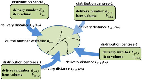
As shown, N is the number of distribution centres: j = 1, 2, ⋯ , N; L_jk is the distance from the distribution centre to the customer; and K_max is the number of commodities to be delivered k = 1, 2, 3, ⋯ , K_k, ⋯ , K_max.

When the delivery from N distribution centres to K_max customers is considered, the total transportation cost (objective function) is expressed as the following equation:(5) (6)

where d_jk is the delivery cost per commodity from distribution centre j to customer k; is the total delivery cost from distribution centre j to customer k; K_jk is the number of commodities to be transported from distribution centre j to customer k; L_jk is the transportation distance from distribution centre j to customer k; is the operating cost of distribution centre j; C_Vj is the variable cost per commodity at distribution centre j; and C_Fjis the fixed cost of distribution centre j.

Here, an optimization problem is considered, which seeks to determine the combination of K_jk (the number of commodities to be transported from distribution centre j to customer k) in order to minimize the total transportation cost (objective function) when K_max (the number of commodities to be delivered) is given.

3.2. Examination of the direct transportation costs from distribution centres to customers

When the number of commodities that can be loaded onto a truck at distribution centre j is expressed as m_jT, the volume of the loaded commodity is expressed as v_ji (I = 1, … … , m_jT), and the maximum loading volume of a truck is expressed as V_Ta, the following equation must be valid:(7)

where indicates the average volume of commodities delivered from distribution centre j. The number of trucks T_j required at distribution centre j is expressed as the following equation: (8)

When the distance from distribution centre j to customer k is expressed as L_jk, the total delivery cost C_jk is expressed as the following equation: (9)

where indicates the fuel cost per km of the travel distance [F_C indicates the average mileage (km/ℓ) of the trucks in operation and C_f indicates the unit cost of the fuel used (yen/ℓ)], C_T indicates the cost to charter a truck, and C_D indicates the labour cost of a driver. When the average travel distance of the trucks at distribution centre j is expressed as , the following equation is valid:(10)

where L_j,k = 1 represents the distance between distribution centre j and the first customer (the entrance of the customer area), L_{j,k = k + 1} represents the distance between the last customer k and distribution centre j, and ΔL_j,k represents the distance between customer k and the next customer k + 1. When i pieces of commodities are delivered to the same customer, the distance between k = k + 1 and k = k + i is calculated as ΔL_j,k = 0. When customers live in a particular area, L_j,k=1 ≅ L_{j,k = k + 1} is valid, and these customers are expressed using the following equation:(11) (12)

The first term on the right side in Equation (8) expresses the effect of the delivery distance, indicating that the direct delivery cost is in proportion to the delivery distance L_jk and the average volume of commodities and in proportion to the square of the number of commodities K_jk to be delivered from distribution centre j. When larger commodities are loaded onto a truck, the number of commodities becomes smaller, the delivery efficiency per truck decreases, the number of necessary trucks increases, and, consequently, the transportation cost increases. Because the transportation cost is in inverse proportion to the maximum loading volume of a truck V_Ta, the use of large trucks seems to be more profitable than the use of small trucks. However, the maximum loading volume of a truck V_Ta and the fuel cost per km κ are in a trade-off relationship. When the accessibility of a truck to deliver a commodity to a customer is taken into consideration, the optimal loading volume of a truck should exist.

The second term on the right side in Equation (8) expresses the effect of the operating cost of trucks, indicating that the size (volume) of a commodity to be delivered affects the direct delivery cost, similar to the first term. Because commodities with various volumes are actually combined, the volume of each commodity v_ji is a stochastic quantity. If Equation (8) is not changed, the number of trucks required at distribution centre j cannot be calculated. Therefore, the combination is determined by assigning weights to the volumes of commodities in order to determine the loading order. Here, commodities are sorted in the order of largest to smallest volume as follows:(13)

By sequentially loading commodities in the order of largest to smallest volume onto trucks at distribution centre j, the number of trucks required at distribution centre j can be determined. By repeating this for distribution centres ranging from j = 1 to j = N, the number of trucks required at all distribution centres to load all commodities can be determined and the number of trucks in operation at each distribution centre can be obtained.

Distribution centres are also sorted in the order of largest to smallest average distance between the centre and customers , and the centre number j is assigned again as follows: (14)

Thus, it is possible to determine all the commodities to be delivered and their associated distribution centres.

Subsequently, the first term of Equation (1) (objective function) is obtained using the number of commodities at each distribution centre K_jk as a variable.

4. Examination of the operating cost of a distribution centre and the total distribution cost

The operating cost of distribution centre is expressed as the following equation:(15)

The operating cost of distribution centre j expressed by the second and third terms of this equation seems to be a function consisting only of the number of commodities K_jk. However, it is necessary to notice that the variable cost per commodity at distribution centre j C_Vj and the fixed cost of distribution centre j C_Fj are functions of the distance from customer L_jk.

In other words, when customers live in a metropolitan area, the cost of the distribution centre rent increases as the centre’s location is closer to the customers. Therefore, the values of C_Vj and C_Fj decrease as the value of L_jk increases. Because K_jk and the direct delivery cost are in a trade-off relationship, optimal K_jk to minimize f₁(K_jk) + f₂(K_jk) may exist.

Based on the above-mentioned consideration, K_jk that minimizes the value of f(K_jk) can be obtained by changing K_jk in Equation (5), which is displayed again as follows:(5)

5. Examination using a simulation

5.1. Background of the simulation

On the basis of the above-mentioned results, we performed a computer simulation using actual data on the assumption that customers of online resale businesses lived in the Tokyo metropolitan area in Tokyo. In the simulation, the online resale business reached customers all over Japan, but its logistical base was located in the Chubu district and commodities were delivered to East and West Japan. To deliver commodities nationwide, a physical distribution base was established in the Chubu district because the distance between the Chubu district and East Japan was almost the same as the distance between the Chubu district and West Japan. In the case where commodities are delivered to Tokyo’s 23 wards from the Chubu district, when there is only one logistical base, the delivery cost using trucks increases with the travelling distance. Therefore, the delivery cost is higher when using a physical distribution base in the Chubu district than when using a distribution warehouse in a place near the Tokyo metropolitan area. Basically, commodities should be shipped out after a specified number of commodities have been collected. However, this case prolongs the lead time from the collection of a commodity to the completion of its delivery. If a large-scale warehouse is located near the Tokyo metropolitan area, the delivery cost of a commodity to West Japan increases.

A system is considered as one of the countermeasures in which a small-scale buffer warehouse is located near the Tokyo metropolitan area, commodities that request frequent shipments of small lots are selected using ABC analysis, and the selected commodities are shipped from the warehouse. The warehouse should focus on commodities with high-frequency shipments. ABC analysis is a method of managing inventoried items in the order of precedence for inventory control and commodity sales.

Namely, inventoried items are classified into A, B, and C, in the order of highest to lowest sales amount, so that inventoried items can be managed efficiently and intensively. In general, 70–80% of the cumulative composition ratio is classified as category A (high-frequency commodities), 80–90% as category B (medium-frequency commodities), and 90–100% as category C (low-frequency commodities).

Based on the above-mentioned system, a simulation was performed in which a distribution centre in the Chubu district (the first centre) and a distribution centre located near the Tokyo metropolitan area (the second centre) were combined as in Figure 2.

Figure 2. Illustrated diagram for the simulation.

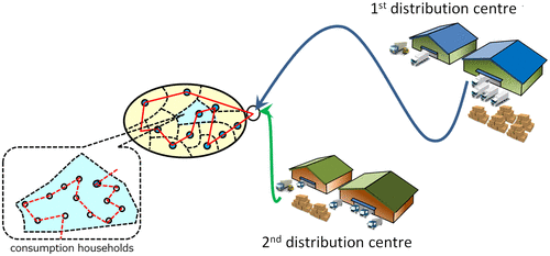
Data on commodity composition, travel distance, the labour cost of a driver, etc. withdrawal and deposit fees, and warehouse charges that were used in the present study were obtained through an interview with a third party logistics company, headquartered in the Chubu District, Japan, which performs online resale business distribution.

5.2. Simulation without considering the probability distribution of the volumes (weights) of commodities (basic case)

First, to understand the rough tendency of delivering commodities, we performed a simulation as a basic case in which the volumes of all commodities were assumed to be of average value, without considering the probability distribution of the volumes of commodities. Figure 3 shows the simulation results. As shown in Figure 3, when the ratio (α) of the first distribution centre was 0.6, the delivery cost was the lowest.

Figure 3. Simulation results obtained using two distribution centres.

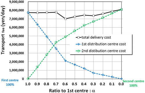
Therefore, to minimize the total distribution cost for delivering commodities in the metropolitan Tokyo area, this study found that the first distribution centre (a unified base in Japan) should be used to some extent and a buffer warehouse should be established in a place near the metropolitan Tokyo area.

5.3. Simulation considering the probability distribution of the volumes (weights) of commodities

In general, a type of probability distribution is observed in the volumes (weights) of commodities to be delivered, and the optimal delivery model is predicted to differ according to the shape of the probability distribution. We paid attention to the correlation between the distribution of commodity prices and commodity volumes (i.e. package volumes), after which we performed a simulation in which the shape of the distribution of commodity volumes – which governed the number of trucks required and the probability distribution of commodity volumes, obtained based on the structure of commodity prices – was taken into consideration.

5.4. Modelling of the distribution of commodity prices

The structure of commodity prices generally differs depending on the specific mail-order company. The present study examines the characteristics of the structure of a company’s selling prices by assuming that the structure of the commodity prices conforms to the beta distribution, which is the probability distribution expressed using two parameters (q and r).

The probability density function of the beta distribution used in the present study is given by the following formula (16):(16)

where expresses the following beta function:

As shown in Figure 4, the characteristics of the beta distribution are that the distribution shape becomes flatter as the values of q and r decrease and steeper as the values of q and r increase. When q > r, the distribution is biased toward the maximum side. When r > q, the distribution is biased toward the 0 side. When q = r = 1, uniform distribution is obtained.

Figure 4. Values of parameter q, r, and the distribution shape.

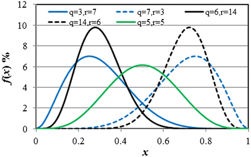
As mentioned above, the beta distribution can be used to create models for various distribution shapes in a finite domain. Therefore, beta distribution can be used to easily examine the structure of various commodity prices.

In addition, the mean value (expected value) M is expressed by the following formula (17):(17)

The variance V is expressed by the following formula (18):(18)

The present study examined a mail-order company whose structure of commodity prices conformed to the beta distribution in which the mean value was 5000 yen and the standard deviation was 4300 yen. By simulating the distribution of commodity prices, the frequency distribution of commodity volumes was estimated. By simulating the delivery of commodities, which conformed to the estimated frequency distribution of the commodity volumes from two distribution centres, several management indices were obtained. The distance between distribution centre 1 and an area for the commodities to be delivered was greater than the distance between distribution centre 2 and the same area. The management indices included delivery costs, each distribution centre’s allocation of sales, carbon dioxide (CO₂) emissions estimated based on the delivery distance, and the delivery delay risk (the traffic accident encounter probability).

5.5. Procedure for obtaining the distribution of the commodity volumes to be delivered based on the simulation results for the distribution of the commodity prices

5.5.1. Determining the distribution of the commodity prices and the simulation

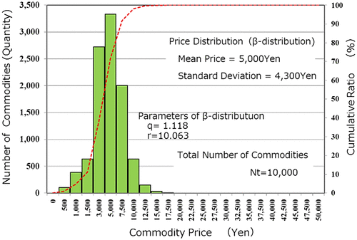
A total of 10,000 random numbers from 0 to 1 were generated and the frequency distribution of the commodity prices that conformed to the beta distribution was formed in which the mean value and the variance of the commodity prices were predetermined. Figure 5 shows the results obtained by simulating the frequency distribution of the commodity prices (the number of commodities), using commodity price P as a variable, in which the mean value and the standard deviation of the commodity prices were 5000 and 4300 yen, respectively. In this figure, the red dotted line indicates the cumulative ratio of the occurrence frequency of the commodity prices (corresponding to the cumulative frequency distribution).

Figure 5. Result of the simulation for distribution of commodity price frequency.

5.5.2. Classifying the commodity prices into four standard commodity price zones

To estimate the commodity volumes based on the commodity prices, the frequency distribution of commodity price P was divided into the following four standard price zones (hierarchies), by which the characteristic distribution of the commodity volumes at each commodity price zone could be presumed:

• Price zone I: 1 ≤ P < 3000 yen

• Price zone II: 3000 yen ≤ P < 10,000 yen

• Price zone III: 10,000 yen ≤ P < 30,000 yen

• Price zone IV: 30,000 yen ≤ P ≤ 50,000 yen (maximum price)

The detailed frequency distribution of the commodity prices obtained from the simulation discussed in the previous section was classified into four standard commodity price zones, according to Commercial Statistics (2015) from the Japanese Ministry of Economy, Trade and Industry. Figure 6 shows the simulation result based on the four standard commodity price zone. In this figure, the cumulative ratio of the frequency is also shown in the red line. When the frequency distribution of the commodity prices obtained from the simulation discussed in Section 5.5.1 was classified into four standard commodity price zones, the price of each commodity was shifted to a price zone that had a specific price range.

Figure 6. Frequency distribution reclassified with standard commodity price zone.

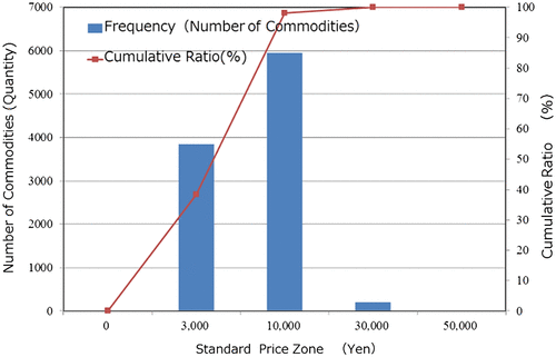
Consequently, information on the price of each commodity obtained by simulating the distribution of the commodity prices was not transferred to the distribution of the commodity volumes. However, since each distribution centre’s allocation of sales, which will be described later, required information on the price of each commodity again, the average price of each standard commodity price zone must be obtained in this stage. In the present study, the average prices of price zones I, II, and II were 2.485, 6371, and 13,038 yen, respectively. Regarding price zone IV, since the probability of occurrence was low and the frequency in the simulation was 0, the average price was assumed to be 40,000 yen.

5.5.3. Estimation of the distribution of the commodity volumes in the four standard price zones

Next, the distribution of the commodity volumes, which was required for simulating the delivery of the commodities, was estimated based on the distribution of the commodity prices. To this end, the commodity volumes in each standard price zone were assumed to form a normal distribution expressed by formula (19), which possessed mean V_m and variance V_ｖ as shown in Table 1.(19)

Table 1. Normal distribution parameters of commodity volumes for four standard price zone.

Price zone	Nominal size	W + L + H (cm)	Horizontal (cm)	Vertical (cm)	Height (cm)	Volume
						Average；Vm (m^3)	Variation coefficient；Vv
30,000 ≤P < 50,000	160 size	152	55.5	45.5	51	0.12879	0.1
10,000 ≤ P <30,000	140 size	132	52.5	40.5	39	0.08292
3000 ≤ P < 10,000	120 size	107.5	43.5	32	32	0.04454
P < 3000	100 size	92	39.5	30	22.5	0.02666

Note: Frequency distribution reclassified with standard commodity price zone.

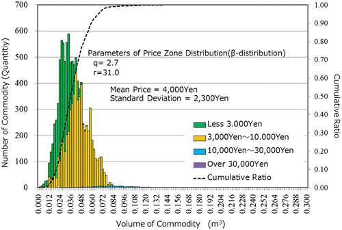
For each standard commodity price zone, several thousand random numbers from 0 to 1 were generated, and the frequency distribution of the commodity volumes in each standard commodity price zone, which was assumed to conform to a normal distribution, was obtained. Using the distribution of the number of commodities shown in each standard commodity price zone, and the distribution of the commodity volumes in each standard commodity price zone, the distribution of the commodity volumes could be simulated .Using the distribution of the number of commodities shown in each standard commodity price zone shown in Figure 5, and the distribution of the commodity volumes in each standard commodity price zone shown in Table 1, the distribution of the commodity volumes could be simulated.

Figure 7 shows the results obtained by simulating the distribution of the commodity volumes using the above-mentioned procedure. In this figure, different colours express different standard commodity price zone shown in Table 1, which indicate the number of commodities at each commodity volume.

Figure 7. Simulation results of commodity volume distribution.

5.6. Delivery simulation

Using the distributions of the commodity volumes and the commodity prices obtained from the process discussed in Section 5.5.1, the delivery of commodities using two distribution centres was examined. The distance between distribution centre 1 and an area for the commodities to be delivered was greater than the distance between distribution centre 2 and the same area. The locations and business expenses, including the fixed and variable costs of the two distribution centres, and the method of simulating the delivery of commodities in the present study, were the same as those included in our previous study. In the present study, the volumes of the commodities to be delivered varied. To examine the effects of the ratio of the number of commodities to be delivered by each distribution centre to the total number of commodities in the management indices, including transportation costs, a delivery simulation was performed in which the ratio of the number of commodities to be shared by distribution centre 1 to the total number of commodities (sharing ratio α) varied.

5.7. Commodity volumes shared by distribution centre 1and its allocation of sales

In performing the delivery simulation, when the distribution of the commodity volumes is simulated again, which is described in the previous chapter, at every sharing ratio α, the random numbers to be generated differ according to each calculation. Moreover, it is difficult to set a specific value for the sharing ratio α. The present study used the method described below as an approximation method.

First, the frequency distribution of the number of commodities at each commodity volume was non-dimensionalised using the total number of commodities. Subsequently, the non-dimensionalised cumulative frequency distribution of the number of commodities against the total number of commodities was obtained. When the vertical axis expressed the commodity volumes and the horizontal axis expressed the non-dimensionalised cumulative frequency distribution of the number of commodities, all the commodities were plotted. Consequently, a graph showing the relationship between the commodity volumes and the sharing ratio α could be obtained in which the vertical and horizontal axes represented the commodity volumes and the sharing ratio α, respectively.

Similarly, by multiplying the average commodity price at each standard commodity price zone, obtained from the process already discussed, and the distribution of commodity volumes, the total value of the commodity prices (corresponding to the sales) could be obtained. When the vertical axis expressed the sales and the horizontal axis expressed the non-dimensionalised cumulative frequency distribution of the number of commodities, all the commodities were plotted. Consequently, a graph showing the relationship between the sales and the sharing ratio α could be obtained in which the vertical and horizontal axes represented the sales and the sharing ratio α, respectively.

Figure 8 shows the relationship between the commodity volumes and the sharing ratio α as well as the relationship between the sales and the sharing ratio α. When these plotted values are expressed by a quadratic function passing through the origin using the method of least squares, formulae (20) and (21) could be obtained, which gave the sharing volume V_C1 and the allocation of sales S_C1 of distribution centre 1, respectively:(20) (21)

Figure 8. Share ratio to first distribution centre and its volume and sales allocation.

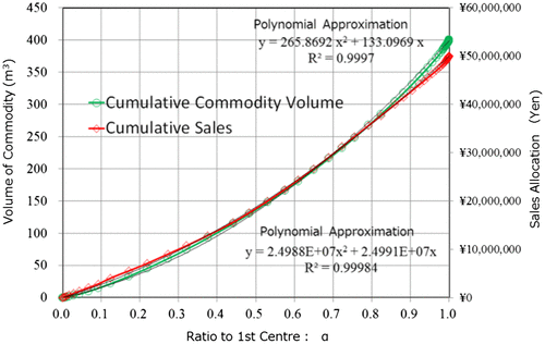
Figure 8 also shows the curves of the commodity volumes and the allocation of sales expressed using formulae (20) and (21), respectively.

5.8. Results of the delivery simulation

By reducing the sharing ratio α in formulae (20) and (21) from 1.0 at intervals of 0.1, the number of commodities to be delivered was shifted from distribution centre 1 to distribution centre 2, and the changes in the number of trucks, the delivery distance, the delivery cost, and the allocation of sales at each distribution centre were investigated.

5.8.1. Distance

Figure 8 shows the relationship between the total travel distance and the sharing ratio α as well as the relationship between the travel distance of the trucks belonging to each distribution centre and the sharing ratio α. These travel distances were obtained by the delivery simulation. When α = 1.0, all of the commodities were delivered by distribution centre 1. When α = 0, all of the commodities were delivered by distribution centre 2.

Because the distance between distribution centre 1 and the area to which the commodities were to be delivered was greater than the distance between distribution centre 2 and the same area, if the amount of commodities shifted from distribution centre 1 to distribution centre 2 increases, the total travel distance will decrease.

The travel distance is proportional to the CO₂ emissions generated by the fuel consumption of the trucks. Therefore, the decrease in the total travel distance has a positive impact on the company’s environmental issues in addition to its management indices, including its transportation costs. A study reported that the traffic accident encounter probability was strongly correlated with the travel distance of the trucks, although it was not proportional. The decrease in the traffic accident encounter probability that results from reducing the travel distance of the trucks is considered to contribute to the prevention of delivery delays.

5.8.2. Transportation costs

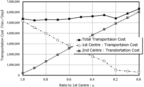
Based on the travel distance of the trucks belonging to each distribution centre, and each centre’s business expenses, the transportation costs were calculated. Figure 9 shows the relationship between the total transportation costs and the sharing ratio α as well as the relationship between the transportation costs of each distribution centre and the sharing ratio α.

Figure 9. Share ratio to first distribution centre α and truck travel distance for each centre.

As shown in this figure, the total transportation costs did not change significantly when approximately 40% of the total number of commodities was shifted from distribution centre 1 to distribution centre 2, although the total transportation costs depended on the methods of setting the values of the fixed costs of each distribution centre and the distribution of the commodity prices.

In this simulation, the management cost of a distribution centre (the first centre) located in the Chubu district and the management cost of a distribution centre (the second centre) located in a place near metropolitan Tokyo were calculated. The transportation cost from the first centre to the consumption area and the transportation cost from the second centre to the consumption area were also calculated. In addition, the ratio of the number of commodities transported from the first centre to the consumption area to the number of commodities transported from the second centre to the consumption area was used as a parameter.

In other words, the total number of commodities delivered per day, the volume and weight of each commodity, the locations of these two distribution centres (i.e. the distances between these two distribution centres and the destination of a commodity), and the fixed costs of these two distribution centres were given as basic input data (i.e. given conditions). Next, the ratio (α) of the number of commodities delivered by the first distribution centre to the total number of commodities was used as a variable, the number of trucks required for each distribution centre, and the travel distance of each distribution centre were obtained based on the maximum loading volume and weight of a truck, the transportation cost (i.e. variable cost) of each distribution centre was obtained while considering overheads, and the total transportation cost of each distribution centre was obtained by adding the fixed cost to the variable cost.

The delivery cost can be reduced by decreasing the ratio of the first distribution centre and increasing the ratio of the second distribution centre (i.e. a buffer warehouse). However, when α exceeds a certain value, the delivery cost cannot be reduced any further. Therefore, the delivery cost can be minimized by obtaining the optimal value of α.

5.8.3. Allocation of sales

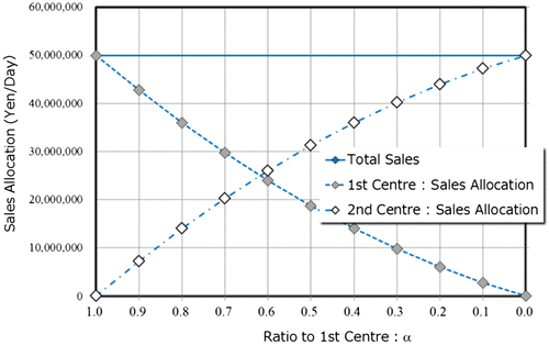
Figure 10 shows the correlationship between the sharing ratio α and the allocation of sales for each distribution centre obtained using formula (17). The transportation costs were subtracted from the sales of each delivery. Figure 11 shows the relationship between the sharing ratio α and the sales of each distribution centre, from which the transportation costs have already been deducted.

Figure 10. Correlation with Share ratio to first distribution centre α and balance of sales and transportation cost.

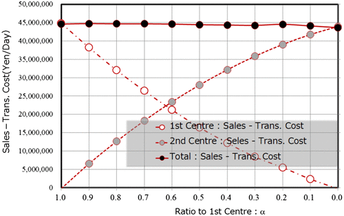
Figure 11. Correlation with share ratio to first distribution centre α and sales allocation.

As shown in this figure, the total number of sales (minus the total transportation costs), decreased very slightly as the number of commodities that were shifted to distribution centre 2 increased. The reason for this was that, when the number of commodities that were shifted to distribution centre 2 exceeded approximately 50%, the total transportation costs slightly increased, as shown in Figure 6.

However, the total number of sales (minus the total transportation costs), remained nearly constant as the number of commodities that were shifted to distribution centre 2 increased to approximately 50%.

Therefore, the shift of approximately 50% of the total number of commodities to distribution centre 2 is considered to effectively reduce the CO₂ emissions and decrease the traffic accident encounter probability of the trucks, which prevents delivery delays.

6. Discussion

In the case of an online resale business where commodities are delivered to the Tokyo metropolitan area from a unified logistical base, if the base is located at a longer distance from the Tokyo metropolitan area, the delivery cost from the base to the Tokyo metropolitan area will be higher than it would be if the delivery distance was shorter. The labour costs, operating costs, and rent for a distribution warehouse are higher if the centre is located near the Tokyo metropolitan area rather than in remote areas. If all of the commodities are delivered from a distribution warehouse located near the Tokyo metropolitan area because the delivery cost is low, the total distribution cost will increase because the cost to maintain the distribution warehouse is high.

To minimize the total distribution cost for delivering commodities to customers in the Tokyo metropolitan area, this study found that the first distribution centre (a unified base in Japan) should be used to some extent and the second distribution centre (a buffer warehouse) should be located near the Tokyo metropolitan area. The ratio of the first distribution centre to the second distribution centre (α) was obtained by performing a simulation based on the consideration described in Chapter 3 and it was found that α = 0.6. Namely, the total distribution cost was the lowest when 60% of the commodities were shipped from the first distribution centre and the remaining 40% were shipped from the second distribution centre.

The case study is just for one distribution centre, and the examination of ‘multiple, large-scale distribution centres + a buffer warehouse’ will be the further research theme.

In general, when multiple, large-scale distribution centres are examined according to similar criteria, the following parameters (1)–(3) are required:

(1)	the distances between each large-scale distribution centre and the final destination of a commodity and between a buffer warehouse and the final destination of a commodity;
(2)	the characteristics of commodities handled by each large-scale distribution centre and the distance between large-scale distribution centres; and
(3)	the ratio of the number of commodities handled by each large-scale distribution centre to the number of commodities handled by a buffer warehouse (α in the submitted manuscript).

Since α increases (α₁, α₂, … , α_n) along with an increase in the number of large-scale distribution centres (n), this relationship must be expressed in a multi-dimensional space. Therefore, the basic computation model must be reconsidered.

In the simplest case, the distance between each large-scale distribution centre and the destination of a commodity can be considered almost the same as the distance between a buffer warehouse and the destination of a commodity. In this case, the relational expressions for the delivery cost of each large-scale distribution centre are the same as the relational expressions for the delivery cost of a buffer warehouse, and also the same model formulation for the delivery cost can be seen.

Therefore, the tendency of the results obtained in this case is considered the same as the tendency of the results obtained in the present study as a whole.

The present study performed a simulation using actual data. The obtained results indicated a general tendency. Even if the locations of multiple delivery centres and the distribution of commodity volumes are different from those used in the present study, an optimal delivery model can be found using the method shown in the present study because the present study generalized these parameters. By examining the weight and volume of a commodity to be delivered as stochastic quantities using the probability distribution of commodity volumes and Monte Carlo simulation based on data on the commodities actually handled, it is possible to obtain a realistic optimal delivery model for the number of vehicles required and the delivery cost. The number of vehicles required and the delivery cost can be analysed and examined more precisely when this optimal delivery model is used than when determinism and mean values are used.

The advantages of establishing a buffer warehouse from the aspect of cost and other quantitative advantages can be summarized as follows:

(1)	In a large metropolitan area, the number of delivery destinations is extremely large. The transportation cost of a commodity is higher if it is transported for a long distance. When a buffer warehouse is established in a large metropolitan area, the established buffer warehouse can handle commodities that require frequent shipments of small lots.
(2)	Because a buffer warehouse can handle urgent shipments and same-day delivery, customer satisfaction improves. This effect cannot be measured by cost performance.
(3)	When the first distribution centre is used for ‘main inventories’, ‘ additional inventories,’ in which commodities that require frequent shipments of small lots are placed.

The optimal delivery model with multiple distribution centres is directly affected by the economic position (fixed cost) of each distribution centre, the distance between each distribution centre and a final delivery destination area, and access to an expressway.

7. Conclusion

Regarding the distribution centre network for the brick-and-mortar company, it can be said that efficiency of delivering commodities can be achieved by consolidating small-scale physical distribution bases into one large-scale base. Regarding the distribution centre network for the online resale business, it is necessary to consider how to cope with the last one mile for door-to-door delivery. To this end, a buffer warehouse that can accommodate request frequent shipments of commodities in small lots must be established in addition to a large-scale distribution centre. That is, the suggestion of the use of a buffer warehouse in the online resale business is novelty of this study.

Regarding online resale businesses, it has been considered effective to deliver commodities nationwide from a large-scale distribution centre instead of multiple bases scattered in the consumption areas, and this method has been adopted. However, the present study created a business model in which a buffer warehouse that mainly handled commodities with high-frequency shipments was located near a large consumption area and that warehouse was used in addition to a large-scale distribution centre. The validity of the created business model was verified by performing a simulation based on actual data. Consequently, it was revealed that the total distribution cost was the lowest when 40% of the commodities were shipped from the buffer warehouse.

Disclosure statement

No potential conflict of interest was reported by the authors.

References

- Bearwood, J., Hamilton, J., & Hammersley, J. (1959). The shortest path through many points. Proceedings of the Cambridge Philosophical Society, 55, 299–327.10.1017/S0305004100034095
- Chandran, Bala, & Raghavan, S. (2008). Modeling and solving the capacitated vehicle routing on trees. In Bruce L. Golden, S. Raghavan, & Edward A. Wasil (Eds.), The vehicle routing problem: latest advances and new challenges (pp. 239–261). New York, NY: Springer.
- Gunasekaran, A., Ngai, E. W. T., & Cheng, T. C. E. (2007). Developing an e-logistics system: a case study. International Journal of Logistics Research and Applications, 10, 333–349. doi:10.1080/13675560701195307
- Hu, Wei, Houc, Ye, Tiana, Longwei, & Lia, Yuan. (2015). Selection of logistics distribution centre location for SDN enterprises. Journal of Management Analytics, 2, 202–215. doi:10.1080/23270012.2015.1077481
- Japan Institute of Logistics System. (2014). Buturyu Cost Hokokusho 2014 nendo [Logistics Cost Annual Report 2014]. Tokyo: Japan Institute of Logistics System.
- Klaptia, Vladimír, & Švecová, Zuzana. (2006). Logistics centres location. Transport, 21, 48–52. doi:10.1080/16484142.2006.9638041
- Kubo, M. (2001). Logistics Kogaku [Logistics engineering] (pp. 111–116). Tokyo: Asakura Shoten.
- Ministry of Economy, Trade and Industry. (2015). Commercial statistics. Tokyo: Association of Commercial Statistics.
- Okabe, Atsuyuki, & Suzuki, Atsuo. (2008). Saitekihaichi no Suuri [Mathematics for optimal relocation]. Tokyo: Asakura Publishing.
- Sala-ngam, Sarinya, Suzuki, Kuninori, Toyotani, Jun, & Wakabayashi, Keizou. (2015). A study on the location selection of industrial wastes treatment facilities in Chiba, Japan. In V. Kachitivichyanukul, K. Sethanan, & P. Golinska-Dawson (Eds.), Toward sustainable operations of supply chain and logistics systems pp. 2007–2219). Heidelberg: Springer.
- Simchi-Levi, David, Kaminsky, Philip, & Smichi-Levi, Edith. (2000). Designing and managing the supply chain: Concept, strategies, and case studies. New York, NY: McGraw-Hill.
- Suzuki, Kuninori. (2008). Shohin Kanri Buturyu Kanri [Product management and logistics management]. Tokyo: Nikkan Kougyou Shimbunsha Publishing.
- Suzuki, Kuninori, Aiura, Nobunori, & Karasawa, Yutaka. (2014). A consideration on an effective reverse logistics system for discarded tires. In P. Golinska (Ed.), Logistics operations, supply chain management and sustainabiliy (pp. 285–292). Heidelberg: Springer.
- Toth, Paolo, & Tramontani, Andra. (2008). An integer linear programming local search for capacitated vehicle routing problems. In L. Golden Bruce, S. Raghan, & A. Edward (Eds.), The vehicle routing problem: Latest advance and new challenges (pp. 275–295). New York, NY: Springer.
- Wakabayashi, Keizou, Suzuki, Kuninori, Watanabe, Akihiro, & Karasawa, Yutaka. (2014). Analysis and suggestion of an e-commerce logistics solution. In P. Golinska (Ed.), Logistics operations, supply chain management and sustainabiliy (pp. 285–292). Heidelburg: Springer.