Multivariate control chart based on PCA mix for variable and attribute quality characteristics

ABSTRACT

Two types of control charts exist based on different quality characteristics: variable and attribute. These characteristics are commonly monitored using separate procedures. Only a few studies focused on the utilization of control charts to monitor a process with mixed characteristics. This study develops a new concept of the control chart based on a Principal Component Analysis (PCA) Mix, that is a PCA method that can jointly handle continuous and categorical data. The Kernel Density Estimation (KDE) method is used to estimate the control limit. Through simulation studies, the performance of the proposed chart is evaluated using the Average Run Length (ARL). control limits obtained from KDE produce a stable ARL₀ at ~ 370 for For the shifted process, the proposed chart demonstrates excellent performance for an appropriate number of principal components used. Applications of the simulated process and real cases show that the proposed chart is sensitive to monitoring the shifted process.

KEYWORDS:

• Mixed chart
• PCA mix
• T² control chart
• kernel density estimation
• average run length

1. Introduction

One of the most powerful tools in Statistical Process Control (SPC) is the control chart, which has been widely used in industries and services. Based on the type of monitored quality characteristics, there are two kinds of control charts: variable (interval or ratio) and attribute (category) (Montgomery, 2009). The variable control chart is appropriate to use if the quality characteristics of the product are measured on a numerical scale such as weight and height. On the other hand, if the quality characteristics are not measured on a numerical scale (in categorical form) such as color and softness, an attribute control chart can be employed (Sorooshian, 2013). The control chart is not only developed for the univariate case but also for the multivariate case where each characteristic cannot be monitored separately. Therefore, multiple quality characteristics should be monitored together using a multivariate control chart.

The recent development of the multivariate control chart based on the Shewhart approach includes robust Hotelling’s T² control chart (Abu‐Shawiesh, Kibria, & George, 2014; Ahsan, Mashuri, & Khusna, 2018; Alfaro & Ortega, 2009; Ali, Syed Yahaya, & Omar, 2013), fuzzy Hotelling’s T² control chart (Alkindi, Mashuri, & Prastyo, 2016), Hotelling’s T² control chart based on a Markov Chain approach (Seif, Faraz, Saniga, & Heuchenne, 2016), Hotelling’s T² control chart based on Principal Component Analysis (PCA) (Kim & Lee, 2003; Kourti, 2005; Phaladiganon, Kim, Chen, & Jiang, 2013), and the Shewhart chart for monitoring the coefficient of variation for short production (Amdouni, Castagliola, Taleb, & Celano, 2017).

Meanwhile, the recent development of the Multivariate Cumulative Sum (MCUSUM) procedure has been studied for autocorrelated data (Noorossana & Vaghefi, 2006), Artificial Neural Networks (ANNs) (Arkat, Niaki, & Abbasi, 2007), and Support Vector Regression (Issam & Mohamed, 2008). The Multivariate Exponentially Weighted Moving Average (MEWMA) approach was studied by Chen, Cheng, and Xie (2005) for simultaneously monitoring mean and variance. Pirhooshyaran and Niaki (2015) and Khusna, Mashuri, Suhartono, Prastyo, and Ahsan (2018) used the MEWMA approach for autocorrelated data, while Gunaratne, Abdollahian, Huda, and Yearwood (2017) adopted this approach to monitor the process variability for high-dimensional data. By contrast, a multivariate control chart based on attribute characteristics was developed for multiattribute processes (Chena, Chang, & Chen, 2011; Cozzucoli, 2009; Mukhopadhyay, 2008; Niaki & Abbasi, 2007a, 2007b; Wibawati, Mashuri, Purhadi, Irhamah, & Ahsan, 2018; Wibawati, Purhadi, & Irhamah, 2016), and for multivariate Poisson distributions (Chiu & Kuo, 2008; Laungrungrong, 2010; Niaki & Khedmati, 2013; M. Aslam, Srinivasa Rao, Ahmad, & Jun, 2017).

From a literature review of multivariate control charts by Lowry and Montgomery (1995), Umit and Cigdem (2001), Bersimis, Psarakis, and Panaretos (2007), and Bersimis, Sgora, and Psarakis (2016), there have been only few research-studied control charts that monitor mixed processes composed by variable and attribute characteristics, called a mixed control chart. Meanwhile, a mixed monitoring scheme is sometimes necessary in the manufacturing process (Pu, Li, & Xiang, 2011). Aslam, Azam, Khan, and Jun (2015) proposed a mixed control chart using combined and np procedures to monitor the process, and found it more efficient than the conventional chart. Aslam, Khan, Aldosari, and Jun (2016) presented two mixed control charts using EWMA statistics and Hybrid Exponential Weighted Moving Average (HEWMA) statistics by assuming that the quality characteristic follows the normal distribution. The performance of these two charts was compared with that of the mixed chart. The HEWMA chart has the ability to detect a small shift in the process and outperforms EWMA and mixed charts. Khan, Aslam, Kim, and Jun (2017) proposed a mixed control chart for a life test by assuming that the quality characteristics follow the Weibull distribution. However, those studies are only for a univariate case which is decomposed into variables and attributes and simultaneously monitored using a single control chart. In fact, the process can be monitored separately using either a variable chart or attribute chart without using a mixed chart.

A problem arises when the actual process comes from two different quality characteristics which cannot be monitored using an existing mixed chart. PCA Mix is a method that can handle different types of quality characteristics using a combination of Principal Component Analysis (PCA) and Multiple Correspondence Analysis (MCA). PCA Mix was first proposed by De Leeuw and Van Rijckevorsel (1980) and was later developed by Kiers (1988, 1989, 1991) and Chavent, Kuentz-Simonet, Labenne, and Saracco (2014). Although PCA Mix can be employed for different types of quality characteristics, the distribution of Principal Component Scores (PCs) produced by PCA Mix does not follow a multivariate normal distribution or even unknown distribution. Consequently, a conventional T² control chart constructed by PCA Mix generates many false alarms because it assumes a multivariate normal distribution. To overcome this issue, a Kernel Density Estimation (KDE) can be employed to calculate the control limit (Ahsan, Mashuri, Kuswanto, Prastyo, & Khusna, 2018; Chou, Mason, & Young, 2001; Phaladiganon, Kim, Chen, Baek, & Park, 2011; Phaladiganon et al., 2013).

The key contribution of this paper lies in forming a new procedure for monitoring the mixed characteristics in a single chart. To date, the product in a manufacturing process is only monitored using one of the characteristic types measured (only considering variable or attribute characteristics). If both characteristics are monitored, this is commonly done using separate procedures. This actually becomes ineffective because it needs to see the results from the two different procedures before finally making a decision on the quality of the product. For example, when the length and weight of a product have been stated in an in-control condition, it is also necessary to analyse the defects and level of softness from the product using different procedures. If the monitoring results of the two procedures give different results, the decision-maker will have difficulty in determining the quality of the product. Maybe the product will be declared as in-control if the two procedures produce the same results, or the decision-maker will prefer the results from one procedure when the two procedures yield different outcomes.

Based on the aforementioned reasons, this paper focuses on developing a new approach to monitor a process with a mixture of variable and attribute characteristics. This new approach is expected to simplify the monitoring process without reducing the level of precision and accuracy. A multivariate T² control chart based on PCA Mix is proposed, while KDE is employed to estimate its control limit. The performance of the proposed chart with a control limit calculated using KDE is compared with a proposed chart that employs conventional F distribution to calculate the control limit using the Average Run Length (ARL). Moreover, the application of the proposed chart to monitor simulated and real case data is presented in this study. This paper is organized as follows. Section 2 describes the charting procedure of a T² chart based on PCA Mix. Section 3 presents some simulation studies. Next, the application of the proposed chart for simulated data and real cases is displayed in section 4. The managerial implications of the proposed chart are discussed in section 5. Finally, section 6 summarizes the obtained results.

2. Charting procedures

2.1. PCA mix

Multivariate data analysis can be described as statistical methods to analyse data consisting of two or more quality characteristics. These quality characteristics can be either variable (interval or ratio) or attribute (category). PCA is one of the statistical methods for the dimensional reduction of continuous data, which in SPC are referred to as variable characteristics. MCA is an extension of Correspondence Analysis (CA) and is used to analyse the relationship pattern of several correlated categorical variables, which in SPC are referred to as attribute characteristics. MCA can be viewed as a generalization of the PCA method when the observations are categorical (Jolliffe, 2002). Thus, the different types of quality characteristics can be handled together by using the PCA Mix method as a combination of PCA and MCA.

The PCA Mix procedure used in this paper follows the approach proposed by Chavent et al. (2014). Let matrix and matrix consist of variable and attribute characteristics, respectively, where n is the number of observations, p is the number of variable characteristics, and q is the number of attribute characteristics. An indicator matrix with dimensions contains binary coding from each level of attribute characteristics, where m is the number of total levels of attribute characteristics. An matrix consists of a real number element, where and are centred matrices of and . is calculated as

(1)

where is the weights of the rows of Z, is the weights of the columns of Z, the first p columns of Z are weighted by 1, and the last m columns are weighted by for The next step is solving the eigenvalue problem of using the Generalized Singular Value Decomposition (GSVD) in Chavent et al. (2014) as

(2)

where where are the eigenvalues of and r denotes the rank of Matrix , which has dimensions, is an eigenvector of , and is the matrix of the eigenvectors of Thus, the principal component of PCA mix can be computed as

(3)

with the size of

2.2. Kernel density estimation

The kernel is a weighting function commonly used in nonparametric techniques. The kernel estimator was first introduced by Murray Rosenblatt (1956) and Parzen (1962) and was called the Rosenblatt-Parzen kernel density estimator. Chou et al. (2001) introduced KDE to estimate the distribution of statistics. Given n values of statistics obtained from an in-control condition, the empirical density of T² can be expressed using the following kernel function:

(4)

where K and are the kernel function and estimated smoothing parameter, respectively.

Furthermore, the control limit of based on KDE can be determined by the percentile of kernel distribution (Phaladiganon et al., 2011). The cumulative distribution function for KDE can be written as

(5)

Thus, the control limit of T² based on KDE is the th percentile of the empirical density of , as follows:

(6)

The integral in equation (5) is not simple to solve owing to the complication of the kernel function. Thus, the trapezoidal rule (Burden & Faires, 2011), one of the numerical integration methods to approximate the definite value of an integral equation, is used to solve the kernel control limit.

2.3. T² control chart based on PCA

The conventional T² control chart is constructed based on PCA uses the first k PCs. The statistic of the chart based on PCA can be computed by using the following formula:

(7)

where the first k PCs are , and is the eigenvalue corresponding to the v-th PC. Under the assumption that the data follow a multivariate normal distribution, the control limit of a PCA-based T² control chart can be obtained as follows:

(8)

where n is the number of observations, k is the number of PCs retained, and is the false alarm rate.

2.4. T² control chart based on PCA mix

In this research, a control chart is constructed based on PCA Mix with KDE using the PCs obtained from PCA Mix, which is denoted as in equation . The proposed multivariate control chart is constructed by statistics for the first k PCs of The T² statistic for PC Mix, which is denoted by is calculated as follows:

(9)

where , is an eigenvalue that corresponds to the vth PCs from the in-control process; and is the mean vector of the in-control process. Furthermore, the control limit of the proposed chart is calculated using the KDE method because the distribution of the statistic is unknown. The Gaussian KDE of the statistic is estimated as follows:

(10)

where the Gaussian kernel is defined as

(11)

Moreover, the distribution function of that is denoted by is calculated by

(12)

is calculated using the trapezoid rule method as follows:

(13)

where and are the minimum and maximum value of Hence, the control limit of based on KDE is the th percentile and is calculated as follows:

(14)

Furthermore, the established control limit is used to monitor new observations.

3. Simulation studies

In this section, several simulation studies are conducted to investigate the distribution of to determine the control limit of the proposed chart, and to evaluate its performance. The variable characteristics are assumed to follow the multivariate normal distribution Meanwhile, the attribute characteristics follow the multinomial distribution The number of variable characteristics p used in this study are 5, 10, and 30; the number of principal components is k; and the number of observations n = 1000. One attribute characteristic follows the multinomial distribution used in this study. There are three scenarios for values of : (1) (2) (3) The combinations parameters represent the slightly balanced class in the attribute characteristics, while the others represent imbalanced as well as extreme imbalanced classes. Furthermore, the KDE is used to calculate the control limit, and the ARL is used to evaluate the performance of the proposed chart. The ARLs are calculated through a simulation process for 1000 replications.

3.1. Distribution of

The simulation study in this section investigates whether the distribution of PC Mix follows the multivariate normal. The variable characteristics are generated by a multivariate normal distribution with mean vector and covariance matrix . The attribute characteristics are generated by a multinomial distribution with three types of parameter, as mentioned previously.

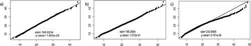
Figure 1 shows a Q-Q plot of PC Mix for p = 5 and k = 4 with and Figure 2 illustrates the Q-Q plot of PC Mix for p = 10 and k = 5. Meanwhile, Figure 3 displays the Q-Q plot of for p = 30 and k = 20. From these figures, it can be seen that the distribution of PC Mix does not follow the multivariate normal distribution confirmed by the statistic and the p values of a Royston multivariate normal test. However, there is an indication that the distribution of PC Mix will follow the multivariate normal distribution when the number of quality characteristics increases while the parameter for the attribute characteristic is balanced at (see Figure 3). The distribution of PC Mix deviates from a multivariate normal distribution when the parameter for the attribute characteristic is imbalanced, for example, when as well as . These results are also supported by increasing the p-value when the number of quality characteristics is increasing and the parameters of the attribute characteristics are balanced.

Figure 1. The Q-Q plot of first four PCs Mix with p = 5 for: (a) , (b) , (c) .

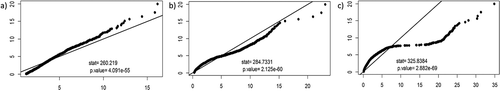
Figure 2. The Q-Q plot of first five PCs Mix with p = 10 for: (a) , (b) , (c) .

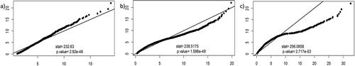
Figure 3. The Q-Q plot of 20 first PCs Mix with p = 30 for: (a) , (b) , (c) .

In order to prove these findings, four statistical methods for multivariate normal distribution testing are employed: Mardiah, Henze-Zirkler, Royston, and Generalized Shapiro-Wilk. This simulation is repeated 1,000 times for various combinations of p, k, and values of . Furthermore, the probability of failing to reject the null hypothesis for each combination is calculated.

Table 1 shows the probability of PCs to follow a multivariate normal distribution. In this simulation, various p and k are combined with to calculate the probability. The simulation process reveals that all combinations produce a zero probability of following a multivariate normal distribution. However, there is still a possibility that PCs will follow a normal multivariate distribution when using very large p and k as well as the balanced parameter of the attribute characteristics.

Table 1. Probability of PCs Mix to follow multivariate normal distribution for 1000 replications.

p	k	Parameter of Attribute Characteristics	Normality test Method
			Mardiah	Henze-Zirkler	Royston	Generalized Shapiro-Wilk
5	2		0	0	0	0
			0	0	0	0
			0	0	0	0
	3		0	0	0	0
			0	0	0	0
			0	0	0	0
	4		0	0	0	0
			0	0	0	0
			0	0	0	0
10	3		0	0	0	0
			0	0	0	0
			0	0	0	0
	5		0	0	0	0
			0	0	0	0
			0	0	0	0
	7		0	0	0	0
			0	0	0	0
			0	0	0	0
30	5		0	0	0	0
			0	0	0	0
			0	0	0	0
	10		0	0	0	0
			0	0	0	0
			0	0	0	0
	15		0	0	0	0
			0	0	0	0
			0	0	0	0
	20		0	0	0	0
			0	0	0	0
			0	0	0	0

The next simulation study investigates the empirical distribution of that is used in this research. The purpose of the investigation is to compare the empirical distribution of and conventional T² -based on PCA through a simulation process. The KDE method is employed to visualize the density of these statistics.

Figure 4 shows an empirical density comparison of T² based on PCA and for p = 5 and k = 4 on the left-hand side, and for p = 10 and k = 5 on the right-hand side. The empirical density of the T²-based PCA is represented by a black line, while for it is represented by a red line. The figure illustrates the difference in empirical density between the and T²-based PCA charts. For the distribution of the statistic, two modes are found, indicating that the statistic of has a mixture distribution. These two modes cannot be depicted clearly for balanced parameters (see Figure 4a). However, these two modes are clearly seen for imbalanced and extreme imbalanced parameters of the attribute characteristics (see Figures 4b and 4c).

Figure 4. Comparison of empirical density of T² and for: p = 5 and k = 4 (left) and p = 10 and k = 5 (right).

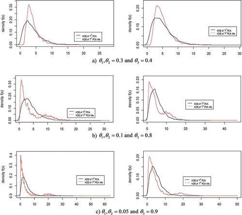
From these investigations, it can be concluded that PC Mix does not follow a multivariate normal distribution, nor does its statistic follow the F distribution that the conventional T²-based PCA chart does. Hence, it is not appropriate to use the assumption of multivariate normal for this proposed chart.

3.2. Control limit

The findings in section 3.1 proved that PC Mix does not follow a multivariate normal distribution and that its statistic does not follow an F distribution. As a result, KDE is employed in order to estimate an unknown distribution. The control limit of needs to be estimated using both the KDE method and conventional F distribution as in equation in order to compare the performance of these control limits by using ARL₀ criteria.

Table 2 presents a comparison of control limits with its ARL₀ using the KDE method and an F distribution. Since the simulation study is conducted using a significance level 0.00273 that corresponds to a theoretical ARL₀ of 370, the control limits using the KDE method are more reliable than those using an F distribution. For several combinations of p, k, and parameters of attribute characteristics, the control limits using the KDE method always produce an empirical ARL₀ at about 370. Meanwhile, the ARL₀ of the control limits using an F distribution is not stable. However, for and the parameter of attribute variables , both the ARL₀ and the control limit using the KDE method are coincidentally similar to those using an F distribution.

Table 2. Comparison of control limit and ARL₀ between KDE and Conventional Method.

0.00273 (370)		KDE	F Dist	KDE	F Dist	KDE	F Dist
p = 5 k = 2	CL	3.629071	11.90081	13.16541	11.90081	19.82783	11.90081
	ARL0	383.134	1000	374.736	154.801	374.092	21.602
p = 5 k = 3	CL	11.14456	14.26894	15.83102	14.26894	24.62383	14.26894
	ARL0	357.994	799.82	366.513	164.407	364.804	14.627
p = 5 k = 4	CL	13.97892	16.40835	18.19012	16.40835	26.55745	16.40835
	ARL0	368.043	711.333	388.796	174.176	358.438	13.831
p = 10 k = 3	CL	11.29925	14.26894	16.19714	14.26894	22.58088	14.26894
	ARL0	376.017	795.165	368.771	147.328	365.733	25.407
p = 10 k = 5	CL	16.33098	18.41051	20.17838	18.41051	27.97997	18.41051
	ARL0	361.116	648.978	376.466	186.247	376.07	22.675
p = 10 k = 6	CL	18.35027	20.31917	21.68706	20.31917	29.38881	20.31917
	ARL0	368.203	620.895	365.344	188.343	387.29	21.881
p = 10 k = 7	CL	20.38013	22.1592	23.73523	22.1592	31.73267	22.1592
	ARL0	369.308	565.435	375.269	208.362	376.87	26.543
p = 30 k = 10	CL	25.67681	27.40177	28.34902	27.40177	34.06427	27.40177
	ARL0	366.619	540.46	374.484	262.467	382.573	64.32
p = 30 k = 15	CL	33.69125	35.59768	35.90885	35.59768	42.17232	35.59768
	ARL0	372.149	541.459	374.561	318.415	382.387	74.517
p = 30 k = 20	CL	41.15506	43.42942	43.34664	43.42942	49.38334	43.42942
	ARL0	367.621	569.555	365.355	371.901	371.077	89.721

3.3. Performance of proposed chart

This section provides a performance evaluation of the proposed control chart using the KDE method. The out-of-control ARL is calculated by adding a shift for each variable characteristic where and the attribute characteristics are shifted by where . Three kinds of numbers of PCs (representing low, moderate, and high) are evaluated for each number of variable characteristics. Moreover, the KDE control limits for several combinations of p, k, and the parameter of the attribute characteristic are taken from Table 2. A simulation study is conducted using significance level 0.00273 that corresponds to a theoretical ARL₀ of 370. The empirical values of ARL₀ obtained from the simulation studies are presented in Table 4–7.

Table 3. ARLs for with several combinations of p and k.

Shift		p = 5	p = 5	p = 5	p = 10	p = 10	p = 10	p = 30	p = 30	p = 30
		k = 2	k = 3	k = 4	k = 3	k = 5	k = 7	k = 10	k = 15	k = 20
0.0	0.0000	383.1	358.4	355.5	361.2	355.0	369.1	359.6	362.3	362.7
0.1	0.0025	333.4	327.7	340.0	330.7	319.8	347.6	315.9	316.4	315.8
0.2	0.0050	197.6	254.8	268.8	271.4	279.4	277.3	249.1	249.6	241.4
0.3	0.0075	19.3	265.4	252.8	321.8	259.8	249.5	143.4	163.3	133.2
0.4	0.0100	7.2	311.9	270.8	140.0	180.2	190.2	71.0	91.6	66.4
0.5	0.0125	5.1	176.0	186.5	61.3	95.5	125.9	31.8	46.1	32.5
0.6	0.0150	3.8	102.9	130.1	29.5	60.3	74.4	15.8	22.9	15.2
0.7	0.0175	3.0	56.7	85.7	15.7	32.1	45.2	7.2	11.4	7.5
0.8	0.0200	2.4	34.1	51.9	9.2	19.7	26.8	4.1	6.4	4.0
0.9	0.0225	1.9	19.9	34.7	5.7	11.6	17.4	2.5	3.5	2.5
1.0	0.0250	1.7	13.6	22.8	3.5	7.0	10.9	1.6	2.2	1.7
1.1	0.0275	1.5	8.7	14.9	2.6	4.8	6.7	1.3	1.5	1.3
1.2	0.0300	1.3	6.5	10.5	1.9	3.3	4.7	1.1	1.3	1.1
1.3	0.0325	1.2	4.8	7.2	1.6	2.4	3.3	1.0	1.1	1.0
1.4	0.0350	1.2	3.5	5.6	1.3	1.9	2.6	1.0	1.1	1.0
1.5	0.0375	1.1	2.7	4.0	1.2	1.5	2.0	1.0	1.0	1.0

Table 4. ARLs for with several combinations of p and k.

Shift		p = 5	p = 5	p = 5	p = 10	p = 10	p = 10	p = 30	p = 30	p = 30
		k = 2	k = 3	k = 4	k = 3	k = 5	k = 7	k = 10	k = 15	k = 20
0.0	0.0000	372.8	378.3	386.0	376.7	368.5	381.5	371.7	374.6	371.3
0.1	0.0025	295.3	305.1	336.8	351.0	313.4	319.1	313.8	306.4	327.1
0.2	0.0050	448.8	214.9	257.6	287.2	234.4	240.0	172.5	184.7	199.7
0.3	0.0075	415.9	153.8	176.9	184.2	144.7	153.2	117.0	125.5	149.7
0.4	0.0100	303.6	109.2	137.7	95.4	76.3	81.7	72.4	86.8	92.2
0.5	0.0125	284.1	46.1	51.4	66.4	50.1	57.0	43.0	50.4	57.7
0.6	0.0150	149.6	31.5	32.4	42.5	33.8	38.3	23.0	28.6	34.9
0.7	0.0175	84.1	24.6	24.0	28.4	24.9	29.0	13.0	16.6	20.1
0.8	0.0200	48.0	19.2	17.8	19.9	18.3	19.9	7.6	10.7	12.5
0.9	0.0225	28.7	15.2	14.5	14.3	13.7	15.1	5.0	6.2	7.8
1.0	0.0250	17.7	12.9	11.8	9.9	10.0	11.7	3.0	4.0	4.9
1.1	0.0275	13.6	11.0	10.4	7.9	8.4	9.4	2.2	2.6	3.4
1.2	0.0300	10.5	9.3	9.0	6.0	7.0	8.1	1.6	2.0	2.4
1.3	0.0325	8.7	8.7	8.5	4.6	5.8	6.3	1.3	1.5	1.8
1.4	0.0350	7.1	7.3	7.8	3.6	4.8	5.4	1.1	1.2	1.4
1.5	0.0375	6.2	7.4	7.5	2.8	3.7	4.4	1.0	1.1	1.2

Table 5. ARLs for with several combinations of p and k.

Shift		p = 5	p = 5	p = 5	p = 10	p = 10	p = 10	p = 30	p = 30	p = 30
		k = 2	k = 3	k = 4	k = 3	k = 5	k = 7	k = 10	k = 15	k = 20
0.0	0.0000	370.9	393.5	340.6	392.3	366.8	398.8	395.7	382.4	366.6
0.1	0.0025	382.2	358.7	259.8	429.9	292.2	312.0	325.4	317.2	296.1
0.2	0.0050	662.6	368.7	192.3	414.6	216.2	215.6	86.1	92.4	84.5
0.3	0.0075	655.3	352.6	132.0	240.1	106.4	95.0	57.6	62.3	59.1
0.4	0.0100	472.9	232.1	76.2	37.9	24.2	24.7	36.7	39.6	38.1
0.5	0.0125	26.6	30.9	17.2	22.6	21.8	18.6	24.8	26.1	28.0
0.6	0.0150	16.4	20.1	15.5	18.0	16.9	16.3	20.3	19.9	21.2
0.7	0.0175	15.6	17.0	15.1	16.4	16.1	16.2	17.4	17.9	17.1
0.8	0.0200	16.5	16.5	16.1	16.8	16.7	16.3	14.4	15.0	16.3
0.9	0.0225	18.7	18.8	17.5	17.8	17.6	17.5	12.9	13.5	14.6
1.0	0.0250	20.5	19.4	19.7	19.4	19.7	19.8	8.5	11.5	12.7
1.1	0.0275	21.6	20.9	23.1	22.0	21.2	22.8	5.3	7.7	8.8
1.2	0.0300	25.4	26.0	24.3	22.9	24.7	24.8	3.3	4.7	5.8
1.3	0.0325	27.4	29.3	28.5	21.9	25.9	26.3	2.1	2.9	3.9
1.4	0.0350	35.3	33.7	31.2	21.0	25.4	26.8	1.6	1.9	2.4
1.5	0.0375	38.6	37.9	38.8	14.8	23.1	29.0	1.2	1.5	1.7

Table 6. ARLs of control chart with k that can explain 70% of total variance for several p.

Shift
		p = 5 k = 4	p = 10 k = 6	p = 30 k = 15	p = 5 k = 4	p = 10 k = 6	p = 30 k = 15	p = 5 k = 4	p = 10 k = 6	p = 30 k = 15
0	0	355.5	365.0	362.3	386.0	364.0	374.6	340.6	365.0	382.4
0.1	0.0025	340.0	337.0	316.4	336.8	299.0	306.4	259.8	294.0	317.2
0.2	0.005	268.8	255.0	249.6	257.6	228.0	184.7	192.3	195.0	92.4
0.3	0.0075	252.8	261.0	163.3	176.9	138.0	125.5	132.0	94.6	62.3
0.4	0.01	270.8	178.0	91.6	137.7	71.1	86.8	76.2	22.8	39.6
0.5	0.0125	186.5	110.0	46.1	51.4	50.1	50.4	17.2	18.4	26.1
0.6	0.015	130.1	69.1	22.9	32.4	36.5	28.6	15.5	16.7	19.9
0.7	0.0175	85.7	36.6	11.4	24.0	26.0	16.6	15.1	16.1	17.9
0.8	0.02	51.9	23.7	6.4	17.8	18.7	10.7	16.1	17.0	15.0
0.9	0.0225	34.7	14.8	3.5	14.5	14.3	6.2	17.5	17.4	13.5
1	0.025	22.8	8.8	2.2	11.8	10.6	4.0	19.7	20.3	11.5
1.1	0.0275	14.9	6.0	1.5	10.4	9.2	2.6	23.1	22.6	7.7
1.2	0.03	10.5	4.0	1.3	9.0	7.8	2.0	24.3	24.1	4.7
1.3	0.0325	7.2	2.9	1.1	8.5	6.3	1.5	28.5	25.8	2.9
1.4	0.035	5.6	2.2	1.1	7.8	5.0	1.2	31.2	26.5	1.9
1.5	0.0375	4.0	1.8	1.0	7.5	4.1	1.1	38.8	24.8	1.5

Table 7. Scenario of setting for simulation data.

Scenario				p	k	KDE Control Limit	In-control process mean	Shifted process mean
i	0.30	0.30	0.40	5	4	13.97892	0	2
ii	0.10	0.10	0.80	5	4	18.19012	0	2
iii	0.05	0.05	0.90	5	4	26.55745	0	2
iv	0.30	0.30	0.40	10	5	16.33098	0	2
v	0.10	0.10	0.80	10	5	20.17838	0	2
vi	0.05	0.05	0.90	10	5	27.97997	0	2
vii	0.30	0.30	0.40	30	20	41.15506	0	2
viii	0.10	0.10	0.80	30	20	43.34664	0	2
ix	0.05	0.05	0.90	30	20	49.38334	0	2

The ARLs of the proposed control chart using the KDE method with are listed in Table 3. For various combinations of the number of variable characteristics and the number of PCs, the proposed control chart yields a stable ARL₀ at about 370. Meanwhile, ARL₁ decreases as the variable and attribute parameter shifts increase. For the number of variable characteristics p equal to 5 and 10, the ARL₁ value increases as the number of PCs used increases. In the other words, the ability of the control chart using the KDE method in detecting actual shifts decreases for a large number of PCs.

Table 4 presents the ARLs of the control chart using the KDE method with The larger shift of a process leads to a better performance of the control chart to detect shifts, which are confirmed by the ARL₁ value. As the PC number increases, the ability of the proposed control chart to detect a specified shift also increases. However, for p = 5 and k = 2, the ability of the proposed chart to detect small shifts is poor. This may be a result of the total variance, which can be explained by a small number of PCs that is not enough to represent the process data. Thus, for an imbalanced class of the attribute characteristic, the control chart detects shifts more quickly when the process has a larger shift and number of PCs.

The ARLs of the control chart using the KDE method with are listed in Table 5. Based on the simulation results, the value of ARL₁ generally decreases as the number of PCs increases. However, the ability of the proposed chart to detect shifts in the process is poorer when the number of variable characteristics p used is smaller. Hence, for the extreme imbalanced class of attribute characteristics, the proposed chart exhibits better performance for large numbers of variable characteristics and components used.

This study also compared the performance of the control chart for several numbers of quality characteristics with a certain total variance explained by PCs. For p = 5, 70% of the total variation can be explained using the first four principal components. Meanwhile, for p = 10, this can be explained by the first six components, and p = 30 by the first 15 components. Table 6 presents an ARL comparison of the proposed control chart for several quality characteristic numbers with the total variance explained by PCs of 70% by the first k components. For several combinations of attribute parameters, ARL₁ of the control chart decreases as the number of variable characteristics increases. This points out that for certain total variances explained by an appropriate number of PCs, a higher number of variable characteristics resulted in a higher ability of the control chart to detect a specified shift of the process.

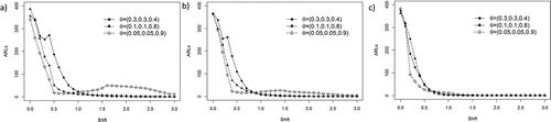
Figure 5 illustrates an ARL comparison for various and at different numbers of variable characteristics as summarized in Table 6. Figure 5 shows that the proposed chart has better performance in monitoring the process with extreme imbalanced parameters for small shifts in the process. However, it exhibits poorer performance in detecting large shifts in the process. On the other hand, for a process with balanced parameters, the proposed chart has better performance in detecting a large shift.

Figure 5. ARLs Comparison with several parameter of attribute characteristics for: a) p = 5 k = 4, b) p = 10 k = 6, c) p = 30 k = 15.

4. Application

4.1. Application to simulated process

In this section, the application of the proposed control chart is illustrated using the simulation data for several combinations of p, k, and parameters of attribute characteristics as summarized in Table 7. For this study, an in-control process with 70 observations for variable characteristics is assumed to follow a multivariate normal distribution , and the attribute characteristic follows a multinomial distribution The next 30 observations are the shifted process generated by multivariate normal distribution for variable characteristics, with the same process for attribute characteristics. The control limits used in this section are taken from Table 2.

Figure 6a shows the application of the proposed chart for scenarios i, ii, and iii. For all parameters of the attribute characteristics, the chart quickly detects a shift at the 71st observation. When the parameter of the attribute characteristic is extremely imbalanced for (scenario iii), the shifted process is not seen as clearly as with the other settings.

Figure 6. Application of control chart with simulation data.

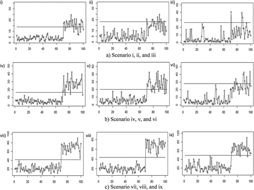
Figure 6b shows the application of the proposed chart for scenarios iv, v, and vi. Similar to the previous scenario, the chart quickly detects the shift at the 71st observation for all attribute characteristic parameters. Meanwhile, for an extreme imbalanced parameter of the attribute characteristic (scenario vi), it can be seen that the process is shifted, which is not clearly seen in the previous figure (scenario iii). Better results are found for scenarios vii, viii, and ix, as shown in Figure 6c. For all parameters of attribute characteristics, the proposed chart can clearly identify the shifts in the process. This is indicated by the fact that almost all of the shifted observations fall outside the control limit.

4.2. Application to a real case

In this section, the proposed chart is applied to a real case. The dataset used to evaluate the performance of the proposed chart is the Machine Failure dataset. This dataset can be downloaded at https://bigml.com/user/czuriaga/gallery/dataset/587d062d49c4a16936000810. The dataset is collected by monitoring a one-year basis machine, and the information about failures of the process is recorded. This dataset consists of 16 variable characteristics and three attribute characteristics.

The number of variable characteristics used in this study is eight, while the number of attribute characteristics is two. The number of principal components and the level of significance are five and 0.00273, respectively. The first 400 samples are treated as in-control observations (training dataset) and are used to estimate the control limit using KDE. By contrast, the 401st to 650th observations are treated as testing datasets and are monitored using the estimated control limit obtained from in-control observations.

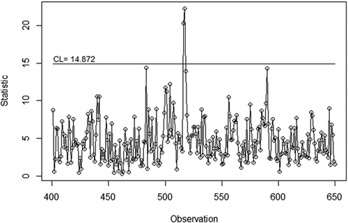
Figure 7 shows the utilization of the control chart to monitor the process for the testing dataset. The control limit obtained from KDE is 14.872. The original dataset has information about in-control and out-of-control labels for each observation so that the performance of the proposed control chart can be easily evaluated. Table 8 shows a performance comparison between the proposed chart and conventional chart in monitoring the real case. Given the null hypothesis that the observations in the testing dataset are in control, the proposed control chart produces zero false alarms and has an accuracy detection of about 99.6%. The proposed control chart successfully detects two of three actual out-of-control observations.

Table 8. Performance comparison between the proposed chart and conventional T² chart to monitor testing dataset in Machine Failure data.

Criteria	Number of observation
	Proposed Chart	Conventional
In-control observations	247	247
Out of control observations	3	3
Success detection of in-control observations	247	247
Success detection of out-of-control observations	2	1
Misdetection of in-control observations	0	0
Misdetection of out-of-control observations	1	2

Figure 7. Application of control chart to monitor the 401st to 650th observation of machine failure dataset using KDE control limit.

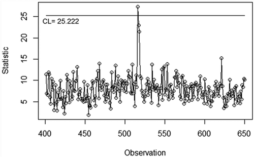
Compared to the proposed chart, the application of the conventional chart to monitor the process for the testing dataset is presented in Figure 8. Using the conventional F control limit (25.222), the conventional chart successfully detects the actual in-control and out-of-control observations with an accuracy of 99.2% and a detection rate of about 33.3% (detecting 1 out of 3 actual out-of-control observations). As a note, the number of actual out-of-control observations in the testing dataset is only three. These findings show that the proposed chart has better performance than the conventional chart when monitoring actual out-of-control observations.

Figure 8. Application of conventional control chart to monitor the 401st to 650th observation of Machine Failure dataset.

There are two reasons that the proposed chart has better performance. First, the proportion of the attribute characteristics of the testing dataset is balanced. The first attribute characteristic has eight categories with slightly balanced proportion (0.104, 0.223, 0.096, 0.100, 0.096, 0.127, 0.127, and 0.127), while the second attribute characteristic (four categories) has a balanced proportion (0.267, 0.259, 0.239, and 0.235). According to the simulation studies, for a small number of variable characteristics, the proposed chart is at the peak of its performance when it is used to monitor the balanced attribute characteristics (see Table 3 and Figure 6a). These facts reveal that a more accurate monitoring process will be achieved if these attribute characteristics are included in the analysis.

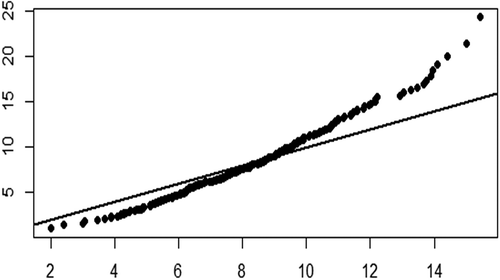
Second, the KDE control limit captures the actual out-of-control observations better than the conventional F distribution control limit, which was developed under a multivariate normal assumption. However, the eight variable characteristics in the Machine Failure testing dataset do not follow the multivariate normal distribution confirmed by the small p-value of the Mardiah test and the Q-Q plot, as shown in Figure 9. These facts indicate that the conventional control chart only has the best performance when an assumption is fulfilled. By using the KDE method, the empirical density of the statistic can be calculated, and the control limit can be estimated by taking its th percentile as defined in equation . The estimated KDE control limit is superior in detecting the actual out-of-control observations, whereas the conventional control limit is not.

Figure 9. The Q-Q plot of eight variable characteristics on Machine Failure testing dataset.

5. Managerial implication

In this globalization era, monitoring the quality of products using a control chart is essential for continuous process improvement. The main objective of a control chart is to monitor the process and reduce variations in the process. This monitoring process is done by identifying and eliminating assignable causes. An out-of-control observation issued by a control chart indicates the presence of assignable causes. To solve this problem, a root-cause analysis is conducted to reveal the reasons for the assignable causes. However, the conventional monitoring process using a control chart only considers one type of quality characteristic. For example, a variable control chart will be employed to monitor only numerical measurements such as weight and height, while an attribute control chart monitors categorical data such as the type of defect, color, and taste.

The findings in this study align with the concept of continuous improvement and the adaptive monitoring process with a mixed monitoring scheme using the proposed chart. This mixed scheme involves not only one type of quality characteristic but also both types of quality characteristic. Through simulation studies and application to a real case, this scheme was proven effective in monitoring shifts in the process. The decision-maker in a company can take fast corrective actions for any assignable causes that occur owing to the sensitivity of the proposed scheme. Furthermore, the in-control observations obtained from past monitoring processes need to be stored in a database in order to improve the production process in the future.

Along with the development of the company, the production capability and level of accuracy of the production machinery will increase. As an implication of this development, the monitoring control limit needs to be adjusted. Using the KDE method, the historical in-control data production is used to generate new control limits by fitting its statistical distributions. This new adjusted control limit will help the company to improve its production quality with stricter criteria for in-control products. Thus, this monitoring scheme guarantees precision and accuracy in monitoring the manufacturing process, and ensures the adaptability of the monitoring system to evolve continuously with developments in science and technology.

6. Conclusions

In this paper, a new control chart to monitor a process with variable and attribute characteristics is presented using the PCA Mix concept. Simulation studies showed that for several combinations of number of quality characteristics, number of PCs, and values of multinomial parameters, the control limit using the KDE method always results in an ARL₀ at about 370 for . Meanwhile, the ARL₀ of the control chart using a conventional control limit is not stable. For the shifted process, the ARL₁ of the proposed chart is quickly decreased as the shift from both variable and attribute characteristics increases. The control chart has better performance when it uses an appropriate number of principal components. Moreover, the applications for simulation data and real cases also show that the proposed chart is sensitive to monitoring the shifted process. The present work can be extended to learn how the mixed process with both variable and attribute characteristics affects the monitoring system not only in industries and services but also in other fields such as healthcare and network security systems. This study will also trigger the development of multivariate mixed charts for non-normal distribution. In addition, the bootstrap resampling method can be considered to replace the KDE for control limit estimation.

Disclosure statement

No potential conflict of interest was reported by the authors.

Additional information

Funding

This work was supported by Research, Technology, and Higher Education Ministry, the Republic of Indonesia through PMDSU scheme under Grant [128/SP2H/PTNBH/DRPM/2018].

References

- Abu‐Shawiesh, M. O. A., Kibria, G., & George, F. (2014). A robust bivariate control chart alternative to the hotelling’s T2 control chart. Quality and Reliability Engineering International, 30(1), 25–35.
- Ahsan, M., Mashuri, M., & Khusna, H. (2018). Intrusion detection system using bootstrap resampling approach of T2 control chart based on successive difference covariance matrix. Journal of Theoretical and Applied Information Technology, 96(8), 2128-2138.
- Ahsan, M., Mashuri, M., Kuswanto, H., Prastyo, D. D., & Khusna, H. (2018). T 2 control chart based on successive difference covariance matrix for intrusion detection system. Journal of Physics: Conference Series, 1028, 12220. IOP Publishing.
- Alfaro, J. L., & Ortega, J. F. (2009). A comparison of robust alternatives to Hotelling’s T2 control chart. Journal of Applied Statistics, 36(12), 1385–1396.
- Ali, H., Syed Yahaya, S. S., & Omar, Z. (2013). Mathematical problems in engineering. Robust Hotelling T2 Control Chart with Consistent Minimum Vector Variance, 2013. doi:10.1155/2013/401350
- Alkindi, Mashuri, M., & Prastyo, D. D. (2016). T2 hotelling fuzzy and W2 control chart with application to wheat flour production process. AIP Conference Proceedings, 1746. doi:10.1063/1.4953977
- Amdouni, A., Castagliola, P., Taleb, H., & Celano, G. (2017). A variable sampling interval Shewhart control chart for monitoring the coefficient of variation in short production runs. International Journal of Production Research, 55(19), 5521–5536.
- Arkat, J., Niaki, S. T. A., & Abbasi, B. (2007). Artificial neural networks in applying MCUSUM residuals charts for AR(1) processes. Applied Mathematics and Computation, 189(2), 1889–1901.
- Aslam, M., Azam, M., Khan, N., & Jun, C. H. (2015). A mixed control chart to monitor the process. International Journal of Production Research, 53(15), 4684–4693.
- Aslam, M., Khan, N., Aldosari, M. S., & Jun, C. H. (2016). Mixed control charts using EWMA statistics. IEEE Access, 4, 8286–8293.
- Aslam, M., Srinivasa Rao, G., Ahmad, L., & Jun, C.-H. (2017). A control chart for multivariate Poisson distribution using repetitive sampling. Journal of Applied Statistics, 44(1). doi:10.1080/02664763.2016.1164837
- Bersimis, S., Psarakis, S., & Panaretos, J. (2007). Multivariate statistical process control charts: An overview. Quality and Reliability Engineering International. doi:10.1002/qre.829
- Bersimis, S., Sgora, A., & Psarakis, S. (2016). The application of multivariate statistical process monitoring in non-industrial processes. Quality Technology and Quantitative Management, 3703(September), 1–24.
- Burden, R. L., & Faires, J. D. (2011). Numerical Analysis. Cengage Learning.doi: 10.1017/CBO9781107415324.004
- Chavent, M., Kuentz-Simonet, V., Labenne, A., & Saracco, J. (2014). Multivariate analysis of mixed data: The PCAmixdata R package.
- Chen, G., Cheng, S. W., & Xie, H. (2005). A new multivariate control chart for monitoring both location and dispersion. Communications in Statistics—Simulation and Computation®, 34(1), 203–217.
- Chena, L. H., Chang, F. M., & Chen, Y. L. (2011). The application of multinomial control charts for inspection error. International Journal of Industrial Engineering : Theory Applications and Practice, 18(5), 244–253.
- Chiu, J. E., & Kuo, T. I. (2008). Attribute control chart for multivariate poisson distribution. Communications in Statistics - Theory and Methods, 37(1), 146–158.
- Chou, Y.-M., Mason, R., & Young, J. (2001). The control chart for individual observations from a multivariate non-normal distribution. Communications in Statistics: Theory & Methods, 30(8/9), 1937.
- Cozzucoli, P. C. (2009). Process monitoring with multivariate p-control chart. International Journal of Quality, Statistics, and Reliability, 2009, 1–11.
- De Leeuw, J., & Van Rijckevorsel, J. (1980). HOMALS and PRINCALS—Some generalizations of principal components analysis. Data Analysis and Informatics, 2, 231–242.
- Gunaratne, N. G. T., Abdollahian, M. A., Huda, S., & Yearwood, J. (2017). Exponentially weighted control charts to monitor multivariate process variability for high dimensions. International Journal of Production Research, 55(17), 4948–4962.
- Issam, B. K., & Mohamed, L. (2008). Support vector regression based residual MCUSUM control chart for autocorrelated process. Applied Mathematics and Computation, 201(1–2), 565–574.
- Jolliffe, I. T. (2002). Principal component analysis. Journal of the American Statistical Association, 98, 487.
- Khan, N., Aslam, M., Kim, K.-J., & Jun, C.-H. (2017). A mixed control chart adapted to the truncated life test based on the Weibull distribution. Operations Research and Decisions, 27(1), 43–55.
- Khusna, H., Mashuri, M., Suhartono, S., Prastyo, D. D., & Ahsan, M. (2018). Multioutput least square SVR based multivariate EWMA control chart. Journal of Physics: Conference Series, 1028(1), 12221. Retrieved from http://stacks.iop.org/1742-6596/1028/i=1/a=012221
- Kiers, H. A. L. (1988). Principal components analysis on a mixture of quantitative and qualitative data based on generalized correlation coefficients. The Many Faces of Multivariate Analysis, 1, 67–81.
- Kiers, H. A. L. (1989). Three-way methods for the analysis of qualitative and quantitative two-way data. Leiden: DSWO press Leiden.
- Kiers, H. A. L. (1991). Simple structure in component analysis techniques for mixtures of qualitative and quantitative variables. Psychometrika, 56(2), 197–212.
- Kim, D., & Lee, I.-B. (2003). Process monitoring based on probabilistic PCA. Chemometrics and Intelligent Laboratory Systems, 67(2), 109–123.
- Kourti, T. (2005). Application of latent variable methods to process control and multivariate statistical process control in industry. International Journal of Adaptive Control and Signal Processing, 19(4), 213–246.
- Laungrungrong, B. (2010). Multivariate charts for multivariate Poisson-distributed data. Arizona: Arizona State University.
- Lowry, C. A., & Montgomery, D. C. (1995). A review of multivariate control charts. IIE Transactions (Institute of Industrial Engineers), 27(6), 800–810.
- Montgomery, D. (2009). Introduction to statistical quality control. New York: John Wiley & Sons Inc. doi:10.1002/1521-3773(20010316)40:6<9823::AID-ANIE9823>3.3.CO;2-C
- Mukhopadhyay, A. R. (2008). Multivariate attribute control chart using Mahalanobis D2 statistic. Journal of Applied Statistics, 35(4), 421–429.
- Niaki, S. T. A., & Abbasi, B. (2007a). Skewness reduction approach in multi-attribute process monitoring. Communications in Statistics - Theory and Methods, 36(12), 2313–2325.
- Niaki, S. T. A., & Abbasi, B. (2007b). On the monitoring of multi-attributes high-quality production processes. Metrika, 66(3), 373–388.
- Niaki, S. T. A., & Khedmati, M. (2013). Estimating the change point of the parameter vector of multivariate Poisson processes monitored by a multi-attribute T 2 control chart. International Journal of Advanced Manufacturing Technology, 64(9–12), 1625–1642.
- Noorossana, R., & Vaghefi, S. J. M. (2006). Effect of autocorrelation on performance of the MCUSUM control chart. Quality and Reliability Engineering International, 22(2), 191–197.
- Parzen, E. (1962). On estimation of a probability density function and mode. The Annals of Mathematical Statistics, 33(3), 1065–1076.
- Phaladiganon, P., Kim, S. B., Chen, V. C. P., Baek, J.-G., & Park, S.-K. (2011). Bootstrap-based T 2 multivariate control charts. Communications in Statistics - Simulation and Computation, 40(5), 645–662.
- Phaladiganon, P., Kim, S. B., Chen, V. C. P., & Jiang, W. (2013). Principal component analysis-based control charts for multivariate nonnormal distributions. Expert Systems with Applications, 40(8), 3044–3054.
- Pirhooshyaran, M., & Niaki, S. T. A. (2015). A double-max MEWMA scheme for simultaneous monitoring and fault isolation of multivariate multistage auto-correlated processes based on novel reduced-dimension statistics. Journal of Process Control, 29, 11–22.
- Pu, X., Li, Y., & Xiang, D. (2011). Mixed variables-attributes test plans for single and double acceptance sampling under exponential distribution. Mathematical Problems in Engineering, 2011. doi:10.1155/2011/575036
- Rosenblatt, M. (1956). Remarks on some nonparametric estimates of a density function. The Annals of Mathematical Statistics, Volume, 27, 832–837.
- Seif, A., Faraz, A., Saniga, E., & Heuchenne, C. (2016). A statistically adaptive sampling policy to the Hotelling’s T2 control chart: Markov chain approach. Communications in Statistics - Theory and Methods, 45(13), 3919–3929.
- Sorooshian, S. (2013). Basic developments of quality characteristics monitoring. Journal of Applied Mathematics, 2013, 1–8.
- Umit, F., & Cigdem, A. (2001). Multivariate quality control: A historical perspective. Yilditz Technical University, 54–67. doi:10.1016/S0168-6496(03)00201-0
- Wibawati, M., Purhadi, M., & Irhamah. (2016). Fuzzy multinomial control chart and its application. AIP Conference Proceedings, 1718. doi:10.1063/1.4943351
- Wibawati, Mashuri, M., Purhadi, Irhamah & Ahsan, M. (2018). Performance fuzzy multinomial control chart. Journal of Physics: Conference Series, 1028(1), 12120. Retrieved from http://stacks.iop.org/1742-6596/1028/i=1/a=012120