Batch process control and monitoring: a Dual STATIS and Parallel Coordinates (DS-PC) approach

ABSTRACT

Multivariate data collected from batches is usually monitored via control charts (CCs) based on MPCA and MPLS for batch to batch comparison. In addition, distribution free approaches include other dimensionality reduction methods for batch and time-wise analysis. However, techniques for multivariate data focused on variable-wise analysis haven’t been widely developed. Here, we propose a nonparametric quality control strategy for off-line monitoring of batches and variables, besides visual clustering of observations within batches. In our approach, CCs based on Dual STATIS are created using robust bagplots to enhance signal detection in batch and variable-wise analysis, while parallel coordinate plots are used in identification of unusual observations’ behavior per variable, regardless distributional assumptions. This proposed strategy poses the main advantage of detecting different type of changes through meaningful visualization tools, allowing easier interpretation of results in industrial settings.

KEYWORDS:

• Batch process
• off-line monitoring
• Dual STATIS
• Parallel Coordinates
• multivariate control charts

1. Introduction

Nowadays, several industries rely on batch processing, including for example, chemicals, pharmaceuticals, food products, fabrics, metals, bakeries, pulp, and paper manufacturers. The batch is the primary processing unit in which raw materials are loaded into and then a series of transformations take place to yield final products. High-quality products are commonly described by quality characteristics (variables), each of which must be controlled within specifications to maintain customer satisfaction and to describe the process performance as the batch progresses (Lewis, 2014; Niang, Fogliatto, & Saporta, 2013).

Statistical process control (SPC) for monitoring industrial processes always involves simultaneous monitoring or control of two or more correlated quality-process characteristics. In this sense, multivariate control charts (CCs) replace the univariate ones, usually applied in monitoring, because analyzing these characteristics under the univariate case can be misleading (Montgomery, 2009). Results obtained from multivariate CCs are strongly recommended when quality characteristics are correlated (Bersimis, Psarakis, & Panaretos, 2007). The most frequently used multivariate CC is the Hotelling or T² chart (Hotelling, 1947). Other multivariate CCs are presented and reviewed by Jackson (1991); Wierda (1994); Lowry and Montgomery (1995) and Harris, Seppala, and Desborough (1999).

Assumptions of independence and multinormality are not always verifiable in practice, leaving traditional multivariate CCs unusable. CCs based on bootstrap methods (Liu & Tang, 1996) and nonparametric CCs (Liu, 1995; Lombardo, Vanacore, & Durand, 2008) should be considered to overcome the limitations in case of dependent measurements or nonnormal data. In addition, traditional multivariate CCs are not efficient when variables’ nominal behaviors are described by profiles as for data arising from batch processes, which are likely to display a strong correlation-autocorrelation structure (Niang et al., 2013).

Monitoring batch processes through multivariate CCs was first described by Jackson and Mudholkar (1979), and later investigated by Kourti, Nomikos, and MacGregor (1995), Nomikos and MacGregor (1995), Kourti and MacGregor (1996), and Macgregor (1997). Applications of those CCs in batch processes may be found in Flores-Cerrillo and MacGregor (2002), among others, considering multinormality assumptions.

The principal contributions in the literature came with multivariate projection methods, which reduce high dimensional data into low-dimensional ‘latent variables’. Statistical projection methods, such as principal component analysis (PCA) and partial least squares (PLS) ideally provide, at some degree of confidence, a representation of the correlation structure within data (Lewis, 2014). As for our concern, approaches to batch monitoring are mostly grounded on multiway partial least squares (MPLS) and multiway principal component analysis (MPCA) (Filho & Luna, 2015; Kourti, 2003). Additional issues of the multivariate version refer to its limitation with dynamic variables’ behavior of batch processes and real-time monitoring of ongoing batches (Filho & Luna, 2015).

An alternative way of monitoring batch processes was provided by STATIS. Its pioneer use in quality control was orientated toward off-line monitoring (Scepi, 2002). In recent contributions, STATIS has been used in off-line and on-line monitoring taking into account the use of IS and CO CCs for batches of fixed time duration and its dual version for variable duration (Filho & Luna, 2015; Fogliatto & Niang, 2009; Niang et al., 2013; Niang, Fogliatto, & Saporta, 2009). These STATIS-based approaches have carried out batch and time-wise analysis, including bivariate boxplots, based on convex hull peeling and B-spline smoothing for CCs’ construction, under nonparametric conditions. However, none complementary analysis was conducted to examine behavior within batches per variable (Filho & Luna, 2015; Fogliatto & Niang, 2009; Niang et al., 2009).

Even though parallel coordinate plotting is a well-recognized visualization technique, it was not until 2004, where its successful implementation for monitoring data variability in several industrial facilities, led to its versatile application in multivariate SPC (Lange, Rodriguez, Puech, & Vasques, 2011; Wang, Medasani, Marhoon, & Albazzaz, 2004). Additionally, parallel coordinate plots have been used to categorize data into normal and abnormal operating conditions in hazard identification (Comfort, Warner, Vargo, & Bass, 2011). Its latest contribution in process monitoring was presented in combination with PCA technique, which delivers visualization of confidence regions, evaluation of models with different number of principal components, comparison of faulty events, and determination of false alarms’ frequency in actual process data (Dunia, Edgar, & Nixon, 2012).

In this paper, we propose a nonparametric quality control strategy based on IS and CO CCs which enables off-line monitoring of batch processes using Dual STATIS and bagplots for establishing control regions. A complementary analysis is developed with parallel coordinate plotting to examine tendencies within out-of-control batches. Our work extends recent approaches where the use of the STATIS method has focused on time-wise analysis. In this sense, our combined strategy brings on a variable-wise analysis, leading to support the visual interpretation of out-of-control signals. Then, industries will be able to determine if quality specifications are met, resulting in cost and time savings.

The remaining sections are organized as follows. A brief review of STATIS, Dual STATIS and Parallel Coordinates is provided in Sections 2.1 and 2.2. The proposed DS-PC strategy is detailed in Section 2.3. Application of the strategy on two case studies is described in Sections 3.1 and 3.2. Finally, discussion and conclusions are delivered in Sections 4 and 5.

2. Methodology

2.1. STATIS & Dual STATIS

STATIS, an acronym which stands for the French expression ‘Structuration des Tableaux À Trois Indices de la Statistique’, was initially proposed by L'Hermier des Plantes (1976) and later described by Escoufier (1987) and Lavit, Escoufier, Sabatier, and Traissac (1994). This multivariate data analysis method is aimed at exploring and analyzing the structure of several data tables obtained under different scenarios. The multiple data tables are sets of variables’ measurements on the same observations. The method reduces the dimensionality of three-way data arrays through a similarity measure based on Euclidean distances between points’ configurations. A recent review on this method and its extensions is available in Abdi, Williams, Valentin, and Bennani-Dosse (2012).

In opposition to STATIS, Dual STATIS works in such way that individuals vary from one scenario to another, remaining the same variables. Dimensionality reduction performed via EVD, SVD and GSVD, allows for the visualization of the salient features of tables and variables. Data consist of sets of observations (tables) measured on the same set of variables. Here, instead of computing cross-product matrices between the observations, we compute covariance matrices between the variables (one per set of observations). Then, Dual STATIS approach follows the same steps as standard STATIS and will provide a compromise map for the variables (instead of the observations) (Abdi et al., 2012).

Zero step: tables preprocessing

Dual STATIS method considers tables including observations (individuals) and variables; each one of these represents different studies, scenarios or batches. Raw tables must be preprocessed using several methods of centering, scaling, and normalizing data as shown in Tucker (1964), Westerhuis, Kourti, and MacGregor (1998), Næs, Brockhoff, and Tomic (2010), Abdi et al. (2012) and Filho and Luna (2015).

Centering, scaling, and normalizing are typically based on per-table statistics. Nonetheless, for quality control purposes, centering and scaling are performed with the global mean and standard deviation of the variables for all tables, thus capturing the under-control behavior. This is possible because all variables are shared among the tables. Since the tables have different number of rows, they are normalized dividing each table by its number of rows.

First step: interstructure analysis

In this way, preprocessed matrices with dimension can be obtained. These matrices are vertically stacked to structure the matrix with rows and columns, where . exhibits horizontal partitioning which makes sense for Dual STATIS cases. For each table, a cross-product matrix is obtained:

(1)

Each cross-product symmetric matrix is vectorized (converted in a vector by placing its rows one after another). Then, the obtained vectors are stored in a new matrix of dimension .

The Interstructure matrix of dimension is computed from the matrix product . This positive semidefinite matrix allows representing in two dimensions each one of tables using Eigenvalue Decomposition (EVD), considering that eigenvalues are sorted from the largest to the smallest:

(2)

where is a matrix containing the eigenvectors of and is a diagonal matrix which collects the corresponding eigenvalues.

An optional way for computing is performing a Singular Value Decomposition (SVD) of the matrix :

(3)

Let be the rank of the matrix , is a matrix containing the left singular vectors of , a diagonal matrix which collects the singular values of , and stores the right singular vectors of in a matrix.

EVD of allows to represent tables as points in a two-dimensional PCA map called Interstructure Space (IS), using first and second columns of the matrix as coordinates:

(4)

This particular representation, also called biplot, was first introduced by Gabriel (1971) and later modified by Galindo (1986). A biplot allows information on both individuals and variables of a data matrix to be displayed graphically. The IS CC is based on this plot.

A new preprocessed table can be projected onto the interstructure space by computing a supplementary cross-product matrix , vectorizing it, and generating the correspondent matrix of dimension . Then, the associated point in the interstructure space is determined using first and second columns of the matrix as coordinates:

(5)

From the interstructure space, an optimal set of weights for the tables is derived to compute the best common representation of the variables (Abdi et al., 2012). These weights are determined by rescaling the first eigenvector of and dividing it by the sum of its elements, defining the vector as:

(6)

Then, the optimum weights’ diagonal matrix is computed as follows. The values from are stacked and each value is repeated times according to the number of observations in each table. Note that is a square matrix of order .

Second step: intrastructure analysis

A mass, denoted , is assigned to each variable. Masses are nonnegative elements whose sum equals one. Although different masses can be computed for each variable, often equal masses are chosen to assure that all variables have the same importance for analysis (Abdi et al., 2012).

A diagonal matrix for variables’ masses is obtained dividing the identity matrix by the number of variables :

(7)

Now the triplet is conformed by preprocessed tables, weights, and masses.

Using the general singular value decomposition (GSVD) of the triplet, the following decomposition is computed:

(8)

Let be the rank of the matrix , is a matrix containing the left singular vectors of , a diagonal matrix which collects its singular values, and stores the right singular vectors in a matrix.

This decomposition will provide a Compromise Space for the representation of variables into a reduced dimension map, which constitutes the basis for CO CCs.

Compromise Factor Scores allow plotting variables into the compromise map. These scores are computed as the first and second columns of the matrix:

(9)

Recall that partial factor scores can be defined as the projection of -th table onto its left singular vectors (Abdi et al., 2012). Then, the partial factor scores for this table are computed as the first and second columns of the matrix:

(10)

As suggested in Equation 9, the compromise factor scores matrix is also the weighted average of the partial factor scores and is considered as the barycenter (Abdi et al., 2012).

Therefore, for computing the partial factor scores, matrix is horizontally partitioned in matrices of dimension denoted with the same number of rows that . Matrix is calculated from Equation 8 as described:

(11)

Variables of a new preprocessed table can be projected onto the compromise space by obtaining the following matrices:

(12)

Then, the associated points in the compromise space are determined using first and second columns of the matrix as coordinates. In CO CCs, these points are compared against the partial factor scores of the tables to detect out-of-control cases.

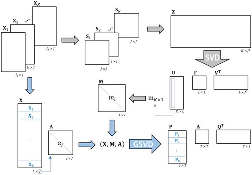
Dual STATIS steps are summarized in the scheme shown in Figure 1.

Figure 1. Dual STATIS representation including interstructure and intrastructure analysis: The first step also known as interstructure analysis is represented by gray arrows while the second step, commonly referred as intrastructure analysis is represented by light blue arrows. Zero step is not shown.

2.2. Parallel Coordinates

Parallel Coordinates as a graphical representation system was proposed by Alfred Inselberg from which -dimensions could be represented in a two-dimensional system (Inselberg & Dimsdale, 1990). As Dual STATIS, parallel coordinate plotting is used to display multi-dimensional data in two dimensions in order to identify homogeneous patterns of data among many different variables (Heinrich & Weiskopf, 2013). When lines present a similar behavior, this tool is very useful in identifying clusters between observations (Inselberg, 2009). In this sense, Parallel Coordinates can be used for ‘visual clustering’, i.e. to find groups of similar points based on visual features such as the proximity of lines or line density (Heinrich & Weiskopf, 2013). For control and monitoring, Parallel Coordinates capacity for clustering and summarization are of great importance in plotting confidence regions (Dunia et al., 2012).

Each observation within tables is represented in dimensions or variables by a polygonal of sides. In addition, the correlation analysis between variables focuses on intersections from polygonals that are constructed from raw tables (Inselberg, 2009; Wegman, 1990).

2.3. DS-PC strategy

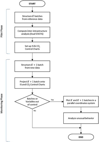
DS-PC strategy stands for the combination of Dual STATIS and Parallel Coordinates. The proposal (Figure 2) is based on nonparametric CCs provided by DS and plots in two-dimensional system derived from PC.

Figure 2. Overall view of DS-PC strategy: DS-PC strategy proposed for off-line control is presented in two phases, pilot and monitoring. Pilot phase refers to setting up IS and CO_j control charts based on reference data. Monitoring phase focuses in the new batch projection onto the CCs previously established and gathers information of its performance through Parallel Coordinates.

During the pilot phase, the data set must be preprocessed to structure reference batches, as described previously on zero step. This preprocessing is vital for the later detection of out-of-control signals. Afterwards, Dual STATIS analyses are computed to obtain the interstructure matrix , the compromise matrix , and the partial factor scores matrix per batch. This information is crucial for setting up IS and CO_j CCs.

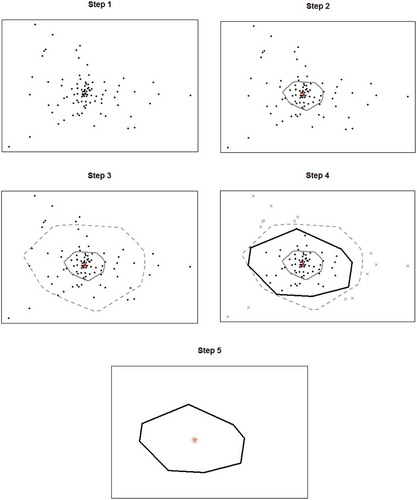
The charting procedure begins with the construction of control regions, which are based on bagplots (Rousseeuw, Ruts, & Tukey, 1999). The bagplot represents a bivariate generalization of the univariate boxplot in which ‘depth median’ plays the role of the robust centroid and it is surrounded by a convex polygon that defines the control region for the referred charts (Figure 3).

Figure 3. Setting up in-control region: Five steps are needed to generate the control region from data points through bagplots.

Input information for control regions is provided by matrices and , calculated from in-control batches. The two first columns of matrix represent batches’ position in the interstructure space (IS) and the two first columns of matrix exhibit the coordinates of each batch per variable (defined by its corresponding row) into the compromise space (CO_j).

The initial step, for building up control regions, consists in plotting input information as data points. Now, the median (symbolized with *) is calculated from the sketched data points and a bag containing 50% of these data points is plotted. Then, bag’s magnification by a factor of three yields the fence, which separates in-control and out-of-control states (outliers) (Gower, Gardner-Lubbe, & le Roux, 2011). This factor ensures that 99.8% of the data is included in the control region giving a probability of desired false alarms, under normality assumption (Zani, Riani, & Corbellini, 1998). The fence determines the control region performed directly on principal plane displays obtained using Dual STATIS. Finally, the fence is not considered as part of the bagplot, hence data points that are not marked as outliers are surrounded by a loop, the convex polygon of the observations within the fence (Narayanachar, 2013; Rousseeuw et al., 1999). This algorithm is illustrated in Figure 3.

These control regions test our bivariate statistics calculated for new structured tables during the monitoring phase from new batches, leading to IS and CO_j CCs. Each table is then projected onto interstructure and compromise spaces through matrices and .

Off-line control of a new batch starts with the projection of the corresponding data matrix into IS CC using Equations (1) and (5). It is important to remark that information of the new batch will be entirely available and has already been preprocessed. In addition, new batch’s projection into CO_j CC is done using Equation (12). At the same time, parallel coordinate plotting is done with the information of several reference batches and the new one to distinguish any abnormal performance on variables’ axes.

According to DS-PC strategy, new batches can be signaled as out-of-control or in-control. Figures 4 and 5 portray self-explanatory cases in IS and CO_j CCs, whereas Figure 6 exemplifies both cases in parallel coordinate plots.

Figure 4. IS control chart: The loop determines the IS control region and the red asterisk within the region represents the robust centroid. Blue point represents a batch out of control (BO). Black point represents a batch in control (BI).

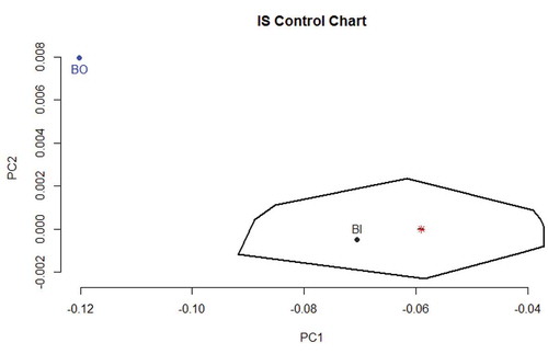
Figure 5. CO_j control charts: CO_j control regions and their respective asterisks are plotted for a trivariate case. Blue points indicate an out-of-control batch (BO) for correspondent variables 1, 2 and 3. Black points are indicatives of an in-control batch (BI) for the three variables.

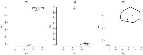
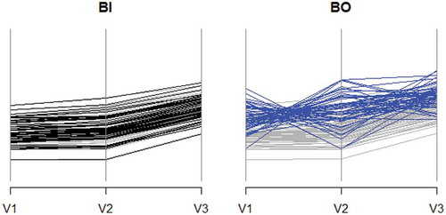
Figure 6. Parallel coordinate plots: Parallel coordinate system is set with variables’ axes equally scaled. Each observation is plotted as a polygonal. Observations within reference behavior are plotted in gray. Black and blue ones represent new observations coming from batches (BI) and (BO). As expected, black polygonals correspond to a batch in control (BI). However, blue polygonals clearly show an unusual behavior within batch (BO).

3. Case studies

To evaluate the performance of the proposed strategy, two case studies are developed in this section. The first one is an illustrative example that simulates a batch process. The second one is the fed-batch penicillin fermentation process, a well-known benchmark batch process. All simulations and analyses were computed in open source software R.

3.1. Illustrative example

In plastic bags fabrication industry, data of 200 reference batches () were simulated. For each batch, three process variables () and 50 individuals () were recorded. The means and standard deviations were chosen from expected standards, and the correlation matrix was proposed by the authors to represent normal behavior of process. These values are shown in Table 1.

Table 1. Reference batches information for the illustrative example.

Mean Vector
Standard Deviation Vector
Correlation Matrix

The correlated structure of the data was introduced through Cholesky decomposition of variance and covariance matrix (Golub & Van Loan, 1996; Horn & Johnson, 2013; Trefethen & Bau, 1997). In this sense, the reference data set was formed by random batches that follow a multivariate normal distribution.

Additionally, a set of eight batches was simulated to exemplify the performance of the DS-PC strategy indicated in Section 2.3. This set consisted of one good batch (in control) and seven bad batches (out of control). Variables were perturbed to simulate bad batches according to mean, standard deviation, and correlation shifts, shown in Table 2. Some batches introduced individual shifts and others exhibited a combination of different shifts.

Table 2. Tested batches for the illustrative example.

Batches
Mean Shifts	None	✓	None	None	✓	None	✓	✓
Standard Deviation Shifts	None	None	✓	None	✓	✓	None	✓
Correlation Shifts	None	None	None	✓	None	✓	✓	✓

After analyzing the 200 reference data sets and 8 training batches using Dual STATIS method, graphical representations of interstructure and compromise behavior were obtained.

IS CC shows training batches’ projection in Figure 7. As expected, batch falls within the control region while remaining batches from to are signaled to be out of control.

Figure 7. IS and CO_j control charts for the illustrative example: Points in black correspond to batches without shifts. The color used for batches exhibiting different levels of shifts is blue. The IS and CO_j CCs were plotted with 7 batches signaled as out of control.

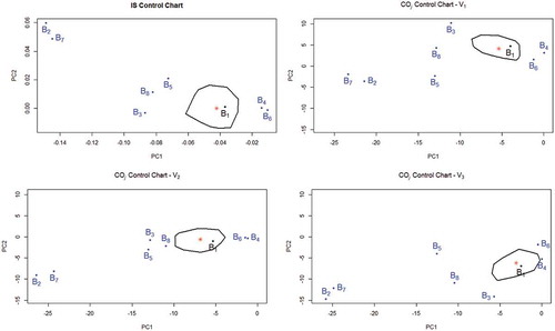
The next step in our strategy is to plot CO_j CCs to investigate which variables are responsible for the signals. To facilitate the analysis, a graph, equally scaled, has been plotted for each variable as shown in Figure 7. CO_j CCs signal the three variables in an out-of-control state.

Bad batches show anomalous behavior within the three variables analyzed. However, this visual aid doesn’t allow to examine the types of shifts that batches suffered. Complementary analysis carried out with Parallel Coordinates is shown in Figure 8. This technique allows comparison in terms of observations’ tendencies from several reference batches and the ones derived from the batches out of control.

Figure 8. Parallel coordinate plots for the illustrative example: Observations within reference behavior are plotted in gray and the ones in blue represent new observations coming from ongoing batches during the process. Batch represents no shifts; remaining batches portray mean, standard deviation, correlation shifts, and shifts’ combination in three variables.

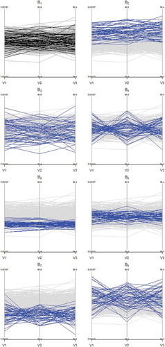
Batch presents a normal pattern within boundaries defined by reference batches. However, exhibits values above the mean, which evidences an increase for the three variables tested. shows confidently standard deviation shifts with values falling out of the reference pattern. Although, almost linear positive correlation between variables is presented in , intersection points between polygonals demonstrate a linear negative correlation in batch , reflecting greater changes in correlation structure. Batch exhibits changes for the three variables because of values under the mean and with smaller deviation than usual. also presents values with less deviation than the normal pattern and an unnoticeable decrease in correlation coefficients that presents a limitation for its visualization due to combined situations. Batch has values under the mean and evidences moderate changes in correlation due to a negative factor, yet this shift is not easily detected. Finally, presents three types of shifts, values above the mean, greater standard deviations, and change of sign in correlation coefficients, being the last one more noticeable than in batch .

3.1.1. Simulations

As suggested by Filho and Luna (2015), for an overall examination of IS and CO_j CCs efficiency, 11 simulated scenarios with 10,000 runs each, were computed. Results are shown in Table 3.

Table 3. Simulation results of IS and CO_j control charts performance for the illustrative example.

Scenarios 10,000 runs per each	% out-of-control cases				Type of alarm
	IS CC	CO CC
		Variable 1	Variable 2	Variable 3
	5.30	6.49	5.92	4.96	FALSE
	93.52	97.41	88.00	96.08	TRUE
	100.00	100.00	99.99	100.00	TRUE
	70.25	30.48	41.03	21.78	TRUE
	98.60	91.09	93.66	90.55	TRUE
	13.06	13.67	17.87	4.39	TRUE
	94.41	80.84	93.70	15.94	TRUE
	97.17	86.49	91.45	85.05	TRUE
	30.91	28.25	24.49	35.40	TRUE
	79.83	94.81	65.90	93.41	TRUE
	100.00	100.00	100.00	100.00	TRUE

Scenario with no changes, presents a low percentage of false alarms in both charts. However, mean shifts of ±4% and ±6% evidence high percentage of signal detection in all perturbed variables. Standard deviation shifts of ±20% and ±40% in three variables, reveal greater detection in greater shifts. When the correlations are affected in a similar way, detection rate depends on the variation respect to the original correlation values, reflecting high percentage of detection, between more correlated variables, under significant change of correlation structure.

In general, combined shifts increase the percentage of out-of-control cases’ detection when mean shifts were involved due to high sensibility for detecting this type of changes. However, standard deviation and correlation associated shifts exhibit better detection than correlation shifts individually when maintaining coefficients’ sign. Finally, scenarios with the three types of shift produce better detection in comparison with those where two types of shift were introduced. Although performing efficiently in several scenarios as presented above, some aspects of STATIS-based CCs may require further refinements in the method and complementary analysis.

3.1.2. Power curves comparison

Hundred sequential factors were tested in performance simulations (1,000 runs per each) for evaluating different levels of proportional shifts for mean, standard deviation, and correlation coefficients in the IS CC. Figures 9–11 show the percentage of out-of-control cases vs. the factor for defining the mentioned shifts. The green line corresponds to the use of bagplot with depth median as robust centroid for setting up the control region and the red line to the use of convex hull peeling and B-spline smoothing developed in Niang et al. (2009).

Figure 9. Power curve for the mean: The -axis represents the percentage of out of control cases and the -axis represents a factor shift for the mean vector. The green line represents the values obtained when the control region setup involves the bagplot and the red line, when convex hull peeling and B-spline smoothing is used.

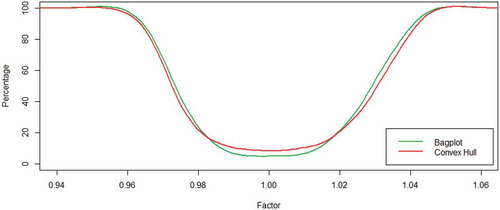
Figure 10. Power curve for the standard deviation: The -axis represents the percentage of out of control cases and the -axis represents a factor shift for the standard deviation vector. The green line represents the values obtained when the control region setup involves the bagplot and the red line, when convex hull peeling and B-spline smoothing is used.

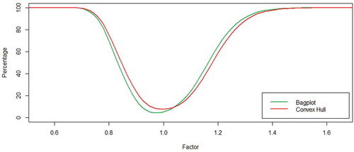
Figure 11. Power curve for the correlation coefficient: The -axis represents the percentage of out of control cases and the -axis represents a factor shift for the correlation coefficients. The green line represents the values obtained when the control region setup involves the bagplot and the red line, when convex hull peeling and B-spline smoothing is used.

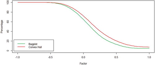
Figure 9 shows that bagplots classify good and bad batches better than convex hull, leading to smaller number of false alarms within ±1.5 % of mean shifts and total discard when shifts are higher than ±4%. Figure 10 evidences a slight asymmetry to the left, meaning bagplot performs better than convex hull detecting bigger dispersion rapidly. Although, any industrial process seeks for the smallest possible dispersion, detection of the opposite situation is significantly privileged. Factors less than 0.7 and more than 1.5 lead to a total discard of the batch in both cases. In Figure 11, a proportional correlation shift is not easily detected in bagplots; as is observed, convex hull performs better. However, they both have a total discard when coefficients shift in the negative direction is greater than 50% with a maximum shift of 100% (factor equals −1).

3.2. Fed-batch penicillin fermentation process

In this section, the fed-batch penicillin fermentation process is used as a practical application of DS-PC approach. This well-known benchmark simulation process is widely applied to evaluate the batch process monitoring and fault diagnosis methods (Albazzaz, 2004; Birol, Ündey, & Çinar, 2002; Doan & Srinivasan, 2008; Hanyuan & Xuemin, 2017; Lee, Yoo, & Lee, 2004; Yoo, Lee, Vanrolleghem, & Lee, 2004). Its flow diagram is shown in Figure 12.

Figure 12. Diagram flow of the fed-batch penicillin fermentation process: The diagram shows the physical system for the process as appeared in the PenSim v1.0, Illinois Institute of Technology.

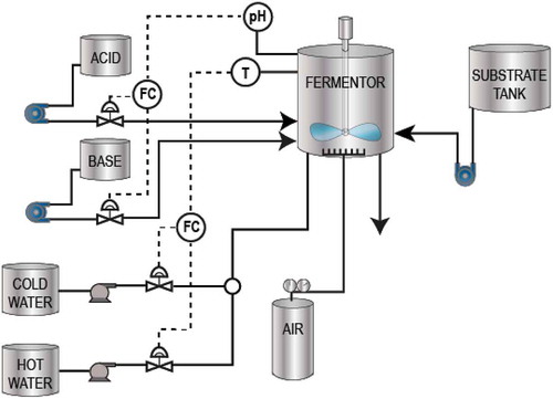
This process involves two operation stages including the preculture stage and the fed-batch stage. During the initial phase, necessary cell mass is generated, and penicillin cells are produced. During the final phase, glucose is supplied into the system to maintain high penicillin production (Hanyuan & Xuemin, 2017).

In this study, a simulator PenSim is used to generate data of the penicillin fermentation process (Birol et al., 2002). Every generated batch has the information of 400 h with a sample rate of 0.5 h, leading to data sets of 800 observations. For algorithm evaluation, we monitored only the last 50 observations from 13 selected variables within the fed-batch stage. Reference data, including 100 batches, were generated considering normal operating conditions. Furthermore, seven batches (two good and five faulty) were simulated. The faulty ones were generated by altering set points of five variables. Simulation information is detailed in Table 4.

Table 4. Normal operating conditions and set points for simulation of faulty batches in the fed-batch fermentation process.

					Faulty batches
Nº	Variables	Unit	Initial Cond.	Set points	B1	B2	B3	B4	B5
	Aeration rate	L/h	-	8.6	8.686	-	-	8.514	-
		W	-	29.9	-	29.6	-	-	30.19
3	Substrate Feed Rate	L/h	-	0.0426	-	-	0.0430	-	0.0422
4	Substrate Feed Temperature	K	-	296	-	-	295.9	-	-
5	Substrate Concentration	g/L	15	-	-	-	-	-	-
6	Dissolved Oxygen Concentration	g/L	1.16	-	-	-	-	-	-
7	Penicillin Concentration	g/L	0	-	-	-	-	-	-
8	Culture Volume	L	100	-	-	-	-	-	-
9	Carbon Dioxide Concentration	g/L	0.5	-	-	-	-	-	-
10	pH	None	5	5	-	-	-	5.02	4.96
11	Fermentor temperature	K	298	298	-	-	-	-	-
12	Generated Heat	kcal	0	-	-	-	-	-	-
13	Cooling Water Flow Rate	L/h	0	-	-	-	-	-	-

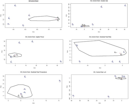
Batches are projected onto the IS CC showing five faulty batches outside the control region (Figure 13). In CO_j CCs, faulty batches are detected as out-of-control primarily in CCs corresponding to the perturbed variables. However, several batches whose variables didn’t suffer any modification, also signal out as faulty because of the correlation structure within the monitored variables (Figure 13).

Figure 13. IS and CO_j control charts for the fed-batch penicillin fermentation process. Points in black correspond to batches without shifts. The color used for batches exhibiting different levels of shifts is blue. The IS CCs showed five faulty batches, while the CO_j CCs evidenced several batches out of control according to perturbed variables and its correlation among other ones considered as part of the process.

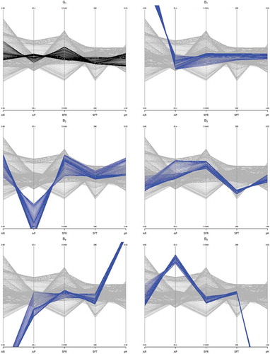
The described tendency can also be corroborated with parallel coordinate plotting, as shown in Figure 14, where just one good batch is plotted.

Figure 14. Parallel coordinate plots for the fed-batch penicillin fermentation process. Variables’ axes include AR = Aeration Rate, AP = Agitator Power, SFR = Substrate Feed Rate, SFT = Substrate Feed Temperature, and pH. Set of lines in black corresponds to batches without shifts. The color used for batches exhibiting different levels of changes is blue. Five batches evidenced an out-of-control condition.

4. Discussion

Our approach extends the work of Scepi (2002), where the use of the STATIS method in multivariate quality control was initially proposed. However, at least four contributions separate our proposal from the one presented in her work and others of similar importance. The first is related to preprocessing techniques applied to the raw data, the second is the DS-PC strategy to define the nonparametric control region, the third is the advantage of detecting different types of changes with the same CCs, and the fourth is the use of a well-known visual clustering method in multivariate process control as a diagnosis method for the out-of-control points signalized in the proposed CCs.

First, similar applications of STATIS extensions already published, consider for centering and later scaling the mean and standard deviation of each batch (Abdi et al., 2012; Filho & Luna, 2015) or simply do not include any criteria for this purpose, focusing on the normalization procedure (Niang et al., 2009). Instead, for our purpose, the data preprocessing is made considering the global mean and standard deviation of reference batches, complemented with normalization criteria. The normalization for all tables was performed dividing by number of rows of each table, which is the same in this example of Dual STATIS. This crucial step is extremely necessary to improve efficient detection of signals out of control (Abdi et al., 2012).

Second, the use of bagplot in quality control as a variant of the well-known convex hull peeling and B-spline smoothing is introduced in our proposal. Zani et al. (1998) applied convex hull peeling, which is somewhat less robust than half-space depth, as shown by Donoho and Gasko (1992). The notion of bagplots is based in Tukey’s half-space depth which has no restriction for any dimensions (Kruppa & Jung, 2017; Rousseeuw et al., 1999). The factor with which the bagplot is plotted poses another advantage of our proposal because the occurrence probability of false alarms is theoretically reduced to (Rousseeuw et al., 1999) leading in reduction of loss due to shrinkage.

Third, typically multivariate CCs’ detection of points out of control is due to several changes in the data, leading to complementary univariate analysis in order to reveal the type of shift responsible for the signal. In this sense, the use of several CCs is mandatory to address answers about shifts in mean, variability, and correlation structure (Bersimis et al., 2007; Montgomery, 2009). However, our work proposed here allows mean, standard deviation, and correlation shifts’ detection with one CC, IS CC for batches and CO_j CC for variables, where higher shifts produce greater detection.

Fourth, an original combination of an alternative analysis belonging to STATIS toolbox with Parallel Coordinates, is presented as a visual tool for detecting batches and variables out of control and identifying atypical behavior. The summarization of large multivariate data sets of both methods is enhanced due to control and monitoring application given here. Also, STATIS-based CCs plus parallel coordinate plots offer a representation, considering cross correlations of process variables besides means and standard deviations. Each shift can be interpreted as a result of different special or assignable causes depending on the process. Besides, such tools signalize out-of-control states precisely, leading to a smaller number of false alarms. As for our knowledge, similar studies haven’t considered this useful combination. Literature is full of techniques applied individually (Comfort et al., 2011; Dunia et al., 2012; Filho & Luna, 2015; Fogliatto & Niang, 2009; Niang et al., 2013, 2009).

Lately, research published in multivariate process control refers to time-wise analysis considering time instants within the batches (Filho & Luna, 2015; Fogliatto & Niang, 2009; Niang et al., 2013, 2009). These authors have already stated the variable-wise analysis as future research. However, none of them have already implemented the combined approach stated here. Other advantages of the proposed method are that the control and monitoring scheme for batch processes is nonparametric unlike other procedures, which widens its applicability to any case, without stablishing the data distribution. Usually, real data doesn’t follow an easy-to-use distribution making it difficult to control and monitor any process (Bersimis et al., 2007; Lewis, 2014).

Natural extensions of the work presented here include (i) a comparative study of IS and CO_j CCs obtained using the proposed method and others available in literature in terms of sensibility and statistical power; (ii) refinement of the method when shifts are introduced in several variables but not all of them; and (iii) development of the proposed charts to handle batches with missing values, which are common in practice. Research on real-time (on-line) variable-wise monitoring of batches, which was not addressed in our methodology, is currently in progress.

5. Conclusion

This paper presents a new approach to control multivariate processes in batch production, mixing Dual STATIS and Parallel Coordinates, without considering special constraints of data distribution. In addition, the construction of IS and CO_j CCs using robust bagplots for setting up control regions, allows to visualize changes in location, spread, and relationships between variables of data, signalizing greater fault detection as higher shifts take place. DS-PC strategy turns into a powerful tool for improving corrective actions and making important decisions in risk management.

On the other hand, the visualization of reference and new batches in the same plot with different parallel axis provides for an efficient analysis resource when an unusual behavior is detected, to identify mean, standard deviation, and correlation shifts and to search for extreme values that can occur in process’ variables during the production.

Although the control of a batch production process requires an elaborated statistical framework during the pilot and monitoring phase, there is no doubt that the original combination of visual resources proposed here, facilitate the inspection and identification of possible faulty batches and out-of-control variables, as previous step to the batches’ release.

Disclosure statement

No potential conflict of interest was reported by the authors.

References

- Abdi, H., Williams, L. J., Valentin, D., & Bennani-Dosse, M. (2012). STATIS and DISTATIS: Optimum multitable principal component analysis and three way metric multidimensional scaling. Wiley Interdisciplinary Reviews: Computational Statistics, 4(2), 124–167.
- Albazzaz, H. (2004). Statistical process control charts for batch operations based on independent component analysis. Industrial & Engineering Chemistry Research, 43(21), 6731–6741.
- Bersimis, S., Psarakis, S., & Panaretos, J. (2007). Multivariate statistical process control charts: An overview. Quality and Reliability Engineering International, 23(5), 517–543.
- Birol, G., Ündey, C., & Çinar, A. (2002). A modular simulation package for fedbatch fermentation: Penicillin production. Computers & Chemical Engineering, 26(11), 1553–1565.
- Comfort, J. R., Warner, T. R., Vargo, E. P., & Bass, E. J. (2011). Parallel coordinates plotting as a method in process control hazard identification. Proceedings of the 2011 IEEE Systems and Information Engineering Design Symposium (pp. 152–157). Charlottesville, VA, USA: University of Virginia.
- Doan, X.-T., & Srinivasan, R. (2008). Online monitoring of multi-phase batch processes using phase-based multivariate statistical process control. Computers & Chemical Engineering, 32(1–2), 230–243.
- Donoho, D. L., & Gasko, M. (1992). Breakdown properties of location estimates based on halfspace depth and projected outlyingness. The Annals of Statistics, 20(4), 1803–1827.
- Dunia, R., Edgar, T., & Nixon, M. (2012). Process monitoring using principal components in parallel coordinates. American Institute of Chemical Engineers Journal, 59(2), 1–12.
- Escoufier, Y. (1987). Three-mode data analysis: The STATIS method. In B. Fichet & C. Lauro (Eds.), Methods for multidimensional data analysis (pp. 259–272). Napoli: ECAS.
- Filho, D., & Luna, L. (2015). Multivariate quality control of batch processes using STATIS. The International Journal of Advanced Manufacturing Technology, 82(5), 867–875.
- Flores-Cerrillo, J., & MacGregor, J. F. (2002). Control of particle size distributions in emulsion semibatch polymerization using mid-course correction policies. Industrial and Engineering Chemistry Research, 41(7), 1805–1814.
- Fogliatto, F. S., & Niang, N. (2009). Multivariate statistical control of batch processes with variable duration. IEEE International Conference on Industrial Engineering and Engineering Management (pp. 434–438). Hong Kong, China: IEEE.
- Gabriel, K. R. (1971). The biplot graphic display of matrices with application to principal component analysis. Biometrika, 58(3), 453–467.
- Galindo, P. (1986). Una alternativa de representación simultánea: HJ-Biplot. Qüestiió: Quaderns d’Estadística, Sistemes, Informatica I Investigació Operativa, 10(1), 13–23.
- Golub, G., & Van Loan, C. (1996). Matrix computations (3rd ed.). Baltimore & London: Johns Hopkins University Press.
- Gower, J., Gardner-Lubbe, S., & le Roux, N. (2011). Understanding biplots. UK: John Wiley & Sons.
- Hanyuan, Z., & Xuemin, T. (2017). Batch process monitoring based on batch dynamic Kernel slow feature analysis. Proceedings of the 29th Chinese Control and Decision Conference, CCDC 2017, 5 (pp. 4772–4777). Chongqing, China: IEEE.
- Harris, T. C., Seppala, C. T., & Desborough, L. D. (1999). A review of performance monitoring and assessment techniques for univariate and multivariate control systems. Journal of Process Control, 9(1), 1–17.
- Heinrich, J., & Weiskopf, D. (2013). State of the art of parallel coordinates. In Eurographics Conference on Visualization (Eurovis) (pp. 95–116). Leipzig, Germany: IEEE.
- Horn, R., & Johnson, C. (2013). Matrix analysis (2nd ed.). New York, NY, USA: Cambridge University Press.
- Hotelling, H. (1947). Multivariate quality control illustrated by air testing of sample bombsights. In C. Eisenhart, M. W. Hastay, & W. A. Wallis (Eds.), Techniques of statistical analysis (pp. 111–184). New York, NY: McGraw Hill.
- Inselberg, A. (2009). Parallel coordinates: Intelligent multidimensional visualization (D. Plemenos & G. Miaoulis, Eds.). Berlin, Heidelberg: Springer.
- Inselberg, A., & Dimsdale, B. (1990). Parallel coordinates: A tool for visualizing multi-dimensional geometry. Proceedings of the First IEEE Conference on Visualization (pp. 361–378). San Francisco, CA, USA: IEEE.
- Jackson, J. E. (1991). A User’s Guide to Principal Components. (Vol. 26). USA: John Wiley & Sons.
- Jackson, J. E., & Mudholkar, G. S. (1979). Control procedures for residuals associated with principal component analysis. Technometrics, 21(3), 341–349.
- Kourti, T. (2003). Multivariate dynamic data modeling for analysis and statistical process control of batch processes, start-ups and grade transitions. Journal of Chemometrics, 17(1), 93–109.
- Kourti, T., & MacGregor, J. F. (1996). Multivariate SPC methods for process and product monitoring. Journal of Quality Technology, 28(4), 409–428.
- Kourti, T., Nomikos, P., & MacGregor, J. F. (1995). Analysis, monitoring and fault diagnosis of batch processes using multiblock and multiway PLS. Journal of Process Control, 5(4), 277–284.
- Kruppa, J., & Jung, K. (2017). Automated multigroup outlier identification in molecular high-throughput data using bagplots and gemplots. BMC Bioinformatics, 18(232), 1–10.
- L'Hermier des Plantes, H. (1976). Structuration des Tableaux à Trois Indices de la Statistique: Théorie et Application d’une Méthode d’ Analyse Conjointe. Université des Sciences et Techniques du Languedoc, Montpellier.
- Lange, B., Rodriguez, N., Puech, W., & Vasques, X. (2011). Visualization assisted by parallel processing. Parallel Processing for Imaging Applications. San Francisco, CA, USA: SPIE.
- Lavit, C., Escoufier, Y., Sabatier, R., & Traissac, P. (1994). The ACT (STATIS method). Computational Statistics & Data Analysis, 18(1), 97–119.
- Lee, J. M., Yoo, C. K., & Lee, I. B. (2004). Fault detection of batch processes using multiway kernel principal component analysis. Computers and Chemical Engineering, 28(9), 1837–1847.
- Lewis, D. (2014). Control charts for batch processes. Wiley StatsRef: Statistics Reference Online, 1–9. Lake Oswego, OR, USA: John Wiley & Sons.
- Liu, R. Y. (1995). Control charts for multivariate processes. Journal of the American Statistical Association, 90(432), 1380–1387.
- Liu, R. Y., & Tang, J. (1996). Control charts for dependent and independent measurements based on bootstrap methods. Journal of the American Statistical Association, 91(436), 1694–1700.
- Lombardo, R., Vanacore, A., & Durand, J. (2008). Non parametric control chart by multivariate additive partial least squares via spline. In C. Preisach, H. Burkhardt, L. Schmidt-Thieme, & R. Decker (Eds.), Data analysis, machine learning and applications: Proceedings of the 31st annual conference of the Gesellschaft für Klassifikation (pp. 201–208). Berlin Heidelberg: Springer-Verlag.
- Lowry, C. A., & Montgomery, D. C. (1995). A review of multivariate control charts. IIE Transactions, 27(6), 800–810.
- Macgregor, J. F. (1997). Using on-line process data to improve quality: Challenges for statisticians. International Statistical Review, 65(3), 309–323.
- Montgomery, D. (2009). Introduction to statistical quality control. Hoboken, NJ, USA: John Wiley & Sons.
- Næs, T., Brockhoff, P. B., & Tomic, O. (2010). Statistics for sensory and consumer science. London: John Wiley & Sons.
- Narayanachar, P. (2013). R statistical application development by example beginner’s guide. UK: Packt Publishing Ltd.
- Niang, N., Fogliatto, F., & Saporta, G. (2009). Batch process monitoring by three-way data analysis approach. The XIIIth International Conference on Applied Stochastic Models and Data Analysis (pp. 463–468). Vilnius, Lithuania: ASMDA International.
- Niang, N., Fogliatto, F. S., & Saporta, G. (2013). Non parametric on-line control of batch processes based on STATIS and clustering. Journal de La Société Francaise de Statistique, 154(3), 124–142.
- Nomikos, P., & MacGregor, J. F. (1995). Multivariate PSC charts for monitoring batch processes. Technometrics, 37, 41–59.
- Rousseeuw, P. J., Ruts, I., & Tukey, J. W. (1999). The bagplot: A bivariate boxplot. American Statistician, 53(4), 382–387.
- Scepi, G. (2002). Parametric and non parametric multivariate quality control charts. In C. Lauro, J. Antoch, V. E. Vinzi, & G. Saporta (Eds.), Multivariate total quality control: Foundation and recent advances (pp. 163–189). Heidelberg: Physica-Verlag HD.
- Trefethen, L., & Bau, D. (1997). Numerical linear algebra (1st ed.). Philadelphia: Society for Industrial and Applied Mathematics.
- Tucker, L. R. (1964). The extension of factor analysis to three-dimensional matrices. In H. Gulliksen & N. Frederiksen (Eds.), Contributions to mathematical psychology (pp. 110–182). New York, NY: Holt, Rinehart & Winston.
- Wang, X., Medasani, S., Marhoon, F., & Albazzaz, H. (2004). Multidimensional visualization of principal component scores for process historical data analysis. Industrial & Engineering Chemistry Research, 43(22), 7036–7048.
- Wegman, E. (1990). Hyperdimensional data analysis using parallel coordinates. Journal of the American Statistical Association, 85(411), 664–675.
- Westerhuis, J. A., Kourti, T., & MacGregor, J. F. (1998). Analysis of multiblock and hierarchical PCA and PLS models. Journal of Chemometrics, 12, 301–321.
- Wierda, S. J. (1994). Multivariate Statistical Process Control - recent results and directions for future research. Statistica Neerlandica, 48(2), 147–168.
- Yoo, C. K., Lee, J. M., Vanrolleghem, P. A., & Lee, I. B. (2004). On-line monitoring of batch processes using multiway independent component analysis. Chemometrics and Intelligent Laboratory Systems, 71(2), 151–163.
- Zani, S., Riani, M., & Corbellini, A. (1998). Robust bivariate boxplots and multiple outlier detection. Computational Statistics and Data Analysis, 28(3), 257–270.