Inventory strategy for spare parts redundancy to support server operations during production processes

ABSTRACT

Inventory strategies are very necessary for supporting the production process. The strategy in the form of a model is proposed for redundant allocation of critical parts of a server system for minimizing additional costs. This model considers the occurrence of failure using downtime limits as the downtime on the server should be minimal. The rapid replacement of spare parts can be achieved through an onsite inventory or a redundant configuration. Furthermore, fast delivery would be an alternative when there is no inventory or redundancy. We considered four scenarios including a combination of stock, installation of redundant components, and fast deliveries. The model was solved using the Lagrangian relaxation method. No downtime in scenarios using redundancy resulted in a stable total cost over the last period, even though the penalty increased. The redundant module only had an additional cost in the initial period, so if the penalty value increased, there was a switching of scenario selection in the third or fourth scenario.

KEYWORDS:

• Inventory
• critical spare parts
• downtime
• redundant component

1. Introduction

The management of spare parts is complex. Spare part management is required to ensure high reliability, availability of parts and equipment operation. Avoiding and anticipating equipment damage is possible through maintenance and installation of redundant parts. The risk of failure can potentially be reduced through planned maintenance and redundancy, thus prolonging the life of the system and reducing costs associated with repairs. If failure is inevitable, it is important to reduce downtime by ensuring that the needed spare part is available. Giri and Dohi (2009) analysed the inventory control policy considering an emergency order for providing a balance between economy and reliability. They applied cost-effectiveness criteria, including the effects of system availability and expected costs to obtain an optimal inventory. Kennedy, Patterson, and Fredendall (2002) reviewed research papers on inventory of spare parts. Boylan and Syntetos (2010) undertook a review on spare parts management based on strategies for sharing demand information and the design of forecast support systems. Hu, Boylan, Chen, and Labib (2018) conducted spare part management reviews based on the product life cycle process, objectives, and main tasks to support spare parts inventory in Operations Research fields.

Studies on inventory theory have indicated the importance of effective management of spare parts. Spare parts management is a design-oriented process, with planning and control of information and the flow of parts (Hellingrath & Cordes, 2014). The forecasting method was developed for increasing the estimate of demand for parts to enhance the methods for supply chain planning and collecting condition monitoring information. While the availability of parts is critical, inventory is also costly to hold, and hence it is very important to achieve minimum costs and downtime. The problem becomes more complex owing to uncertain demands. Demand for spare parts occurs because of failure and procurement lead time is lengthy. In addition, spare part inventory is always characterized by uncertain demand. Basten & van Houtum (2013) integrated a single-location model with emergency shipment as well as a two-echelon model with an emergency shipment. Service-oriented systems are generally used in spare parts inventory control because downtime is expensive. The effect of location is called spatial dependence in deciding the allocation of spare parts inventories in multi-echelon systems (Lukitosari, Suparno, Pujawan, & Widodo, 2016). Driessen, Arts, van Houtum, Rustenburg, and Huisman (2010) stated that a business relying heavily on the availability of equipment should avoid downtime because it can cause harm in the form of (i) loss in sales; (ii) customer dissatisfaction allowing a claim; and (iii) safety risk.

Therefore, we contribute toward improving inventory strategies by proposing a new inventory model for ordering spare parts, showing the usability of redundancy. When system availability is critical, there are three choices for companies. The first one is to provide a redundant unit where, when the primary part fails, the redundant unit will take over. The use of redundant parts extends into any complex systems such as those used in aircraft, telecommunications, computation, submarines, military weapons, and nuclear systems. The second one is to have the part as an inventory. This would be different from the redundant unit as it is not directly installed in the system, but it is available onsite as inventory stored in the warehouse. Having spare parts installed as a redundant system or as inventory in the warehouse would imply inventory costs as the company has to purchase the spare part in advance, thus incurring capital costs. The third option is to have a fast replenishment or supply system from the spare part centre or a supplier. Here, the replenishment of the spare part starts when the system fails. This option is preferable when the spare part is expensive, but only feasible when the supply lead time for a new spare part is very short.

The use of the above alternatives separately has been discussed in earlier studies. The use of inventory has attracted much attention in studies regarding spare parts inventory. Researchers have also examined the use of standby spare parts, but the number is quite limited as this may not be always applicable in any system. Several studies have addressed issues related to redundant parts (Cochran & Lewis, 2002; van Jaarsvel & Dekker, 2011; Chambari, Habib, Rahmati, & Abbas, 2012; Safari, 2012). Cochran and Lewis (2002) conducted case studies on the application of military aircraft in the Gulf War. For obtaining a quick response, it is required that spare parts are always available. There are some spare parts in aircraft engines installed as redundant parts, and others are always ready in warehouse as onsite stock.

There are researchers studying the configuration of redundant equipment where the equipment operates with at least k components out of n existing components in the system. For example, Dohi, Osaki, and Kaio (1996) examined the optimal spare part ordering policies for a cold standby redundant system with two dissimilar units. Coit and Liu (2000) examined approaches to improve the reliability and availability of systems through redundancy. This was later extended by Ramirez-Marquez, Coit, and Konak (2004), who proposed a methodology to optimize the allocation of components through the logic of increasing the reliability of the system by minimizing failure time. de Smidt-Destombes, van Der Heijden, and van Harten (2009) analysed redundant parts inventory and capacity improvement in a condition-based maintenance scenario. Spare parts consisted of identical components in the system k-out-of-n and could be repaired if damaged. The study used a heuristic method to obtain a cost-effective scenario to reach a balance between the frequency of maintenance, spare parts inventory and repair capacity. Eryılmaz (2009) improved the reliability of redundant parts with arbitrary lifetime distributions. de Smidt-Destombes, van Elst, Isabel, Mulder, and Hontelez (2011) also emphasized the cost-effective spare parts in stock and increased costs due to redundancy. Aghaei, Hamadani, and Ardakan (2016) developed a strategy for solving the redundancy problem through a modified version of the genetic algorithm, resulting in improved reliability levels.

The present study was motivated by the challenges faced when using information systems in the production process. Reliable servers should support information systems that have stringent standards regarding downtime tolerance. Servers comprise a large number of components that may fail at some point in time. Therefore, management in term of the provision of spare parts is required. Spare parts inventory guarantees a fluent production process. On the other hand, excessive inventory is an expensive solution, especially for critical components. Specific challenges involved in the logistics of spare parts, in addition to high penalties for downtime, attract attention in integrating stock availability, redundancy and fast delivery to address spare part management issues. To the best of our knowledge, the trade-off between inventory and downtime related to redundancy and delivery has never been discussed. This paper introduces a model and scenarios in terms of availability and cost. The three key aspects considered in this study were stock availability, redundancy, and fast delivery.

Some studies that discuss spare parts strategy involving redundancy, availability, and downtime functions. However, no one has considered the situation that we discussed in this study. Table 1 presents a summary of the existing studies and the relevance of this study.

Table 1. Studies on redundancy of spare parts.

Author(s)	Failure of critical component	Availability spare part	Decision variables	Objective	Comparison
Coit & Liu (2000)	Exponential distribution	No onsite stock, Active or cold standby	Components used for subsystems	Max Reliability	Solution of Fyffe et al.(1968)
Ramirez-Marquez et al. (2004)	Failure independent, no distribution	Resources globally available to fairly allocate subsystem reliability	Components used for subsystems.	Max–min Reliability	Genetic Algorithm
Eryılmaz (2009)	Multivariate lifetime distribution	No onsite stock	Formulas for survival, MTTF, failure rate, and mean residual lifetime.	Formulas for reliability characteristics	Numerical exampled for variation of k- out- of-n
de Smidt-Destombes et al. (2011)	Exponential distribution	Minimal spares, same as cold standby	Demand for item and probability of availability during the operating time	Cost- effective spare parts package	Approximation method and exact method
Jaarsveld & Dekker, 2011	Exponential distribution, Erlang distribution	Onsite stock, cold standby & hot standby	Stock decision Reorder points	Min downtime cost & shortage costs	Traditional inventory methods: data regarding redundancy is not available
Chambari et al., 2012	Erlang distribution, exponential	Unlimited stock, active or cold standby	System-level configuration Selection of component type, active- and cold-standby strategies.	A bi-objective model: Max reliability & Min cost.	Non-dominated sorting genetic algorithms (NSGA-II) and multi-objective particle swarm optimization (MORAP)
Safari, 2012	Erlang distribution	No onsite stock, active or cold standby	The number and component choice used for a subsystem Active/cold standby	Multi-objective: Max reliability & Min cost	Genetic algorithm for the single-objective redundancy allocation problem (SORAP)
Kim & Kim (2017).	Exponential distribution	No onsite stock, active or cold standby	Component reliability Redundancy levels for individual subsystems	Max reliability using a parallel genetic algorithm	Genetic algorithm
Aghaei et al. (2016)	Exponential distribution	No onsite stock, active and cold standby	Number of components Type of component Active and cold standby	Max reliability	Solution of Fyffe et al.(1968) & Coit & Liu (2000)
Proposed Model	FMEA Exponential distribution, Erlang distribution	Combination of onsite stock, cold standby & fast delivery	Redundancy Stock decision Amount of stock	Min cost	Analytical hierarchy process

2. System description

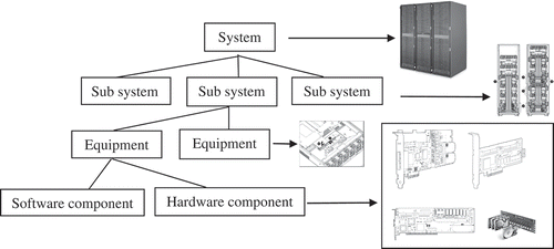
This was a quantitative study conducted on companies, whose production data are managed with good information technology, making this research very valuable for comparing costs and downtime in the model. The focus was on an important server in the production process. The production process could be more systematic and monitored by the server. Every production process including purchase orders, assemblies, project orders, material releases, and delivery orders can be monitored quickly and comprehensively. A server system is a group of modules combined into one to achieve the desired goal, i.e., minimal costs and limited downtime. The modules consist of several components, depicted in Figure 1. A component consists of hardware and software. The hardware in this context comprises the spare parts for supporting the server. The availability of spare parts supports production continuity. One important finding of this study was that a system must recover very quickly when one of the spare parts fails. This can be achieved in three ways: (i) redundancy so that the redundant part can directly take over when the other one fails; (ii) having onsite stock to support replacement of the failed spare part; or (iii) fast delivery from the supplier to ensure the server does not experience downtime beyond the tolerance limit.

Figure 1. Server system with its components.

We considered inventory based on redundancy or onsite stock for a spare part server. Redundancy refers to identical spare parts or two units of the same components that are connected in parallel, while onsite stock refers to the unit near a server. We considered the speed of repairing the system using the concept of repair-by-replacement. That is, if a spare part fails and causes system failure, the system will be restored using the redundant part (if there is a redundant part installed) or replaced by a new part available in the inventory.

Server spare parts inventory management was applied to complex systems to support data processing in manufacturing companies producing bicycles. A server as a data service centre for a large company is generally used as a storage medium for all data from a client server that can be accessed at any time automatically. The purpose of a server is to simplify and speed up work on a system in a particular job. In a network server system equipped with a database server, all data or documents stored on the server can be accessed by other parts when required.

In the bicycle industry, manufacturing digitization through digital transformation involves changing operating manuals, handbooks, documents and other sources of information into a digital format. The process is a major breakthrough in terms of efficiency, allowing the server to search, access, store, exchange and integrate all the data. The use of digital information to optimize production workflows makes it simpler, more efficient and cost-effective.

Supply chains can be integrated with servers to reduce inventory and increase just-in-time manufacturing inventory. Production control involves welding-painting-assembly-inspection-packaging processes; for example, waste in welding often occurs because of over processing, reworking and defective frames and forks. The server stores big data pertaining to the quality of production; then identification and design can be performed to minimize waste generation in the bicycle production process.

We considered failure mode and effect mode (FMEA) as a tool to determine critical components that must be stocked or carried out redundancy. FMEA is used as a risk assessment tool to determine the threshold for the level of risk that is acceptable. FMEA can identify potential failure points are in an information technology environment (Gan, Xu, & Han, 2012). Potential failures are identified before they become a problem. Server failure impacts the production process; it affects records on incoming material data, damaged material, process data and outgoing material.

The server component is represented physically in a module. Modules are ranked in the FMEA process to identify critical components as a sequence of risks from major failures. The FMEA team calculates the value of severity (SEV), occurrence (OCC) and detection (DET) based on the scale proposed by Stamatis (2003). The FMEA method is used to determine the risk priority number (RPN). The RPN is obtained by multiplying SEV, OCC and DET. The highest RPN value occurring on the hard disk during failure caused by an electrical disturbance is 243. There are five largest RPN values, which are priorities for regular control actions in the server system presented in Table 2. The function of the server in a network system is very vital. The server can process data requests quickly from the client server that is connected to it. All server components must consist of components with high specifications, including the hard disk, processor, RAM, power supply and main board. The component is a module or subsystem of the server.

Table 2. Risk analysis and ranking of RPN.

No.	Module	Function	Failure Modes	Failure Cause	Effect	Controls	SEV	OCC	DET	RPN
1	Hard disk	Data storage	Data loss	Electrical disturbances, magnetic field around the server.	Data is not accessible.	Use of UPS and generator to deal with unstable electricity voltage. Objects that have magnetic fields are kept away from the server.	9	3	9	243
2	Power Supply	Voltage/current power supply to all hardware parts.	The server can be turned on but it will not work for long.	Excessive load and unstable voltage	Power supply failure	Load balancing, check indicator of the lamp (led), electric stabilizer and age of use of the power supply.	8	4	7	224
3	RAM	Temporary data storage	The server sounds abnormal.	Corrosion caused by dust and mildew in RAM socket.	The server hangs.	Check RAM	9	5	4	180
4	Main board	Main circuit board, connector of the server components	The monitor indicator blinks even though the fan of the power supply and processor work, but the OS does not work.	The chip and transistor components burn.	Mainboard failure	Check chip (IC), transistors and programs in firmware.	8	3	7	168
5	Processor	Brain and control.	The program and OS server do not work.	Fan speed decreases or fan is damaged.	The server hangs	Check slot and jumper of processor.	4	7	6	168

We propose four scenarios in Section 3.3. The scenarios include combinations of stock, redundancy and fast delivery. Each scenario gives a different downtime expectation. In addition, each scenario has different cost consequences. The proposed scenarios represent different alternatives for maintaining system reliability. Obviously, each of these combinations may be expected to perform well under different situations. For example, the use of redundant or onsite stock would be preferable when a spare part is expensive, and immediate supply from the supplier requires a longer time than the tolerance time limit. The four proposed scenarios are compared with the multicriteria analytical hierarchy process (AHP) in the result and discussion section. The AHP may be a powerful tool in the context of decision making, assisting in situations with several dependent (alternative decisions) and independent variables (decision criteria) (Hofmann & Knébel, 2013; Kabir & Sumi, 2014).

3. Model development

3.1. Previous model

Several publications are closely related to our work, including those related to optimization models (Bien, 1971; Coit & Liu, 2000; Kim & Kim, 2017). Generally, the redundant parts allocation problem aims to maximize system reliability $R\left(t\right)$. The objective is to select the components and redundancy levels to maximize system reliability, given certain system-level constraints. There are two constraints, namely a specified budget and the amount of data that can be accommodated. Another model is based on the works of de Smidt-Destombes et al. (2009) and Kim and Kim (2017) with the aim of minimizing the expected cost per unit of time. Several studies on optimization use formulations with common forms as expressed in Equation (1) (Kuo & Wan, 2007; Ravindran, Ragsdell, & Reklaitis, 2006).

(1) $\begin{array}{rl}& \mathrm{M}\mathrm{a}\mathrm{x}\mathrm{i}\mathrm{m}\mathrm{i}\mathrm{z}\mathrm{e}\mathrm{o}\mathrm{r}\mathrm{M}\mathrm{i}\mathrm{n}\mathrm{i}\mathrm{m}\mathrm{i}\mathrm{z}\mathrm{e}:f\left(\mathit{x}\right)\\ & \mathrm{s}\mathrm{u}\mathrm{b}\mathrm{j}\mathrm{e}\mathrm{c}\mathrm{t}\mathrm{t}\mathrm{o}g\left(\mathit{x}\right)\le b_i\mathrm{f}\mathrm{o}\mathrm{r}i\in \left\{1,2,3,\dots ,z\right\},\\ & \mathit{x}\in \mathit{X}\end{array}$(1)

Equation (1) provides the objective function $f\left(\mathit{x}\right)\mathrm{f}\mathrm{o}\mathrm{r}$ the reliability–redundancy allocation problem by maximizing reliability or minimizing costs; $g\left(\mathit{x}\right)$ represents the constraints, and $\mathit{x}$ represents decision variables.

3.2. Proposed model

The framework of the optimization model was developed by referring to the model proposed in Section 3.1; however, this study differed slightly in the scenario regarding the availability of spare parts and downtime constraints. The reliability of the server was maintained with the availability of spare parts useful for critical engine parts having uptime within a certain tolerance level.

3.2.1. Problem formulation

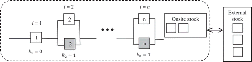
In this study, we used redundancy to improve reliability by replicating a single unit with two units of the same components or spare parts. We consider a system composed of multiple subsystems i (henceforth called module i). Each module consists of a unit (without redundancy, it has only one unit) or two similar units. A module consists of two units; while the first unit starts operating, the second unit acts as a redundant unit. When the primary unit fails, the redundant unit starts to operate with perfect switching. A redundant part is a cold spare part. In a design with module i, the two-unit redundant parts are connected in parallel to one another, and each module is connected in series, as illustrated in Figure 2 (second unit shaded to indicate redundant unit). Spare part stock can also be ensured by providing units onsite. The module consists of one spare part when $k_i=0$, which implies that the module is without redundancy.

Figure 2. Model description.

We employed the following assumptions: The system operates 24 hours a day without stopping. Repairs are performed by replacing the defective parts with new ones; there is no dependency between the failures of components. The failure of spare parts follows a Poisson process while the lifetime of spare parts follows an exponential distribution. The repair time includes both the repair time itself and delivery time.

The following are the decision variables:

$x_{1i}$ : number of onsite stock units for module i

$x_{2i}$ : 0–1, variable that is equal to 1 if redundancy for module i is established and 0 otherwise

$x_{3i}$ : 0–1, variable that is equal to 1 if onsite stock is available for module i and 0 otherwise

Notations

i : set of modules with index i

$k_i$ : redundant part for module i

$T$ : expected lifetime of system based on exploitation time of server

α : annual discount rate

${\lambda }_i$ : failure arrival rate of module i

$P_{x_{1i}}$ : out of stock probability for module i

$a_i$ : purchasing cost per unit of module i

$b_i$ : cost due to redundancy of module i

$c_i$ : costs of replacement for module i

$d_i$ : cost of transportation for module i from external stock via fast delivery

$h_i$ : holding cost rate per unit i

$t_{1i}$ : mean replacement time of damaged module i with onsite stock

$t_{2i}$ : mean replacement time of damaged module i via fast delivery from external stock

$D$ : downtime (hours)

T_m : maximum tolerable downtime

3.2.2. Repair and cost of spare parts

Repair was performed by replacing damaged parts with new ones. We assumed that the totally damaged parts follow a Poisson distribution, with arrival rate λ_i, and service rate µ_i. The process involving spare parts inventory is considered identical to a queuing process (Baskett, Chandy, Muntz, & Palacios, 1975). The arrival of spare parts represents the demand due to failure. The behaviour of the physical stock is identical with the out of stock probability according to the Erlang formula (Kranenburg & van Houtum, 2007; van Jaarsvel & Dekker, 2011). This is the celebrated Erlang’s loss formula, derived by A.K. Erlang in 1971, denoted as follows:

(2) $P_{x_{1i}}={\left(\frac{{\lambda }_i}{{\mu }_i}\right)}^{x_{1i}}\frac{P_0}{x_{1i}!}=\frac{{\left(\frac{{\lambda }_i}{{\mu }_i}\right)}^{x_{1i}}\frac{1}{x_{1i}!}}{{\sum }_{j=0}^{x_{1i}}{\left(\frac{{\lambda }_i}{{\mu }_i}\right)}^j\frac{1}{j!}}$(2)

Suppose that the demand of parts follows a Poisson process. Failures occurring in each of the parts are independent. The lifetime of the product follows an exponential distribution (Cochran & Lewis, 2002; Coit & Liu, 2000; Graves, 1985). Analysis of the failure of parts is assumed to be performed accurately, and the analysis time is negligible. If the module failure can be considered as a Poisson process with rate λ_i throughout [0, T], then the mean time between the failures of module i is θ_i. We applied the mean replacement time of the damaged module with external stock via fast delivery such that it was higher than the mean replacement time of the damaged module with onsite stock.

The model was built considering optimization issues and aimed at minimizing total additional costs. Four types of costs were included in this study. First, the purchase cost of spare parts i during [0, T] was considered, with $a_i$ being the cost per unit spare part; this can be expressed as

(3) $f_1=\sum _{i=1}^n{a}_i{x}_{1i}$(3)

Second, the cost emerging from redundancies results in additional cost $b_i$ for parts i in the system. Additional charges do not appear when the module is not installed redundantly:

(4) $f_2=\sum _{i=1}^n{b}_i{x}_{2i}.$(4)

Third, the holding cost of spare parts i is considered, where the holding cost is the average cost per part i, and the cost of holding one part throughout its lifetime is [0, T] using a discount $\propto >0$:

(5) $f_3=\sum _{i=1}^n\frac{h_i}{\propto }{x}_{1i}\left(1-ex{p}^{-\propto T}\right)$(5)

Fourth, the cost of replacement for parts i during [0, T] was considered. In the event of failure, if the stock is available, then the damaged part is replaced with onsite stock. If the stock is not available, then the fast delivery mode will be activated, and the new part from external stock replaces the failed part. $c_i$ includes all costs of the replacement procedure applied for module i, which are repair costs and administrative costs of failed part i. Moreover, $d_i$ is defined as the fast transportation cost from external stock. We assumed $d_i$ to be much larger than $c_i$. The replacement cost was formulated as follows:

(6) $f_4=\sum _{i=1}^n\frac{1}{\alpha {\theta }_i}\left(1-ex{p}^{-\alpha T}\right)\left\{c_i+d_i\left(1-x_{3i}\right)P_{x_{1i}}\right\}.$(6)

We developed the critical spare parts inventory model that considers redundancy with the goal of minimizing additional costs. We formulated the problem using Equations (3), (4), (5) and (6) as follows:

(7) $\mathrm{M}\mathrm{i}\mathrm{n}\mathrm{i}\mathrm{m}\mathrm{i}\mathrm{z}\mathrm{e}C=f_1+f_2+f_3+f_4$(7)

3.3. Spare parts ordering scenario and expectation of downtime

We developed inventory and redundancy scenarios where each scenario was reviewed for downtime. The model was built with four scenarios that are a combination of stock and redundancy as follows:

1. In the first scenario, inventories of spare parts were used to replace the damaged parts; therefore, it was not necessary to order the part via fast delivery. In this scenario, the server was not installed using redundant parts. There was failure due to damage to the parts. The length of the expected downtime depended on the mean replacement time of the damaged parts, $t_{1i}$, amounting to $D_1=t_{1i}\frac{T}{{\theta }_i}$.

2. The second scenario did not involve stock or redundant parts, so fast delivery was used to replace damaged parts. When inevitable failure occurred, downtime due to waiting parts occurred and repair started as soon as the part arrived. The time needed for making fast or urgent deliveries was $t_{2i}\frac{T}{{\theta }_i}{P_x}_{1i}$. The duration of downtime for replacement of damaged parts was calculated as $t_{1i}\frac{T}{{\theta }_i}$, so the total of the downtime occurring during [0, T] in the second scenario was calculated as $D_2=t_{2i}\frac{T}{{\theta }_i}{P_x}_{1i}+t_{1i}\frac{T}{{\theta }_i}$.

3. In the third scenario, there was a redundant part but no onsite stock. When damage occurred, the system was still operational. A newly ordered part was assumed to be procured via fast delivery. In this scenario, the server did not experience downtime, so $D_3=0$.

4. The fourth scenario was similar to the third one, but fast deliveries were not applicable here. Spare parts were installed in the redundant module if there was damage to one of the parts; the system could still operate because there was a redundant part. However, because the server part was critical, there was also onsite stock. In this scenario, there was no downtime, so $D_4=0$.

Based on the four scenarios involving ordering spare parts and downtime obtained above, the expected downtime constraint is given by the following equation:

(8) $D=\sum _{i=1}^n\frac{T}{{\theta }_i}\left(1-x_{2i}\right)\left[t_{1,i}+t_{2,i}\left(1-x_{3i}\right){P_x}_{1i}\right].$(8)

Expected failure of the model that occurred throughout $\left[0,T\right]$ did not exceed the maximum of the tolerable downtime T_m. Then,

(9) $D\le T_m.$(9)

3.4. Solving the problem

The spare parts ordering scenario, described in Section 3.3, was included in the model formulation. In the first step, the ordering scenarios are defined by 0–1 decision variables $x_{2i},x_{3i}$ as follows:

(10) $x_{2i}=\left\{\begin{array}{c}1,ifbuildingredundancyformodulei\\ 0,otherwise\end{array}\right.$(10)

$x_{3i}=\left\{\begin{array}{c}1,ifonsitestockformodulei\\ 0,otherwise\end{array}\right.$

Spare part stock is controlled by a continuous review policy. The total inventory includes the onsite stock and pipeline stock parts i specified by

(11) $x_{1i};x_{1i}\in \left\{0,1,2,\dots \right\}.$(11)

In the second step, the technique used to solve the objective function of Equation (7) and constraints (9)–(11) is the Lagrangian relaxation method (Everett, 1963). The Lagrange and Kuhn–Tucker theory provides a powerful motivation and theoretical basis for the methods considered here.

$\mathrm{M}\mathrm{i}\mathrm{n}\mathrm{i}\mathrm{m}\mathrm{i}\mathrm{z}\mathrm{e}:L\left(x;v\right)=\sum _{i=1}^n{a}_i{x}_{1i}+\sum _{i=1}^n{b}_i{x}_{2i}+\sum _{i=1}^n\frac{h_i}{\propto }{x}_{1i}\left(1-ex{p}^{-\propto T}\right)+\sum _{i=1}^n\frac{1}{\alpha {\theta }_i}\left(1-ex{p}^{-\alpha T}\right)\left\{c_i+d_i\left(1-x_{3i}\right)P_{x_{1i}}\right\}+v\left[\sum _{i=1}^n\frac{T}{{\theta }_i}\left(1-x_{2i}\right)\left[t_{1,i}+t_{2,i}\left(1-x_{3i}\right){P_x}_{1i}-T_m\right]\right].$

Here, $v$ is the Lagrange multiplier.

$L\left(x;v\right)$ is a supply function for many modules; therefore, this function can be simplified into a one-module inventory function with the following decomposition:

$L\left(x;v\right)=a_i{x}_{1i}+b_i{x}_{2i}+\frac{h_i}{\propto }{x}_{1i}\left(1-ex{p}^{-\propto T}\right)+\frac{1}{\alpha {\theta }_i}\left(1-ex{p}^{-\alpha T}\right)\left\{c_i+d_i\left(1-x_{3i}\right)P_{x_{1i}}\right\}+v\left[\frac{T}{{\theta }_i}\left(1-x_{2i}\right)\left[t_{1,i}+t_{2,i}\left(1-x_{3i}\right){P_x}_{1i}-T_m\right]\right]$

.

The optimal solution is obtained in accordance with the change in the objective function, directly proportional to the downtime constraint change, with the Lagrange $\mathrm{m}\mathrm{u}\mathrm{l}\mathrm{t}\mathrm{i}\mathrm{p}\mathrm{l}\mathrm{i}\mathrm{e}\mathrm{r}v.$ In the implementation, Lagrange multipliers can be described as penalty functions. The constrained optimization problem is converted to a problem without limitations through the penalty function $v.$ The structure of the penalty function for updating the penalty parameters at the end of each unconstrained minimization stage defines the particular method. The penalty function is exact if only one unconstrained minimization is required (Ravindran et al., 2006).

Derivatives of the functions of real variables measure the sensitivity to changes in the values of cost functions with respect to changing input values. The derivative of the cost changes to that of the downtime, with respect to the choice of scenario; it measures how quickly the cost position changes when the downtime alters. The first derivatives are as follows:

(12) $\frac{\mathrm{\partial }L}{\mathrm{\partial }{x}_{2i}}=b_i-v\left[\frac{T}{{\theta }_i}\left[t_{1,i}+t_{2,i}\left(1-x_{3i}\right)P_{x_{1i}}-T_m\right]\right]=0.$(12)

(13) $\frac{\mathrm{\partial }L}{\mathrm{\partial }v}=\left[\frac{T}{{\theta }_i}\left(1-x_{2i}\right)\left[t_{1,i}+t_{2,i}\left(1-x_{3i}\right){P_x}_{1i}-T_m\right]\right]=0$(13)

From Equations (12) and (13), we determined the penalty function as follows:

(14) $v=\frac{b_i}{\frac{T}{{\theta }_i}\left[t_{1,i}+t_{2,i}\left(1-x_{3i}\right)P_{x_{1i}}-T_m\right]}.$(14)

We found the value of the maximum tolerable downtime ($T_m)$ to be part of the penalty.

4. Numerical example

An illustrative example is provided to explain the following case: The server requires the availability of spare parts, such as components used in important production processes. Redundancies are built into appliances by adding secondary units in servers or network devices to take over when a primary unit fails. The system was designed with six important modules. The expected lifetime of the system is three years; $\alpha =0.05$. The mean time between the failures of the modules is two years. Each module consists of one or two units of spare parts. The component data consist of the parameters given in Table 3. The parameters represent the variety of costs and mean replacement times.

Table 3. Component data in numerical study.

	ai ($)	bi ($)	hi ($)	ci ($)	di ($)	t1i (hours)	t2i (hours)
Module 1	1,500.00	1,200.00	30.00	300.00	600.00	5	12
Module 2	6,000.00	6,000.00	100.00	1,200.00	2,400.00	4	48
Module 3	4,500.00	2,250.00	65.00	1,000.00	2,000.00	7	24
Module 4	3,000.00	2,000.00	45.00	600.00	1,200.00	7	24
Module 5	3,000.00	1,500.00	45.00	600.00	1,500.00	5	12
Module 6	1,500.00	1,500.00	45.00	600.00	1,600.00	5	5

5. Results and discussion

Table 4 presents the results in terms of the total cost and duration of downtime. The total cost consists of the holding costs, replacement costs, value of the onsite stock and redundant costs for parts installed as a backup in the system. Several inferences can be obtained from this table. In terms of the downtime, the second scenario produces the highest downtime owing to the unavailability of redundant units and replacement stock in case of damage. In contrast, downtime does not occur in the third and fourth scenarios because of redundant units in both scenarios.

Table 4. Representation of costs ($) and downtime (hours) of each module and scenario.

	Module	1	2	3	4	5	6
	Holding cost	83.58	278.58	181.08	125.36	125.36	125.36
	Replacement cost	417.88	1,671.50	1,392.92	835.75	835.75	835.75
Scenario	Onsite stock	1,500.00	6,000.00	4,500.00	3,000.00	3,000.00	1500.00
1	Redundant cost	-	-	-	-	-	-
	Total Cost	2,001.45	7,950.09	6,074.00	3,961.11	3,961.11	2,461.11
	Downtime	7.50	6.00	10.50	10.50	7.50	7.50
	Holding cost	-	-	-	-	-	-
	Replacement cost	1,253.63	5,014.51	4,178.76	2,507.26	2,925.13	3,064.42
Scenario	Onsite stock	-	-	-	-	-	-
2	Redundant cost	-	-	-	-	-	-
	Total Cost	1,253.63	5,014.51	4,178.76	2,507.26	2,925.13	3,064.42
	Downtime	25.50	78.00	46.50	46.50	25.50	15.00
	Holding cost	-	-	-	-	-	-
	Replacement cost	1,253.63	5,014.51	4,178.76	2,507.26	2,925.13	3,064.42
Scenario	Onsite stock	-	-	-	-	-	-
3	Redundant cost	1,200.00	6,000.00	2,250.00	2,000.00	1,500.00	1,500.00
	Total Cost	2,453.63	11,014.51	6,428.76	4,507.26	4,425.13	4,564.42
	Downtime	-	-	-	-	-	-
	Holding cost	83.58	278.58	181.08	125.36	125.36	125.36
	Replacement cost	417.88	1,671.50	1,392.92	835.75	835.75	835.75
Scenario	Onsite stock	1,500.00	6,000.00	4,500.00	3,000.00	3,000.00	1500.00
4	Redundant cost	1,200.00	6,000.00	2,250.00	2,000.00	1,500.00	1500.00
	Total Cost	3,201.45	13,950.09	8,324.00	5,961.11	5,461.11	3,961.11
	Downtime	-	-	-	-	-	-

A graphical representation of the information in Table 4 is provided in Figure 3, with representations of the costs and downtime of each module and scenario. The second scenario is the best option if the downtime is not restricted and does not exceed 24 hours. The third and fourth scenarios are the best if downtime does not occur. The difference in the costs between the second and the third scenario is the cost of redundancy. In some applications, uptime should even be 100%. In the third and fourth scenarios, uptime is always 100%. The differences between the third and fourth scenarios pertain to the cost of repairs, holding costs and investments for onsite stock.

Figure 3. Representation of scenario changes in each module.

5.1. Effect of downtime on scenario selection

Changes in some of the parameter values result in a change in the selection of scenarios. Figure 3 shows what happens if downtime becomes equal to the cost (penalty), and if the costs incurred are due to downtime, causing a change in scenario choice. The grey circles show that the second scenario is the best solution. Then, the white circles show the first scenario selected. Next, the black circles show the third scenario selected, and the grey circles with dot lines show the fourth scenario as the best.

It is interesting to analyse the penalty that changed from zero to a larger value. Each penalty value affects the selection of scenarios. When Scenario 3 or Scenario 4 is selected, the total cost is fixed even if the penalty increases. It is because in that scenario, there is no downtime causing the penalty. As both Scenarios 1 and 2 are selected, the total cost increases with the penalty. Figure 3 shows the scenario selection with Modules 1–5 as follows: (i) All modules choose Scenario 2 if the penalty is smaller than or equal to $40/hour. (ii) The penalty value greater than or equal to $ 511/hour will choose Scenario 3. (iii) In the interval $41/hour to $510/hour, there is an option to change scenarios. Initially, Scenario 2 is selected because of the lowest penalty ($ per hour) value. Next, Scenario 1 is selected when the penalty value ($ per hour) is increased. Downtime is not an important constraint, so if the server is damaged, spare parts are imported from external stock with fast delivery. Repairs are conducted with the available replacement stock. Eventually, when the downtime constraints become important, Scenario 3 is selected. In Scenario 3, when component malfunction occurs, the redundant component becomes activated. New redundant components are imported from external stock.

We analysed the parameter values for $a_i,b_i$ and $d_i$ with various values. In Modules 1–4, the setting $d_i$ is smaller than $a_i$ and $b_i$. In case supplier is available locally, the transportation cost could be lower than the additional cost in a redundancy setting. Next, in Module 6, the setting of the fast delivery cost $d_i$ is higher than $a_i\mathrm{a}\mathrm{n}\mathrm{d}{b}_i,$ because performing fast delivery might be very expensive. The high cost of fast transportation leads to an increase in the value of $d_i$. In addition, fast delivery will result in a decrease in the value of $t_2$; there is the tendency to choose onsite stock (Scenarios 1 and 4). In Module 6, the first stage of Scenario 1 is chosen from a penalty of $0/hour, which changes to choose Scenario 4 at a penalty of $200/hour. The fourth scenario never becomes optimal in Modules 1–5. Scenario 4 outperforms Scenario 3 as the fast delivery cost is higher than the cost of onsite stock and the holding cost. In Scenario 4, both onsite stock and redundancy must be considered.

Figure 3 shows the changes in scenario selection for each module. Selection changes in scenarios are due to several factors. The first is the additional cost for redundancy and onsite stock. The cost of redundancy can be compared to the cost for onsite stock. The second one is the penalty where downtime becomes an obstacle in the model. The trade-off between minimizing costs and downtime should be adjusted to the penalty value. The penalty on the horizontal coordinate moves to the right from zero points to higher, the initial value of the penalty is very small, the downtime is initially small and becomes larger.

Figure 3 compares the four scenarios; each module has different parameters. All scenarios can be selected with cost consequences and downtime. A penalty simulation was performed to determine the trade-off between the cost and downtime when failure occurred. In all failures, the simulation generated downtime. Increasing the penalty increased the downtime costs. For example, in Module 1, if the penalty was at an interval of $0/hour up to $41/hour, then Scenario 2 was considered the best; the first switch took place at $42/hour, indicating Scenario 1 to be the best choice; the second switch occurred at $61/hour, showing Scenario 3 as the best. There were no more switches occurring in Scenario 3 because downtime did not occur. This is because penalty was calculated based on downtime that can cause hourly losses.

5.2. Determination of the best scenario using analytical hierarchy process

Decision making through a rational process must involve people who are experts in the field. In a complex process, problem solving can be interpreted as the process of observing and recognizing in an effort to reduce differences between several criteria according to quantitative and qualitative manufacturing criteria. The dilemma in choosing a scenario was influenced by several conflicting criteria, which were treated using the AHP method. Selection of the best scenario involves the following criteria:

1. Cost refers to the additional cost needed to build each scenario.

2. Uptime refers to zero downtime as a consequence of selecting each scenario, expressed as a percentage.

3. Availability refers the percentage readiness of a facility, engineers and goods to be used or operated at a predetermined time

4. Maintenance is the percentage of maintenance costs that accompany each scenario.

5. Safety is the percentage of backup data on the production process records

6. Durability is the percentage of component resistance to failure in the system.

An overview of the criteria can be found in Table 5. Naturally, the cost ($) criteria in Scenario 1 tend to choose low prices. The other criteria will tend to choose a high percentage or benefit. Pairwise comparisons of the criteria are provided in Table 6. The consistency ratio of the comparison matrix (Table 6) is .077. Table 7 presents the comparison matrix for the alternative with respect to the overall criteria. The consistency Ratio (CR) of the matrix was calculated, and it was checked whether this value is smaller than .10 (Hofmann & Knébel, 2013).

Table 5. Overview of the criteria in each scenario.

		Criteria
		Cost ($)	Uptime	Availability	Maintenance	Safety	Durability
Alternative	Scenario 1	2,500	70	70	70	70	70
	Scenario 2	1,000	50	50	40	50	30
	Scenario 3	3,000	100	100	70	100	70
	Scenario 4	4,000	100	100	90	100	60

Table 6. Pairwise comparisons of the criteria.

	Cost ($)	Uptime	Availability	Maintenance	Safety	Durability
Cost ($)	1	1/5	1/5	1	1/3	1/3
Uptime	5	1	1	1	1/3	1/3
Availability	5	1	1	1	1/3	1/3
Maintenance	1	1	1	1	1/3	1/3
Safety	3	3	3	3	1	1
Durability	3	3	3	3	1	1

Table 7. Comparison matrix for the alternative with respect to the overall criteria.(a). Cost criteria. (b). Uptime criteria. (c). Availability criteria. (d). Maintenance criteria. (e). Safety criteria. (f). Durability criteria.

Cost		Scenario
		1	2	3	4
Scenario	1	1	0.4	1.2	1.6
	2	2.5	1	3	4
	3	0.83	0.33	1	1.33
	4	0.63	0.25	0.75	1
		Scenario
Uptime		1	2	3	4
Scenario	1	1	1.4	0.7	0.7
	2	0.71	1	0.5	0.5
	3	1.43	2	1	1
	4	1.43	2	1	1
		Scenario
Availability		1	2	3	4
Scenario	1	1	1.4	0.7	0.7
	2	0.71	1	0.5	0.5
	3	1.43	2	1	1
	4	1.43	2	1	1
		Scenario
Maintenance		1	2	3	4
Scenario	1	1	1.75	1	0.78
	2	0.57	1	0.57	0.44
	3	1	1.75	1	0.78
	4	1.29	2.25	1.29	1
		Scenario
Safety		1	2	3	4
Scenario	1	1	1.4	0.7	0.7
	2	0.71	1	0.5	0.5
	3	1.43	2	1	1
	4	1.43	2	1	1
		Scenario
Durability		1	2	3	4
Scenario	1	1	1.6	0.69	0.8
	2	0.63	1	0.43	0.5
	3	1.46	2.33	1	1.17
	4	1.25	2	0.86	1

The column score vector was generated by multiplying the column-normalized matrix by the weight column vectors. The ranking results are as follows: i. Scenario 3 ranked first with a score of 0.30; ii. Scenario 4 ranked second with a score of 0.29; iii. Scenario 1 ranked third with a score of 0.22; iv. Scenario 1 ranked fourth with a score of 0.18. Scenario 3 outperforms the other scenarios; this is owing to the importance of uptime and safety that is higher than the cost.

Further, new preferences were selected from Table 6; these are given in Table 8. It can be seen that prices are very important compared to the other criteria. The consistency ratio of the comparison matrix (Table 8) is 0.009.

Table 8. New pairwise comparisons of the criteria.

	Cost ($)	Uptime	Availability	Maintenance	Safety	Durability
Cost ($)	1	5	5	5	3	3
Uptime	1/5	1	1	1	1/3	1/3
Availability	1/5	1	1	1	1/3	1/3
Maintenance	1/5	1	1	1	1/3	1/3
Safety	1/3	3	3	3	1	1
Durability	1/3	3	3	3	1	1

The ranking results are as follows: i. Scenario 2 ranked first with a score of 0.30; ii. Scenario 3 ranked second with a score of 0.25; iii. Scenario 4 ranked third a score of 0.23; iv. Scenario 1 ranked fourth with a score of 0.21. Scenario 2 outperforms the other scenarios; this is because cost is rated to be more important than uptime or safety.

To address such situations, AHP is an appropriate tool. In this study, AHP was applied to determine the weights of the criteria. This shows that practical applications of the AHP method require precise data processing with a clear qualitative approach. Several factors contradicting the interests, including uncertain and inappropriate data, influence the selection of the best scenario.

6. Conclusion and future research

We developed a strategy comprising a model for obtaining the best choice based on inventory cost and spare part availability. We developed four scenarios for addressing spare parts supply and evaluated them in terms of costs and the duration of downtime. Scenarios were built on modules with combinations of onsite stock, redundant configurations, and fast supply from external sources. The results suggest that the best scenarios in terms of costs are those that do not hold inventory and those that do not use standby components as redundant parts installed in the system. In terms of downtime hours, these options give a much better performance. Changes in downtime against the costs result in changes to the selection of scenarios. We compared the four scenarios at the module level and provided some conditions under which one scenario outperformed the other. We determined the trade-off between the additional cost in inventory and downtime. Numerical studies with several modules showed that scenarios could be selected according to various parameters. No downtime in scenarios using redundancy resulted in a stable total cost over the last period, even though the penalty increased. The redundant module only had an additional cost in the initial period, so if the penalty value increased, there was a switching of scenario selection in the third or fourth scenario.

The limitations of this study are that the  lifetimes of the spare parts are assumed to be close to exponential, whereas in reality, the failure of parts follows an arbitrary distribution. This study can be extended by adding restrictions other than downtime. Exploring the parameter values may also be important to obtain insights into the effect of the different values of parameters. The network configuration may also be an interesting issue to explore. For example, in the absence of redundant components or onsite inventory, the only choice is to obtain the components from external sources. External sources do not necessarily mean suppliers, but they could involve horizontal transfers between two demand points.

Acknowledgments

The authors are grateful to the referees for providing valuable comments and suggestions.

Disclosure statement

No potential conflict of interest was reported by the authors.

References

- Aghaei, M., Hamadani, A. Z., & Ardakan, M. A. (2016). Redundancy allocation problem for k-out-of-n systems with a choice of redundancy strategies. Journal of Industrial Engineering International, 13(1), 81–92.
- Baskett, F., Chandy, K., Muntz, R., & Palacios. (1975). Open, closed, and mixed networks of queues with different classes of customers. Journal of the Association for Computing Machinery, 22, 248–260.
- Basten, R. J. I., & van Houtum, G. J. (2013). System-oriented inventory models for spare parts. Working paper series, BETA publicatie, 422.
- Bien, D. D. (1971). Redundancy optimization for series k-out-of-n system. NASA technical memorandum, N71–33429.
- Boylan, J. E., & Syntetos, A. A. (2010). Spare parts management: A review of forecasting research and extensions. IMA Journal of Management Mathematics, 21, 227–237.
- Chambari, A., Habib, S., Rahmati, A., & Abbas, A. (2012). A bi-objective model to optimize reliability and cost of system with a choice of redundancy strategies. Computer Industrial Engineering, 63, 109–119.
- Cochran, J. K., & Lewis, T. P. (2002). Computing small-fleet aircraft availabilities including redundancy and spares. Computers & Operations Research, 29, 529–540.
- Coit, D. W., & Liu, J. (2000). System reliability optimization with k-out-of-n subsystems. International Journal of Reliability, Quality and Safety Engineering, 7(2), 129–142.
- de Smidt-Destombes, K. S., van Der Heijden, M. C., & van Harten, A. (2009). Joint optimisation of spare part inventory, maintenance frequency and repair capacity for k-out-of-n systems. International Journal Production Economics, 118, 260–268.
- de Smidt-Destombes, K. S., van Elst, N. P., Isabel, A., Mulder, H., & Hontelez, J. A. M. (2011). A spare parts model with cold-standby redundancy on system level. Computers & Operations Research, 38, 985–991.
- Dohi, T., Osaki, S., & Kaio, N. (1996). Optimal planned maintenance with salvage cost for a two-unit standby redundant system. Microelectronics Reliability, 36(10), 1581–1588.
- Driessen, M. A., Arts, J. J., van Houtum, G. J., Rustenburg, W. D., & Huisman, B. (2010). Maintenance spare parts planning and control: A framework for control and agenda for future research. Beta working paper series, 325.
- Eryılmaz, S. (2009). Reliability properties of consecutive k-out-of-n systems of arbitrarily dependent components. Reliability Engineering and System Safety, 94, 350–356.
- Everett, H. (1963). Generalized Lagrange multiplier method for solving problems of optimum allocation of resources. Operations Research, 11(3), 399–417.
- Fyffe, D.E, Hines, W.W, & Lee, N.K. (1968). System reliability allocation and a computational algorithm. IEEE Transactions on Reliability. R-17(2), 64–69.
- Gan, L., Xu, J., & Han, B. T. (2012). A computer-integrated FMEA for dynamic supply chains in a flexible-based environment. The International Journal of Advanced Manufacturing Technology, 59(5–8), 697–717.
- Giri, B. C., & Dohi, T. (2009). Cost-effective ordering policies for inventory systems with emergency order. Computers & Industrial Engineering, 57, 1336–1341.
- Graves, S. C. (1985). A multi-echelon inventory model for a repairable item with one-for-one replenishment. Management Science, 31(10), 1247–1256.
- Hellingrath, B., & Cordes, A. K. (2014). Conceptual approach for integrating condition monitoring information and spare parts forecasting methods. Production & Manufacturing Research, 2(1), 725–737.
- Hofmann, E., & Knébel, S. (2013). Alignment of manufacturing strategies to customer requirements using analytical hierarchy process. Production & Manufacturing Research, 1(1), 19–43.
- Hu, Q., Boylan, J. E., Chen, H., & Labib, A. (2018). OR in spare parts management: A review. European Journal of Operational Research, 266, 395–414.
- Kabir, G., & Sumi, R. S. (2014). Integrating fuzzy analytic hierarchy process with PROMETHEE method for total quality management consultant selection. Production & Manufacturing Research, 2(1), 380–399.
- Kennedy, W. J., Patterson, J. D., & Fredendall, L. D. (2002). An overview of recent literature on spare parts inventories. International Journal of Production Economics, 76, 201–215.
- Kim, H., & Kim, P. (2017). Reliability-redundancy allocation problem considering optimal redundancy strategy using parallel genetic algorithm. Reliability Engineering and System Safety, 159, 153–160.
- Kranenburg, A. A., & van Houtum, G. J. (2007). Effect of commonality on spare parts provisioning costs for capital goods. International Journal Production Economics, 108, 221–227.
- Kuo, W., & Wan, R. (2007). Recent advances in optimal reliability allocation. Computational Intelligence in Reliability Engineering, 39, 1–36.
- Lukitosari, V., Suparno, Pujawan, I. N., & Widodo, B. (2016). Evaluation of spatial effect for critical spare part inventory in multi-echelon system. International Mathematical Forum, 11(16), 783–792.
- Ramirez-Marquez, J. E., Coit, D. W., & Konak, A. (2004). Redundancy allocation for series-parallel systems using a max-min approach. IIE Transactions, 36, 891–898.
- Ravindran, A., Ragsdell, K. M., & Reklaitis, G. V. (2006). Engineering optimization: Methods and applications. Hoboken, NJ: John Wiley & Sons, Inc.
- Safari, J. (2012). Multi-objective reliability optimization of series-parallel systems with a choice of redundancy strategies. Reliability Engineering and System Safety, 108, 10–20.
- Stamatis, D. H. (2003). Failure mode and effect analysis: FMEA from theory to execution. Milwaukee, Wisconsin: American Society for Quality, ASQ Quality Press.
- van Jaarsvel, W., & Dekker, R. (2011). Spare parts stock control for redundant systems using reliability centered maintenance data. Reliability Engineering and System Safety, 96, 1576–1586.